Stars in five dimensional Kaluza Klein gravity

D. Pugliese G. Montani Affiliation: Dipartimento di Fisica, Universita’ di Rome, “Sapienza”, - Piazzale Aldo Moro 5, 00185 Roma, Italy Affiliation: School of Mathematical Sciences, Queen Mary, University of London, Mile End Road, London E1 4NS, United Kingdom. Affiliation: ENEA-C. R. Frascati U.T. Fus. (Fus. Mag. Lab.), via E.Fermi 45, I-00044, Frascati, Roma, Italy

Received: date / Revised version: date

Abstract

In the five dimensional Kaluza Klein (KK) theory there is a well known class of static and electromagnetic–free KK–equations characterized by a naked singularity behavior, namely the Generalized Schwarzschild solution (GSS). We present here a set of interior solutions of five dimensional KK–equations. These equations have been numerically integrated to match the GSS in the vacuum. The solutions are candidates to describe the possible interior perfect fluid source of the exterior GSS metric and thus they can be models for stars for static, neutral astrophysical objects in the ordinary (four dimensional) spacetime.

pacs

PACS-keydiscribing text of that key and PACS-keydiscribing text of that key

1 Introduction

Five dimensional (5D) original Kaluza Klein (KK) model is one of the oldest multidimensional theory providing a coupling between gravity and electromagnetism [1, 2, 3, 5]. The U(1) gauge invariance arises as a spacetime symmetry. This is realized imposing the invariance under translations on the compactified fifth dimension. Multidimensional theories like String theory [6], Brane models [7] and Supergravity [8] arise for many respects from the original KK–idea. Great attention is devoted to any available tests to probe the validity of these theories. The study of the multidimensional stellar structure could be an interesting area of investigation of the main astrophysical implications of higher dimensional gravity. The analysis of the stellar structures, arising from a model of gravity with one or more extra dimensions, might constitute therefore a natural arena to compare higher dimensional theories of gravity with the astrophysical phenomenology. Generalized Schwarzschild solution (GSS) is a family of free–electromagnetic, stationary 5D–vacuum solutions of KK–equations. In an asymptotic region of the class parameter the four dimensional counterpart metric of GSS is the Schwarzschild background.

The GSS presents a naked singularity behavior that resolves in a black hole one only in the Schwarzschild limit [9, 11, 12]. But despite of the naked singularity nature showed far from the Schwarzschild limit, GSS solutions are supposed to describe in principle the exterior spacetime of any astrophysical sources that satisfy the required metric symmetries. Therefore many attempts have been made to study the proprieties of such spacetime ones matter is included. In [15] an interior solution of the KK–equations is considered to match, on the effective exterior spacetime, the GSS.

In this paper we show a set of KK–interior solutions. We consider in particular a free–electromagnetic, stationary, 5D–KK–model within the compactification and cylindrical hypothesis. 4D–equations are recovered after the KK–dimensional reduction of the 5D–equations by the Papapetrou procedure. Considering a perfect fluid 4D–energy–momentum tensor, with a polytropic equation of state, the solutions are recovered to match the GSS in the vacuum. This paper is organized as follows: in Sec. (2) we will briefly introduce the KK–paradigm. In Sec. (3) we will face the revised approach to matter and dynamics in KK-theory. The GSS metric is introduced in Sec. (4). The interior solution will be discussed in Sec. (5). Concluding remarks follow, Sec. (7)

2 5D–KK–model

We consider a 5D–compactified KK–model (see for instance [4, 5]). KK–spacetime is a 5D–manifold $\mathcal{M}^{\mbox{\tiny{5}}}$ , direct product $\mathcal{M}^{\mbox{\tiny{4}}}\otimes\mathcal{S}^{\mbox{\tiny{1}}}$ , between the ordinary 4D–spacetime $\mathcal{M}^{\mbox{\tiny{4}}}$ and the space–like loop $\mathcal{S}^{\mbox{\tiny{1}}}$ . In order to have an unobservable extra dimension the size on the fifth dimension is assumed to be below the present observational bound or

L_{\mbox{\tiny{5}}}\equiv\int dx^{5}\sqrt{-g_{55}}<10^{-18}\rm{cm},

(1)

(Compactification hypothesis). Condition (1) implies that metrics components do not depend on the fifth coordinate (Cylindricity hypothesis): in fact it is assumed we are working in an effective theory valid at the lowest order of the Fourier expansion along the fifth dimension [9, 10].

Finally, it is assumed that the $(55)$ –metric component is a scalar. Being $g_{55}=-\phi^{2}$ in Eq. (1), the extra scalar field $\phi$ acts as a scale factor governing the expansion of the extra dimension. The KK–setup is characterized by the breaking of the 5D–covariance and the 5D–equivalence principle [5].

3 Papapetrou’s approach in KK–gravity

In [16, 17, 18] the KK–field equations in presence of a generic 5D–matter energy momentum tensor have been reformulated within the compactification hypotheses. Extending the cylindricity hypothesis to the 5D–matter tensor this becomes localized only in the ordinary 4D–spacetime but delocalized in the extra (compactified) dimension.

Then a Papapetrou multipole expansion [37] of the 5D–energy momentum tensor is performed. Performing the dimensional reduction either for metric fields and for matter ones it is provided a consistent approach that removes the problem of huge massive modes. Hence a consistent set of equations is wrote down for the complete dynamics of matter and fields; with respect to the pure Einstein–Maxwell system there are now two additional scalar fields: the usual KK–scalar field, $\phi$ , plus a scalar source term, $\vartheta\equiv l_{\mbox{\tiny{(5)}}}\phi T_{55}$ , where $T_{55}$ is the $(55)$ component of the energy momentum tensor, given the coordinate length of the extra dimension $l_{\mbox{\tiny{(5)}}}=\int dx^{5}$ . In the cylindrical hypothesis it is $L_{5}=\phi l_{\mbox{\tiny{(5)}}}$ . The simplest scenario, in which $\vartheta=0$ , assures the particles mass is constant and the free falling universality of particles is recovered [12].

In Sec. (3.1) we will consider in details the Papapetrou approach to KK–particle dynamics, and in Sec. (3.2) we shall briefly discuss the matter equations in the KK–scenario as developed by the revised approach a l $\acute{a}$ Papapetrou.

3.1 KK–particle dynamics

Matter dynamics in KK--theories is generally faced assuming, within the framework of the geodesic approach, the existence of a 5D--point--like particle governed by a 5D--Klein--Gordon equation like¹¹ 1 With Latin capital letters $A$ we label the five dimensional indices, they run in $\{0,1,2,3,5\}$ , Greek indices $\alpha$ run from 0 to 3, $x^{5}$ is the angle parameter for the fifth circular dimension. $P_{\mbox{\tiny{A}}}P^{\mbox{\tiny{A}}}=m_{\mbox{\tiny{5}}}$ , where $P_{\mbox{\tiny{A}}}$ is the 5-momentum and $m_{\mbox{\tiny{5}}}$ is a constant mass parameter associated to the particle. Component $P_{\mbox{\tiny{5}}}$ is conserved. Particle charge $q$ is defined

q=\sqrt{4G}P_{\mbox{\tiny{5}}}\quad\mbox{where}\quad P_{\mu}P^{\mu}=m_{\mbox{\tiny{5}}}^{2}+P_{\mbox{\tiny{5}}}^{2}/\phi^{2}.

(2)

$G$ is the 4D--gravitational constant²² 2 We use units of $\hbar=c=1$ ., the 5D–velocities $\omega^{\mbox{\tiny{A}}}$ and 4D–velocities $u^{\mbox{\tiny{A}}}$ are defined respectively as

\omega^{\mbox{\tiny{A}}}\equiv\frac{dx^{\mbox{\tiny{A}}}}{ds_{\mbox{\tiny{(5)}}}},\quad u^{\mbox{\tiny{A}}}\equiv\frac{dx^{\mbox{\tiny{A}}}}{ds},

(3)

with $\omega^{\mbox{\tiny{A}}}=\alpha u^{\mbox{\tiny{A}}}$ and

g_{\mbox{\tiny{A}}\mbox{\tiny{B}}}\omega^{\mbox{\tiny{A}}}\omega^{\mbox{\tiny{B}}}=1,\quad g_{ab}u^{a}u^{b}=1,

(4)

where the $\alpha$ parameter reads $\alpha\equiv ds/ds_{\mbox{\tiny{(5)}}}$ , and $ds$ ( $ds_{\mbox{\tiny{(5)}}})$ states for the 4D (5D)–line element. The 5D–momentum reads

\ {}^{\mbox{\tiny{(5)}}}\!P^{\mbox{\tiny{A}}}\equiv m_{\mbox{\tiny{(5)}}}\omega^{\mbox{\tiny{A}}}=m_{\mbox{\tiny{(5)}}}\alpha u^{\mbox{\tiny{A}}},

(5)

where $\ {}^{\mbox{\tiny{(4)}}}\!P^{\mbox{\tiny{A}}}\equiv m_{\mbox{\tiny{(5)}}}u^{\mbox{\tiny{A}}}.$

In [16, 12, 17] is assumed that, as a consequence of the compactification, test particles are described as a localized source only in $\mathcal{M}^{\mbox{\tiny{4}}}$ but are still delocalized along the fifth dimension. KK–dynamics is therefore reformulated by a multipole expansion a l $\acute{a}$ Papapetrou.

A 5D–energy–momentum tensor ${}^{\mbox{\tiny{(5)}}}\!\mathcal{T}^{\mbox{\tiny{AB}}}$ is associated to a generic 5D–matter distribution governed by the conservation law ${}^{\mbox{\tiny{(5)}}}\!\nabla_{\mbox{\tiny{A}}}\ ^{\mbox{\tiny{(5)}}}\!\mathcal{T}^{\mbox{\tiny{AB}}}=0$ , where $\partial_{5}\ ^{\mbox{\tiny{(5)}}}\!\mathcal{T}^{\mbox{\tiny{AB}}}$ =0. Here ${}^{\mbox{\tiny{(5)}}}\!\nabla$ ( ${}^{\mbox{\tiny{(4)}}}\!\nabla$ )is the covariant derivative compatible with the 5D–metric (4D–counterpart metric $(ds)$ ).

Performing a multipole expansion of ${}^{\mbox{\tiny{(5)}}}\!\mathcal{T}^{\mbox{\tiny{AB}}}$ centrad on a four dimensional trajectory $X^{\mu}$ , such a procedure provides, at the lowest order, the following equation:

mu^{\mu}\,{}^{\mbox{\tiny{(4)}}}\nabla_{\mu}u^{\nu}=(u^{\nu}u^{\rho}-g^{\nu\rho})\left(\frac{\partial_{\rho}\phi}{\phi^{3}}\right)A+qF^{\nu\rho}u_{\rho},

(6)

$F^{\nu\rho}$ being the Faraday tensor, with the quantities

$\displaystyle m$	$\displaystyle=$	$\displaystyle\frac{1}{u^{0}}\int d^{3}x\sqrt{-g_{4}}\phi\ ^{\mbox{\tiny{(5)}}}\!\mathcal{T}^{00},$	(7)
$\displaystyle q$	$\displaystyle=$	$\displaystyle e\hat{k}\int d^{3}x\sqrt{-g_{4}}\phi\ ^{\mbox{\tiny{(5)}}}\!\mathcal{T}_{5}^{0},$	(8)
$\displaystyle A$	$\displaystyle=$	$\displaystyle u^{0}\int d^{3}x\sqrt{-g_{4}}\phi^{\mbox{\tiny{(5)}}}\!\mathcal{T}_{55},$	(9)

where $\sqrt{-g_{4}}$ is the determinant of the 4D–metric, $T^{AB}=\mathcal{T}^{AB}l_{\mbox{\tiny{(5)}}}$ and $e\hat{k}$ reads $(e\hat{k})^{2}=\frac{4G}{c^{2}}$ . Eq. (6) describes the motion of a point–like particle of mass $m$ in the 4D–spacetime, coupled to electromagnetic field through charge $q$ and to the scalar field by the new quantity $A$ . The continuity equation $\ {}^{\mbox{\tiny{(4)}}}\!\nabla_{\mu}\ ^{\mbox{\tiny{(4)}}}\!J^{\mu}=0$ , derived within the procedure itself, implies that charge $q$ is still conserved.

It can be proved that in such a scheme the KK–tower of massive modes is suppressed and that now particle’s motion is governed by a dispersion relation $P_{\mu}P^{\mu}=m^{2}$ , where dimensional index $\ {}^{\mbox{\tiny{(4)}}}\!$ is dropped. Nevertheless, as a consequence of the coupling to the scalar field, the mass $m$ is generally no more constant, but is governed by the following equation[12, 18]:

\frac{\partial m}{\partial x^{\mu}}=-\frac{A}{\phi^{3}}\frac{\partial\phi}{\partial x^{\mu}}\,.

(10)

There exist a particular scenario where the conservation of the mass ( $A=0$ ), or at least the validity of the free falling universality ( $A\infty m\phi^{2}$ ), is recovered. Topic is discussed in more details in the cited works.

Particles characterized by $A=0$ just follows a geodesic equation:

u^{a}\,{}^{\mbox{\tiny{(4)}}}\nabla_{a}u^{b}=0\,,

(11)

where even the usual scalar field coupling term disappears. Therefore, these particles, whatever are their charges, turn out to be free also in $(\ ^{\mbox{\tiny{(4)}}}\!M,\ ^{\mbox{\tiny{(4)}}}\!g_{ab})$ .

3.2 KK–field equation

The full system of 5D–Einstein equation in presence of 5D–matter described by a 5D–matter tensor $\mathcal{T}^{AB}$ is:

{}^{5}G^{AB}=8\pi G_{5}\mathcal{T}^{AB},

(12)

where the following 5D–Bianchi identity holds

{}^{5}\nabla_{A}T^{AB}=0,

(13)

while from the cylindricity hypothesis concerning the matter field it is

\partial_{5}T^{AB}=0,

(14)

where $G_{5}$ is the 5D–Newton constan,. where $T^{AB}=\mathcal{T}^{AB}l_{\mbox{\tiny{(5)}}}$ , and $G=G_{5}l_{\mbox{\tiny{(5)}}}^{-1}$ . The components $T^{\mu\nu}$ , $T_{5}^{\mu}$ , $T_{55}$ are a 4D–tensor, a 4D–vector and a scalar respectively. Introducing the quantities

T^{\mu\nu}_{\mbox{\tiny{matter}}}=l_{\mbox{\tiny{(5)}}}\phi\mathcal{T}^{\mu\nu}=\phi T^{\mu\nu},\quad j^{\mu}=ek\phi T_{5}^{\mu},

(15)

and $\vartheta=\phi T_{55}$ , we have:

\nabla_{\mu}j^{\mu}=0,

(16)

that introduces a conserved current $j_{\mu}$ , related to the U(1) gauge symmetry and coupled to the tensor $F_{\mu\nu}$ , together with the conservation equation for $T^{\mu\nu}_{\mbox{\tiny{matter}}}$

\nabla_{\rho}\left(T^{\mu\rho}_{\mbox{\tiny{matter}}}\right)=-g^{\mu\nu}\left(\frac{\partial_{\rho}\phi}{\phi^{3}}\right)\vartheta+F^{\mu}_{\phantom{\ }\rho}j^{\rho},

(17)

coupled to the field $\phi$ and $A_{\mu}$ by the matter terms $T_{55}$ and $j_{\mu}$ and representing the energy–momentum density of the ordinary 4D–matter.

In the limit $\phi=1$ we recover the conservation law for an electrodynamics system, and setting $T_{55}=j^{\mu}=0$ we recover the conservation law $\nabla T^{\mu\nu}_{\mbox{\tiny{matter}}}=0$ .

Taking now into account these definitions, the reduction of Eq. (12) leads to the set

	$\displaystyle G^{\mu\nu}$	$\displaystyle=$	$\displaystyle\frac{1}{\phi}\left(\nabla^{\mu}\partial^{\nu}\phi+8\pi T^{\mu\nu}_{em}G-g^{\mu\nu}\Box\phi+8\pi GT^{\mu\nu}_{\mbox{\tiny{matter}}}\right),$		(18)
	$\displaystyle\Box\phi$	$\displaystyle=$	$\displaystyle\frac{8\pi}{3}G\left(T_{\mbox{\tiny{matter}}}+2\frac{\vartheta}{\phi^{2}}\right)-G\phi^{3}F^{\mu\nu}F_{\mu\nu},$		(19)

for the Einstein and KK–field, where

\frac{R}{2}=-\frac{3\phi^{3}(ek)^{2}F^{\mu\nu}F_{\mu\nu}}{8}+8\pi G\frac{\vartheta}{\phi^{3}}.

(20)

The conservation equation becomes therefore

\nabla_{r}\left(T^{\mu\rho}_{\mbox{\tiny{matter}}}\right)=-g^{\mu\nu}\left(\frac{\partial_{\rho}\phi}{\phi^{3}}\right)\vartheta+F^{\mu}_{\phantom{\ }\rho}j^{\rho},

(21)

where the KK–Maxwell equation is now

\nabla_{\nu}\left(\phi^{3}F^{\nu\mu}\right)=4\pi j^{\mu},

(22)

and

T^{\mu\nu}_{\mbox{\tiny{matter}}}\equiv\emph{l}_{\mbox{\tiny{(5)}}}\phi T^{\mu\nu},\quad j^{\mu}\equiv\emph{l}_{\mbox{\tiny{(5)}}}\phi T^{\mu}_{\phantom{\ }5},\quad G=\frac{G_{\mbox{\tiny{(5)}}}}{\emph{l}_{\mbox{\tiny{(5)}}}},\quad\vartheta\equiv\emph{l}_{\mbox{\tiny{(5)}}}\phi T_{55}.

(23)

4 Generalized Schwarzschild Solution

The GSS is a family of free–electromagnetic, stationary 5D–vacuum solutions of KK–equations.

Adopting 4D--spherical polar coordinates³³ 3 Consider $t\in\Re$ , $r\in\left]2M,+\infty\right]\subset\Re^{+}$ , $\vartheta\in\left[0,\pi\right]$ , $\varphi\in\left[0,2\pi\right]$ $\left\{t,r,\theta,\varphi\right\}$ where $d\Omega^{2}\equiv\sin^{2}\theta d\varphi^{2}+d\theta^{2}$ the GSS reads⁴⁴ 4 Here $c=G=1$ .

ds_{\mbox{\tiny{(5)}}}^{2}=\Delta^{\epsilon k}dt^{2}-\Delta^{-\epsilon(k-1)}dr^{2}-r^{2}\Delta^{1-\epsilon(k-1)}d\Omega^{2}-\Delta^{-\epsilon}(dx^{5})^{2},

(24)

where $\Delta=\left(1-2M/r\right)$ , $M>0$ is a constant, $\epsilon=\left(k^{2}-k+1\right)^{-1/2}$ and $k$ is a positive dimensionless parameter. Each values of the $k$ sets a specific metric tensor and it characterizes the spacetime external to any astrophysical object.

On the spacetime section $dx^{5}=0$ , the Schwarzschild solution is recovered for $k\rightarrow\infty$ , where in this limit $M$ is the Schwarzschild mass.

GSS metrics are asymptotically flat and, for each finite value of $k$ , GSS has a naked singularity situated in $r=2M$ , where the 5D–Kretschmann scalar and the square of the 4D–Ricci tensor diverge.

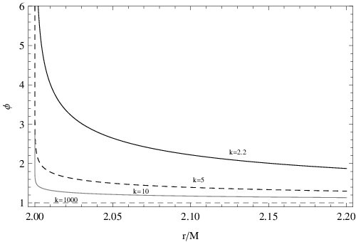
Moreover, as $r$ approaches $2M$ , $g_{tt}$ reduces to zero while $g_{55}$ explodes to infinity, therefore the length of the extra dimension increases as well as $r$ approaches $2M$ . It is possible to see that, at decreasing values of $k$ , at fixed $r/M$ the 5D-scale factor $\phi$ increases⁵⁵ 5 However as $r\to 2\left(1+10^{-6}\right)$ , for example, $\phi(k=2.2)=37.3618$ ., Fig. (1).

Refer to caption — Figure 1: The extra-dimensional scale factor $\phi=\sqrt{-g_{55}}$ as function of $r/M$ , for different values of $k$ .

Metric shows a pathological behavior as $r=2M$ . To investigate the nature of such a pathology we consider the values of one of the curvature invariants in that point. First we consider what happens in the five dimensional spacetime. The Kretschmann scalar $\ {}^{\mbox{\tiny{(5)}}}\!K_{1}\equiv R_{\mbox{\tiny{ABCD}}}R^{\mbox{\tiny{ABCD}}}$ is

\ {}^{\mbox{\tiny{(5)}}}\!K_{1}=\frac{48M^{4}}{r^{8}}\left(1-\frac{2M}{r}\right)^{2\epsilon(k-1)-4}

\left[\frac{r}{M}-1+\frac{\epsilon\left(\epsilon^{2}+1-2k+\sqrt{\epsilon^{4}-2k\epsilon^{2}-1}\right)}{2}\right]

\left[\frac{r}{M}-1+\frac{\epsilon\left(\epsilon^{2}+1-2k-\sqrt{\epsilon^{4}-2k\epsilon^{2}-1}\right)}{2}\right].

This quantity diverges as $r\rightarrow 2M$ . This fact suggests $r=2M$ as “real” singularity for the $\ {}^{\mbox{\tiny{(5)}}}\!M$ endowed with metric (24). The Kretschmann invariant $K_{1}$ of the Schwarzschild spacetime is recovered

K_{1}=\frac{48M^{2}}{r^{6}},

as one takes the limit $k\rightarrow\infty$ . Nevertheless to explore the solution behavior for radius close to $r=2M$ in the corresponding $\ {}^{\mbox{\tiny{(4)}}}\!M$ , we calculated the Kretschmann scalar $\ {}^{\mbox{\tiny{(4)}}}\!K_{1}=R_{abcd}R^{abcd}$ relative to the ordinary four dimensional spacetime

\ {}^{\mbox{\tiny{(4)}}}\!K_{1}=-\frac{24M^{4}}{r^{8}}\left(1-\frac{2M}{r}\right)^{2\epsilon(k-1)-4}\left(\epsilon^{2}-2\right)

\left(\frac{r}{M}-\frac{\epsilon\left[3+3\epsilon+2k\left(\epsilon^{2}-3\right)\right]-6}{3\left(\epsilon^{2}-2\right)}\right.

\left.\frac{-\epsilon\sqrt{(2+k)\epsilon^{4}+(1-6k)\epsilon^{2}-3}}{3\left(\epsilon^{2}-2\right)}\right)

\left(\frac{r}{M}-\frac{\epsilon\left[3+3\epsilon+2k\left(\epsilon^{2}-3\right)\right]-6}{3\left(\epsilon^{2}-2\right)}\right.

\left.\frac{+\epsilon\sqrt{(2+k)\epsilon^{4}+(1-6k)\epsilon^{2}-3}}{3\left(\epsilon^{2}-2\right)}\right).

This quantity diverges for $r\rightarrow 2M$ for any fixed values of $k>0$ . To evaluate the balance between the two limits, one for large values of k–parameter and the other for r close to the Schwarzschild horizon we also made the series of $\ {}^{\mbox{\tiny{(4)}}}\!K_{1}$ for $k\rightarrow\infty$ at some fixed value of $r$ , the first three terms are

\ {}^{\mbox{\tiny{(4)}}}\!K_{1}=\frac{48M^{2}}{r^{6}}-\frac{48M^{2}\ln\left[1-\frac{2M}{r}\right]}{kr^{6}}-\frac{4M^{2}(r-3M)\left(6r-11M\right)}{k^{2}r^{6}(r-2M)^{2}}+

+\frac{12M^{2}\ln\left[1-\frac{2M}{r}\right]\left(2\ln\left[1-\frac{2M}{r}\right]-5\right)}{k^{2}r^{6}}+O\left[\frac{1}{k}\right]^{3}

The Kretschmann invariant $K_{1}$ of the Schwarzschild spacetime is recovered as one takes the limit $k\rightarrow\infty$ . The other invariant we analyzed is the square of the Ricci tensor for the effective 4D–spacetime $\ {}^{\mbox{\tiny{(4)}}}\!K_{2}\equiv R_{ab}R^{ab}$

\ {}^{\mbox{\tiny{(4)}}}\!K_{2}=-\left(1-\frac{2M}{r}\right)^{2\epsilon(k-1)}\frac{2M^{4}\epsilon^{2}}{r^{4}(r-2M)^{4}}\left\{2Mr[3+\epsilon(2k-3)]\right.

\left.-3r^{2}+M^{2}\{\epsilon[6+2k(\epsilon-2)-\epsilon]-5\}\right\}

(25)

this quantity reduces in the Schwarzschild limit $\ {}^{\mbox{\tiny{(4)}}}\!K_{2}=0$ , for $k\rightarrow\infty$ at some fixed value of $r$ , the first non vanishing term is

\ {}^{\mbox{\tiny{(4)}}}\!K_{2}=\frac{2M^{2}\left(9M^{2}-10Mr+3r^{2}\right)}{r^{6}(-2M+r)^{2}k^{2}}+O\left[\frac{1}{k}\right]^{3}.

(26)

We have to conclude that the point $r=2M$ is a physical singularity in the 5D–manifold as for the ordinary 4D spacetime for all $k>0$ .

The GSS naked singularity is surrounded by the induced scalar matter with a trace free energy momentum tensor. The gravitational mass $M_{g}$ defined as ⁶⁶ 6 $dV_{3}$ is the ordinary spatial 3D–volume element

M_{g}=\int(T^{0}_{0}-T^{1}_{1}-T^{2}_{2}-T^{3}_{3})\sqrt{-g_{4}}dV_{3}

(27)

is, in the Schwarzschild limit, $M_{g}=M$ ; while, for each finite value of $k$ , it is $M_{g}=\epsilon kM$ at infinity and it goes to zero as $r$ closes the singularity.

4.1 Particle motion

The following conserved quantities characterize test particle motion in a GSS spacetime: $\mathcal{E}_{\mbox{\tiny{$\epsilon k$}}}\equiv\xi^{a}_{(t)}P_{a}$ , $L_{\mbox{\tiny{$\epsilon k$}}}\equiv\xi^{a}_{(\varphi)}P_{a}$ , where $\xi^{a}_{(t)}$ and $\xi^{a}_{(\varphi)}$ are metric Killing fields, or also

\displaystyle\mathcal{E}_{\epsilon k}\equiv\mathcal{E}\Delta^{k\epsilon-1},\;L_{\epsilon k}\equiv L\Delta^{(1-k)\epsilon+1}\,,

(28)

where $\mathcal{E}_{\mbox{\tiny{$\epsilon k$}}}=\mathcal{E}$ and $\mathcal{L}_{\mbox{\tiny{$\epsilon k$}}}=\mathcal{L}$ in the Schwarzschild’s limit where

\frac{E}{m}=\frac{(r-2M)}{\sqrt{r(r-3M)}};\quad\frac{L}{m}=\sqrt{\frac{r^{2}M}{(r-3M)}},

(29)

we interpret $\mathcal{E}_{\mbox{\tiny{$\epsilon k$}}}$ and $\mathcal{L}_{\mbox{\tiny{$\epsilon k$}}}$ as energy at infinity of the particle and total angular momentum, respectively. In terms of these quantities the lagrangian density $\mathcal{L}_{\mbox{\tiny{$\epsilon k$}}}$ is defined as follows:

\mathcal{L}_{\mbox{\tiny{$\epsilon k$}}}\equiv-m^{2}\Delta^{-\epsilon(k-1)}\left(\dot{r}\right)^{2}+\mathcal{E}_{\mbox{\tiny{$\epsilon k$}}}^{2}\Delta^{-\epsilon k}-L_{\mbox{\tiny{$\epsilon k$}}}^{2}r^{-2}\Delta^{\epsilon(k-1)-1}

(30)

Here $\dot{r}\equiv u^{r}$ , (see also[12] and [13, 14].

4.1.1 Equatorial orbits

The effective potential $V_{\mbox{\tiny{$\epsilon k$}}}\equiv E/m$ , for massive test particles in an equatorial orbit (with $k\geq 1$ ) is defined as follows:

V_{\mbox{\tiny{$\epsilon k$}}}\equiv\sqrt{g_{\mbox{\tiny{00}}}\left(1-\frac{L_{\mbox{\tiny{$\epsilon k$}}}^{2}}{m^{2}g_{\varphi\varphi}}\right)}\,.

(31)

Studying $V_{\mbox{\tiny{$\epsilon k$}}}$ as function of the orbit radius $r$ , we find the particle energy $\mathcal{E}_{\mbox{\tiny{$\epsilon k$}}}$ and the angular momentum $L_{\mbox{\tiny{$\epsilon k$}}}$ of circular orbits: they are

	$\displaystyle\frac{\mathcal{E}_{\mbox{\tiny{$\epsilon k$}}}}{m}$	$\displaystyle=$	$\displaystyle\Delta^{\frac{k\epsilon}{2}}\sqrt{1+\frac{\epsilon k}{\epsilon(1-2k)+\left(\frac{r}{M}-1\right)}},$		(32)
	$\displaystyle\frac{L^{\pm}_{\mbox{\tiny{$\epsilon k$}}}}{mM}$	$\displaystyle=$	$\displaystyle\pm\sqrt{\frac{\epsilon k\frac{r^{2}}{M^{2}}\Delta^{\left[(1-k)\epsilon+1\right]}}{\epsilon\left(1-2k\right)+\left(\frac{r}{M}-1\right)}}.$		(33)

[12]. Last circular orbit radius is

\displaystyle r_{lco}=\left[1+\epsilon(2k-1)\right]M\,,

(34)

where $r_{lco}<3M$ and approaches this limit when $k$ goes to infinity [12, 18]. On the other side, as $k$ approaches smaller values, last circular orbits radius approaches the point $r=2M$ Fig. (2); for $k=1$ it is $r_{lco}\equiv 2M$ . This fact suggests to check for circular orbits situated in a region avoided by the 4D–Schwarzchild’s physics. The aim of the next part of this section is to explore the stability of such orbits. First, effective potential has two turning points located in $r^{\pm}/M=\left[1+\epsilon(3k-2)\pm\epsilon\sqrt{(k-1)(4k-1)}\right]M$

where in the Schwarzschild’s limit $r^{+}\equiv 6M$ ad $r^{-}\equiv 2M$ . We infer also from this fact that last stable circular orbit radius is

r_{lsco}=\left[1+\epsilon(3k-2)+\epsilon\sqrt{(k-1)(4k-1)}\right]M\,.

(35)

While in the Schwarzschild’s limit we have $r_{lsco}\equiv 6M$ , here it is $r_{lsco}<6M$ $\forall k>1$ and for $k=1$ we have $r_{lsco}=2M$ ; this remarkably aspect of the circular motion in the GSS spacetime could be a valid constraint to the theory implying particles in stable orbits for values of radius just less than $6M$ .

Finally, another orbital deformation induced by the compactified fifth dimension appears in the values of the energy and angular momentum of the last stable circular orbits: the energy $\mathcal{E}_{lsco}=\mathcal{E}_{\mbox{\tiny{$\epsilon k$}}}(r_{lsco})$ is always below its Schwarzschild’s limit ( $E_{lsco}=\frac{2\sqrt{2}}{3}m=0.942809m$ ) for all values of $k\gtrsim 1$ , while the angular momentum $\mathcal{L}_{lsco}=\mathcal{L}_{\epsilon k}(r_{lsco})$ is over the Schwarzschild’s limit ( $L_{lsco}=2\sqrt{3}Mm=3.4641Mm$ ) value for $k>3.45644$ , Fig. (3).

4.1.2 Radially falling particles

We consider here vertical free falling test particles in the GSS-background. To begin with, we note at first that the motion will be described by $\dot{\theta}=\dot{\phi}=0$ . Particle motion will be regulated by the $t$ -component and $r$ -component of the geodesic equation (11). However, radial motion has been extensively studied in literature, see for example [9, 43]. We review here the main results and point out some considerations based on the interpretation given by the Papapetrou’s approach. Particular attention is devoted to the dynamics in a region close to the singularity ring $r=2M$ .

From (30) we infer:

\Delta^{-\epsilon k}\mathcal{E}_{\mbox{\tiny{$\epsilon k$}}}^{2}-m^{2}\Delta^{-\epsilon(k-1)}\left(\dot{r}\right)^{2}\equiv 1\,.

(36)

[9]. The coordinate velocity component in the $r$ -direction is $v_{r}\equiv r^{\prime}=dr/dt$ . For a particle starting from a point at (spatial) infinity we have:

\frac{dr}{dt}=-\Delta^{\epsilon k-\epsilon/2}\sqrt{1-\Delta^{\epsilon k}}\,.

(37)

The locally measured radially velocity is $v_{r_{*}}\equiv r^{\prime}_{*}=dr^{*}/dt$ where $dr/dr^{*}=\sqrt{g_{tt}/g_{rr}}=\Delta^{\epsilon k-\epsilon/2}$ . Therefore we can write

\frac{dr^{*}}{dt}=-\sqrt{1-\Delta^{\epsilon k}}\,,

(38)

where $v_{r}$ and $v_{r^{*}}$ are function of $(r,k)$ . Both converge to zero at (spatial)-infinity. The radial velocity $v_{r}$ goes to zero in the limit $r\rightarrow 2M$ , Fig. (4), and the local measured velocity $v_{r^{*}}$ goes to $(-1)$ in the limit $r\rightarrow 2M$ , Fig. (5).

The evaluation for $r^{*}$ is given as follows:

	$\displaystyle\frac{r^{*}}{M}=2\left(2-\frac{r}{M}\right)^{\frac{(2k-1)\epsilon}{2}}\left(\frac{r}{M}-2\right)^{\frac{(1-2k)\epsilon}{2}}$
	$\displaystyle B\left[\frac{r}{2M},1-\frac{\epsilon}{2}+\epsilon k,\frac{\epsilon(1-2k+\frac{2}{\epsilon})}{2}\right]+C[k]\,.$		(39)

We have the incomplete beta function $B[x,a,b]=B_{x}(a,b)$ where $C[k]$ is a (imaginary)-constant of integration, to be fixed in agreement to the Schwarzschild’s limit and the reality condition of the solution. However, $r^{*}$ always goes to infinity at (spatial)–infinity. The picture is much more complex close to the point $r=2M$ ; it strongly depends of the particular GSS solution, being $r^{*}(2M)$ a function of $k$ . Indeed, for a fixed value of $k$ , $r^{*}(2M)$ is a negative number that approaches to $(-\infty)$ as well as $k\rightarrow\infty$ Fig. (6).

In agreement with [43] , the radius $\varrho$ , at which the radial velocity $r^{\prime}$ starts to decreases, is

\varrho=2M\left[1-\left(\frac{2k-1}{3k-1}\right)^{1/(\epsilon k)}\right]^{-1}\,,

(40)

that in the Schwarzschild’s limit reduces to $\varrho=6M$ , otherwise we have $\rho=\rho(k)<6M$ Fig. (7).

5 The interior solution

The KK–equations (18–20) for the free electromagnetic case with $\vartheta=0$ are,

$\displaystyle G^{\mu\nu}$	$\displaystyle=$	$\displaystyle\frac{1}{\phi}\left(\nabla^{\mu}\partial^{\nu}\phi-g^{\mu\nu}\Box\phi+8\pi GT^{\mu\nu}_{\mbox{\tiny{matter}}}\right),$
		$\displaystyle\nabla_{\rho}\left(T^{\mu\rho}_{\mbox{\tiny{matter}}}\right)=0,\quad R=0,$
$\displaystyle\Box\phi$	$\displaystyle=$	$\displaystyle\frac{8\pi}{3}\left(T_{\mbox{\tiny{matter}}}\right).$	(41)

where $T_{\mbox{\tiny{matter}}}\equiv g_{\mu\nu}T^{\mu\nu}_{\mbox{\tiny{matter}}}$ . GSS is a solution of eqs. (41) with $T^{\mu\nu}_{\mbox{\tiny{matter}}}=0$ . We consider a (4D) perfect fluid energy momentum tensor, $T^{\mu\nu}_{\mbox{\tiny{matter}}}\equiv T^{\mu\nu}$ :

T_{\mu\nu}=(p+\rho)u_{\mu}u_{\nu}-pg_{\mu\nu}.

(42)

where $p$ is the pressure, $\rho$ the density. Therefore eqs. (41) became

	$\displaystyle G_{\mu\nu}$	$\displaystyle=$	$\displaystyle\frac{1}{\phi}\left(\nabla_{\mu}\partial_{\nu}\phi-g_{\mu\nu}\frac{8\pi}{3}\left(\rho-3p\right)+8\pi T_{\mu\nu}\right),$		(43)
	$\displaystyle\Box\phi$	$\displaystyle=$	$\displaystyle\frac{8\pi}{3}\left(\rho-3p\right),\quad\nabla_{\rho}\left(T^{\mu\rho}\right)=0.$		(44)

We look for a solution of eqs. (43, 44) that matches the GSS on a certain radius $r=R$ where $p(R)=0$ . In order to do this we considered an equation of state $p=a\rho^{b}$ with $(a,b)$ constants and a metric solution of the form⁷⁷ 7 Consider $t\in\Re$ , $r\in\left]0,+\infty\right]\subset\Re^{+}$ , $\vartheta\in\left[0,\pi\right]$ , $\varphi\in\left[0,2\pi\right]$

ds_{\mbox{\tiny{(5)}}}^{2}=fdt^{2}-hdr^{2}-qd\Omega^{2}-\phi^{2}(dx^{5})^{2},

(45)

where $(f,h,q,\phi)$ are functions of $r$ only. From the conservation equation in (44) we obtain

f(r)=c\left(\frac{\rho(r)}{\rho(r)+a\rho(r)^{b}}\right)^{\frac{2b}{b-1}},

(46)

where the constant $c$ must be fixed to match the exterior solution(GSS). Noting that the equations do not change under the transformation $f(r)\rightarrow f(r)/c$ , the solution (46) is substituted in the set eqs. (43, 44). We integrated numerically the three independent equations, the $(tt)$ $(rr)$ components of the Einstein equations and the Klein Gordon equation, for the variables $\Delta,\phi$ , and $\rho$ where

h(r)=\Delta(r)^{-\epsilon(k-1)},\quad q(r)=\Delta(r)^{1-\epsilon k-1)},

(47)

and $\Delta(r)$ is now an unknown function of the radial coordinate. To establish the initial conditions we imposed

	$\displaystyle\phi_{0}$	$\displaystyle\equiv$	$\displaystyle\phi(0)=\left(1-\frac{2}{x}\right)^{-\epsilon/2},$		(48)
	$\displaystyle\phi^{\prime}_{0}$	$\displaystyle\equiv$	$\displaystyle\phi^{\prime}(0)=-\frac{\epsilon\left(1-\frac{2}{x}\right)^{-(1+\frac{\epsilon}{2})}}{x^{2}}.$		(49)

Therefore, for fixed values of $a,b$ and $\rho_{0}$ , we solved an “eigenvalue” problem for $x$ , where $x$ is fixed to verify the match conditions

$\displaystyle\Delta(R)$	$\displaystyle=$	$\displaystyle\left(1-\frac{2}{R}\right),\quad\Delta^{\prime}(R)=\frac{2}{R^{2}},$	(50)
$\displaystyle\phi(R)$	$\displaystyle=$	$\displaystyle\left(1-\frac{2}{R}\right)^{-\epsilon/2},$	(51)
$\displaystyle\phi^{\prime}(R)$	$\displaystyle=$	$\displaystyle-\frac{\left(1-\frac{2}{R}\right)^{-1-\frac{\epsilon}{2}}\epsilon}{R^{2}}.$	(52)

Some solutions, for different values of $k$ , are plotted in Fig. (8).

The index $b$ has been fixed $b=4/3$ . Four different cases of $k\in\{2.2,5,10,1000\}$ have been considered. Thus, the Einstein-Klein-Gordon equations have been integrated for a fixed central density $\rho(0)$ . In the recovered solutions the interior ordinary 4D matter is characterized by a polytropic equation of state $p(\rho)=a\rho^{4/3}$ . The integration procedure leads to a constant $a\approx 0.4$ , for each values of $k$ and $\rho_{0}$ . The central density $\rho_{0}$ decreases increasing the $k$ parameter. In this configurations the scalar field matter, solution of massless Klein-Gordon equation is coupled to this matter by Eq. (44).

The physical proprieties of each solutions and the astrophysical implications of their existence requires a more detailed investigation and it will be discussed elsewhere [19].

6 Furthers applications

We conclude this discussion briefly introducing the possible concrete applications of the analysis of the interior, stellar solutions associated to the GSS family of metrics.

Stellar models in extended or higher dimensional theories of gravity have been extensively studied in literature, in many contexts (see for example [20, 21, 22, 23, 24, 25, 26, 27, 28]).

For example, it could be interesting to compare with other alternative proposals where stellar solutions are derived. In view of this, we consider, for instance, the results reported in [20] in which the hydrostatic equilibrium and stellar structure in $f(R)$ gravity has been studied. As well enlighted in [20] the strong gravity regime is a valuable way to check the validity of the extended and the multidimensional theories of gravity, in particular the formation and the evolution of stars can be considered suitable test for these theories.

The study of stars in five dimensional Kaluza Klein gravity could develop in two main directions that are also future developments on this work: the extensive study of the phenomena around the 4D stellar objects and the comprehension of the dynamics of such kind of objects.

In the compactification hypothesis is predominant the idea to find a possible field of phenomena in which the presence of the extra dimension takes evidence. This fact has to be taken seriously into account especially in those contexts in which the strong gravity effects could matches the physics of the Planck scale [29]. On one side, attention is for example devoted to the microphysics of the LHC to search for a sign of the Planck scale length dimension [30, 31, 32, 33], but many efforts are also given to the comprehension of the higher energy astrophysical phenomena linked to the life steps of stellar evolution and that could be a natural arena in which explore the effects of a multidimensional theory [34, 35], especially for those cases in which the standard models of stellar structure and evolutions does not properly collide with observed data; suggesting therefore a different or a modification of the basic mechanics that rules stars matter and life [36]). An example can be provided by the magnetars or anomalous neutron stars, (see for example [20] and reference therein).

The exploration of the motions in the vacuum spacetime, partially faced here and in [12, 38] within the Papapetrou approach can be completed by the analysis of the emission processes induced by charged particles in the GSS background. The comparison in particular of the electromagnetic emission spectra due to a freely falling charged test particle, and in general the test particle dynamics, in the GSS and in Schwarzschild background could get light on physics around the singular ring $r=2M$ , whose naked singularity nature is actually ambiguous (see also [39, 40] and [41, 42]). However the solution of the equations governing the emission process should strongly depend on the boundary conditions imposed on the equations. A comparison between the electromagnetic emission by radially falling charged particles in the GSS and stellar case could be strongly discriminant.

7 Conclusions

The aim of this work was to verify the existence of an interior solution of the KK–equations to mach with the vacuum spacetime of the Generalized Schwarzschild solution characterized by a naked singularity. For this purpose we solved the set of five dimensional static, electromagnetic-free KK–equations. These have been numerically integrated for a (4D) perfect fluid energy momentum tensor with a polytropic equation of state. These solutions are matched with the Generalized Schwarzschild solution.

There is a great interest in providing a theoretical model able to explain the role of the extra dimensions and their compatibility in a world that looks like a four dimensional one.

Therefore any experimental observation compatible with such theories could be a strong constraint concerning their validity for example by exploring the dynamical effects of the extra compactified dimension. Using an effective potential approach to the motion, we showed the last circular orbit radius and in particular the last stable circular orbits radius of a charged or neutral test particles [12]. The detailed study of the physical features on such astrophysical objects will be a future work.

The study of bounded configurations in KK–paradigm is intriguing for many respects: from one side it could represent an environment in which an hypothetical extra dimension shows a recognizable fingerprint on the dynamics and global properties of these objects. On the other side the interior solutions for the GSS–like spacetime are particular interesting if the GSS is read as KK–generalization of a Schwarzschild metric for an electrically neutral spherically symmetric 4D–object. In fact, if the final state of the star evolution in the Schwarzschild spacetime could lead to a 4D–black hole, the final state of an neutral spherically symmetric 4D–object in GSS should lead to a naked singularity for the ordinary 4D–spacetime. Nevertheless both the solutions describe neutral spherically symmetric 4D–object the difference being in the presence, for the KK–solution, of a coupling with a scalar matter. In this respect, the comprehension of the mechanisms under these different evolutions of the neutral spherically symmetric 4D–object, one in the general relativistic framework, and the other with the contribution of a scalar field in the GSS, is challenging, [47, 46, 45, 44].

Acknowledgments

This work has been developed in the framework of the CGW Collaboration (www.cgwcollaboration.it). We would like to thank V. Lacquaniti for helpful comments on this topic. One of us (DP) gratefully acknowledges financial support from the A. Della Riccia Foundation.

References

(1) T. Kaluza, On the Unity Problem of Physics, Sitzungseber. Press. Akad. Wiss. Phys. Math. ,1921.
(2) O. Klein, Z.F.Physik, 37, 1926.
(3) O. Klein, Nature, 118, 1926.
(4) D. Bailin and A. Love, Rept. Prog. Phys. 50 (1987) 1087.
(5) Modern Kaluza-Klein Theories, edited by T. Applequist, A. Chodos, and P.G.O. Freund, Addison-Welsey, Menlo Park, 1987.
(6) J. Polchinski, String Theory Vol. 1, Cambridge University Press (1998).
(7) J. Clifford, D-branes, Cambridge University Press (2003)
(8) J. Wess and J. Bagger, Supersymmetry and Supergravity. Princeton Univ. Press, Princeton, NJ, 1992.
(9) J. M. Overduin and P. S. Wesson, Phys. Rept. 283 (1997) 303.
(10) F. Cianfrani and G. Montani, arXiv:0904.0574 [gr-qc].
(11) P. S. Wesson, Space-time-matter: Modern Kaluza-Klein theory, Singapore, Singapore: World Scientific (1999).
(12) V. Lacquaniti, G. Montani, D. Pugliese, Gen. Rel. Grav. DOI:10.1007/s10714-010-1007-3.
(13) E. Hackmann, V. Kagramanova, J. Kunz and C. Lammerzahl, Phys. Rev. D 78 (2008) 124018 [Erratum-ibid. 79 (2009) 029901].
(14) V. Z. Enolski, E. Hackmann, V. Kagramanova, J. Kunz and C. Lammerzahl, J. Geom. Phys. 61, 899 (2011).
(15) J. Ponce de Leon Int.J.Mod.Phys.D18:251-273,2009.
(16) V. Lacquaniti and G. Montani, arXiv:0906.2231.
(17) V. Lacquaniti and G. Montani, Mod. Phys. Lett. A 24 (2009) 1565.
(18) V. Lacquaniti and G. Montani, Int. J. Mod. Phys. D 18 (2009) 929.
(19) G. Montani, D. Pugliese, in preparation.
(20) S. Capozziello, M. De Laurentis, S. D. Odintsov and A. Stabile, Phys. Rev. D 83 (2011) 064004.
(21) N. Kan and K. Shiraishi Phys. Rev. D 66, 105014 (2002).
(22) J. Ponce de Leon, Grav. Cosmol. 14 (2008) 65.
(23) J. P. de Leon, Class. Quant. Grav. 24 (2007) 1755.
(24) L. K. Patel and G. P. Singh, Grav. Cosmol. 7, 52 (2001).
(25) P. K. Chattopadhyay, B. C. Paul, PRAMANA, journal physics, Vol. 74, No. 4, 2010 pp. 513-523.
(26) B. C. Paul, Int. J. Mod. Phys. D, Vol. 13, Issue 02, pp. 229-238 (2004).
(27) U. Bleyer, L.S. Grigorian, H.F. Khachatrian Astrophysics, Vol. 39, No. 4, 359-369.
(28) U. Bleyer, L.S. Grigorian, Astrophysics and Space Science, vol. 225, no. 1, p. 123-135.
(29) S. Capozziello, G. Cristofano and M. De Laurentis, Eur. Phys. J. C 69 (2010) 293.
(30) K. Kong, K. Matchev and G. Servant, arXiv:1001.4801 [hep-ph].
(31) B. Bhattacherjee and K. Ghosh, Phys. Rev. D 83 (2011) 034003.
(32) A. Datta, K. Kong and K. T. Matchev, New J. Phys. 12 (2010) 075017.
(33) R. Franceschini, G. F. Giudice, P. P. Giardino, P. Lodone and A. Strumia, arXiv:1101.4919 [hep-ph].
(34) G. G. Barnafoldi, P. Levai and B. Lukacs, J. Phys.: Conf. Ser. 218 012010 doi: 10.1088/1742-6596/218/1/012010.
(35) G.G. Barnafoldi, P. Levai, B. Lukacs, Astronomische Nachrichten, Volume 328, Issue 8, pages 809812, October 2007 .
(36) S. Hannestad and G. G. Raffelt, Phys. Rev. D 67 (2003) 125008 [Erratum-ibid. D 69 (2004) 029901].
(37) A. Papapetrou, Proc. Phys. Soc. 64, 57 (1951).
(38) V. Lacquaniti, G. Montani, D. Pugliese, arXiv:0911.4168 [gr-qc].
(39) K. S. Virbhadra and C. R. Keeton, Phys. Rev. D 77 (2008) 124014.
(40) K. S. Virbhadra and G. F. R. Ellis, Phys. Rev. D 65 (2002) 103004.
(41) H. Liu and P. S. Wesson, J. Math. Phys. 42, 4963 (2001).
(42) M. Cassé, J. Paul, G. Bertone, G. Sigl Phys. Rev. Lett. 2004 Mar 19;92(11):111102.
(43) D. Kalligas, P. S. Wesson and C. W. F. Everitt, Astrophys. J. 439 (1994) 548.
(44) M. Eingorn and A. Zhuk, Phys. Rev. D 83 (2011) 044005.
(45) M. Eingorn, O. R. de Medeiros, L. C. B. Crispino and A. Zhuk, arXiv:1101.3910 [gr-qc].
(46) J. P. de Leon, arXiv:1003.3151 [gr-qc].
(47) Y. Yamada and H. a. Shinkai, arXiv:1102.2090 [gr-qc].