Constructions of hamiltonian graphs with bounded degree and diameter Thanks: Supported by the Research Program P1-0285 of Slovenian Agency for Research and the Grant 144007 of Serbian Ministry of Science and Technological Development.
Abstract
Token ring topology has been frequently used in the design of distributed loop computer networks and one measure of its performance is the diameter. We propose an algorithm for constructing hamiltonian graphs with vertices and maximum degree and diameter , where is an arbitrary number. The number of edges is asymptotically bounded by . In particular, we construct a family of hamiltonian graphs with diameter at most , maximum degree and at most edges.
Keywords: hamiltonian cycle, token ring, diameter, binary tree, graph algorithm
1 Introduction
An undirected graph can be used as a mathematical model for computer networks, where is the set of vertices and is the set of edges. The number of edges adjacent to a vertex is called the degree of the vertex . A graph is regular if all vertices have equal degrees. The distance between two vertices and is the number of edges on a shortest path between and . The diameter of the graph is the maximum distance between any pair of vertices: . A cycle is a sequence of three or more vertices such that two consecutive vertices are adjacent and with no repeated vertices other than the start and end vertex. A hamiltonian cycle is a cycle that visits each vertex of a graph exactly once. A graph is -hamiltonian if, after removing an arbitrary vertex or an edge, it still remains hamiltonian. A -hamiltonian graph G is optimal if it contains the least number of edges among all -hamiltonian graphs with the same number of vertices as .
Networks with at least one ring structure (hamiltonian cycle) are called loop networks. Distributed loop networks are extensions of ring networks and are widely used in the design and implementation of local area networks and parallel processing architectures. There are many mutually conflicting requirements when designing the topology of a computer network. For example, no pair of processors should be too far apart in order to support efficient parallel computation demands. The hamiltonian property is one of the major requirements. The token passing is a channel access method where data is transmitted sequentially from one ring station to the next with a control token circulating around the ring controlling access.
An open problem considered in a survey [2] on distributed loop networks is following: Find hamiltonian networks, -regular on vertices with a diameter of order . This problem is related to the famous problem in which we want to construct a graph of vertices with maximum degree such that the diameter is minimized, but hamiltonicity is not an issue. The lower bound on the diameter is called the Moore bound,
Harary and Hayes [6] presented a family of optimal -hamiltonian planar graphs on vertices. Wang, Hung and Hsu [12] presented another family of optimal -hamiltonian graphs, each of which is planar, hamiltonian, cubic, and of diameter . In the literature three other families of cubic, planar and optimal -hamiltonian graphs with diameter are described. These constructions are possible only for special choices of , as shown in Table 1.
| Reference | Name | Comment | ||
|---|---|---|---|---|
| Wang et al. [11] | Eye graph | -connected | ||
| Hung et al. [7] | Christmas tree | hamiltonian connected | ||
| Kao et al. [8] | Brother tree | bipartite |
The best constructions for cubic graphs have diameter (see [4]). It is shown in [3] that a cubic graph obtained by adding a random perfect matching to a cycle has a diameter of order . In the same paper, the authors proved the following result:
Theorem 1.1
Suppose is a complete binary tree on vertices. If we add two random matchings of size to the leaves of , then the resulting graph has diameter satisfying
with probability approaching as approaches infinity.
In [10] it is shown that almost all -regular graphs are hamiltonian for any , by an analysis of the distribution of -factors in random regular graphs.
In this paper we propose an algorithm for constructing hamiltonian graphs with vertices, maximum degree and diameter bounded by:
Our main contribution is that we assure diameter for every , not just for special values, while hamiltonicity and small diameter are achieved by using significantly less edges.
The paper is organized as follows. In Section 2 we describe the linear algorithm and prove that it produces hamiltonian graphs of degree at most and diameter at most . In Section 3 we deal with the case and improve the upper bound for the number of edges in the resulting graph to . The same approach may be applied for and this way we get a hamiltonian graph with the average degree asymptotically equal to . In the end, we show that the algorithm may be modified in such a way that it constructs a planar hamiltonian graph with degree at most and diameter at most and also point out some experimental results for diameter when .
2 The algorithm
A complete binary tree is a tree with levels, where for each level , the number of the existing nodes at level equals . This means that all possible nodes exist at these levels. An additional requirement for a complete binary tree is that for the -th level, while not all nodes have to exist, the nodes that do exist must fill the level from left to right (for more details see [5]). A complete binary tree is one of the most important architectures for interconnection networks [9].
A generalization of binary trees are -ary trees. Namely, every vertex has at most children, and all vertices that are not in the last level have exactly children. All vertices in the last level must occupy the leftmost spots consecutively.
We propose the following algorithm for constructing hamiltonian graphs of order , maximum degree and diameter . First we construct a complete -ary tree with vertices, and for every vertex we store its degree, parent, and all children from left to right. A labeled -ary tree contains labels through with root being , branches leading to nodes labeled , branches from these leading to , and so on. We also maintain a queue of all leaves.
We will traverse vertices in order to form a hamiltonian cycle. The starting vertex is the root of the tree. First we try to go up the tree through the parent of the current vertex - if the parent is already visited, we choose one of its children. In the case where all neighbors of the current vertex are marked, we pick an arbitrary unmarked leaf and add an edge connecting these two vertices.
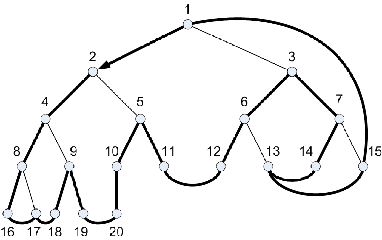
Theorem 2.1
A graph constructed by the above algorithm is hamiltonian.
Proof: The basic idea of the algorithm is to traverse the hamiltonian path by adding edges when they are needed. In the end, we join the last visited vertex to the root of the binary tree. There can be at most one vertex other than the root with a degree greater than and less than in the tree - let this vertex have the label . All edges that we add during the execution of the algorithm connect either two leaves or a leaf and . By symmetry, we can eliminate the vertex by traversing from the root to in the first few steps of the algorithm. Therefore, this algorithm does not increase the maximum degree in the graph.
We cannot visit any vertex twice, so we have to prove that all vertices are marked. Assume that the vertex is not visited and the algorithm has finished. If any vertex in its subtree is visited, then we would have already visited , because we first try to go upwards. Therefore, all vertices in its subtree are unvisited. There is at least one leaf in the subtree, and we have to visit this leaf during the execution of the algorithm. This is a contradiction, so the constructed graph is hamiltonian.
The diameter of this graph is less than or equal to twice the depth of the tree.
Lemma 2.1
The number of leaves in a complete -ary tree is
Proof: We know that and for . Whenever we properly add vertices to this tree, we always get exactly new leaves. This proves the recurrent relation for the number of leaves
By mathematical induction, one can easily prove the explicit formula for .
Theorem 2.2
The number of edges in the constructed graph is less than .
Proof: There are edges in a -regular graph. The internal nodes in a -ary tree are nodes with degree greater than one. After running the algorithm, every leaf will have degree at most three and every internal node will have degree at most . This gives an upper bound for the number of edges in the hamiltonian graph constructed by the algorithm:
This bound is less than for , and less than if and the depth of the tree is greater than two. Based on this fact, we give the following
Proposition 2.1
Time and memory complexity of the proposed algorithm is linear .
3 Number of edges added for
Cubic graphs are of special interest in token ring topologies and because of their importance, in this section we improve the previous estimations for the number of edges added in the construction of a hamiltonian path for the case .
First we examine graphs with vertices, where . A corresponding binary tree has complete last level and there are leaves in the tree. Let be the number of additional edges added to this tree, when we start the execution of the algorithm in an arbitrary leaf and end it in another leaf. One can easily verify that and . In addition, we define . After traversing upwards to the root and then downwards to an arbitrary leaf, the graph induced by the unvisited vertices are disjoint complete binary trees of heights . Therefore, we may write the recurrent formula:
By strong induction we will prove that:
Assume that the formula holds for all numbers , and now we will prove it for and .
To estimate the actual number of additional edges in the proposed algorithm we have to start from the root and add an additional edge connecting the last visited vertex and the root of the binary tree. After visiting the first leaf we have that the unvisited vertices form disjoint complete binary trees of heights and . So, the total number of edges to be added equals:
Therefore, we proved the following result.
Theorem 3.1
The number of additional edges in the case of a complete binary tree with vertices does not depend on the choice of random leaves in the algorithm and this number equals .
Now assume that is not of the form . The main result in this section is the following theorem.
Theorem 3.2
For every integer , there exists a hamiltonian graph with diameter at most , maximum degree and at most edges.
Proof: The number of leaves in a corresponding binary tree with vertices is . Some leaves are on the last level, and some are on the level before last. Consider the consecutive leaves in the last level starting from the left and group them into groups of size four. This way we get subtrees of height two and there can be at most three unpaired leaves. We will do the same thing for the leaves in the previous level, but starting from the right.
Therefore, the number of subtrees of height two is less than or equal to and greater than . According to the two cases in Figure 2, there can be two or three leaves in each of these subtrees that will get and keep degree two until the algorithm finishes. Thus, the number of edges we do not have to add equals half the number of vertices of degree two, and it is between and . The total number of edges in the constructed graph after running the algorithm will be between and .

Remark 3.1
After the hamiltonian cycle is constructed, we may insert additional edges into the graph to make it cubic, provided is even.
For the case , one can construct a hamiltonian graph with at most
edges. The same approach may be applied to complete binary subtrees of greater heights to obtain a slightly finer bound for the total number of edges.
4 Concluding remarks
The proposed algorithm may be modified to construct a planar hamiltonian graph.
Theorem 4.1
By appropriately choosing descendant and unvisited leaves in the algorithm, one can assure that the constructed graph is planar.
Proof: In order to prove the theorem, we will construct a hamiltonian path that starts at the leftmost leaf and ends in the nearest leaf (neighboring leaf or leaf that is at distance three from it). For small values of , this can be easily verified. In the general case we first go upwards to the root and then to the rightmost leaf. Now, the -ary tree is partitioned into smaller trees, which will be traversed by induction from left to right. These binary trees do not have vertices in common, and we can independently add necessary edges which do not intersect the existing edges. We reduce our problem to the previous case by going to the leftmost leaf. Now we have disjoint trees and we traverse them starting from the leaves. Finally, we add the last edge without intersection problems (as in Figure 1).
For the case , in our implementation we always choose a leaf that is farthest from the current leaf. This heuristic is done by the breadth first search. We use only three arrays of length , so memory requirements are linear in . Time complexity is , because the number of edges is . The diameters of the examples of cubic graphs constructed by this algorithm are shown in Figure 3, where the -axis carries and is the number of nodes. It is obvious from this figure that the constant from our bound is not the best possible.

Instead of choosing the leaves at random, we can do it more sophisticatedly and further reduce the diameter of the graph. One possible way is to add a matching which connects only the leaves on the last level in the root’s left and right subtree. This way we can still apply the algorithm, but if we have to choose a random leaf to continue—we first check whether the paired leaf in the matching is marked. This way we decrease the diameter by a constant, which is at least one. We leave for future study to see whether this approach may be used to construct -edge hamiltonian graphs.
Acknowledgement: The authors are grateful to the reviewers for their valuable comments and suggestions.
References
- [1] N. Alon, A. Gyárfás, M. Ruszinkó: Decreasing the diameter of bounded degree graphs, Journal of Graph Theory 35 (2000), 161–172
- [2] J. C. Bermond, F. Comellas, D. F. Hsu: Distributed Loop Computer Networks: A Survey, Journal of Parallel and Distributed Computing 24 (1995), 2–10
- [3] B. Bollobás, F. R. K. Chung: The diameter of a cycle plus a random matching, SIAM Journal on Discrete Mathematics 1 (1988), 328–333
- [4] M. Capalbo: An explicit construction of lower diameter cubic graphs, SIAM Journal on Discrete Mathematics 16 (2003), 630–634
- [5] T. H. Cormen, C. E. Leiserson, R.L. Rivest, C. Stein: Introduction to Algorithms, Second Edition, MIT Press, 2001.
- [6] F. Harary, J. P. Hayes: Node fault tolerance in graphs, Networks 27 (1996), 19–23
- [7] Chun-Nan Hung, Lih-Hsing Hsu, Ting-Yi Sung: Christmas tree: A versatile 1-fault-tolerant design for token rings, Information Processing Letters 72 (1999), 55–63
- [8] Shin-Shin Kao, Lih-Hsing Hsu: Brother trees: A family of optimal -hamiltonian and -egde hamiltonian graphs, Information Processing Letters 86 (2003), 263–269
- [9] F. T. Leighton: Introduction to Parallel Algorithms and Architectures: Arrays, Trees and Hypercubes, Morgan Kaufmann, San Mateo, CA, 1992.
- [10] R. W. Robinson, N. C. Wormald: Almost all regular graphs are hamiltonian, Random Structures and Algorithm, Volume 5 (2), (1992), 363–374
- [11] Jeng-Jung Wang, Ting-Yi Sung, Lih-Hsing Hsu, Men-Yang Lin: A New Family of Optimal 1-hamiltonian Graphs with Small Diameter, Proceedings of the 4th Annual International Conference on Computing and Combinatorics (1998), 269–278
- [12] Jeng-Jung Wang, C.N. Hung, L. H. Hsu: Optimal -hamiltonian graphs, Information Processing Letters 65 (1998), 157–161