A natural little hierarchy for RS
from accidental SUSY
Tony Gherghetta11 1 E-mail: tgher@unimelb.edu.au,a,b, Benedict von Harling22 2 E-mail: bvo@unimelb.edu.au,a and Nicholas Setzer33 3 E-mail: nsetzer@unimelb.edu.au,a
aSchool of Physics, University of Melbourne, Victoria 3010,
Australia
bStanford Institute of Theoretical Physics, Stanford University, Stanford, CA 94305,
USA
Abstract
We use supersymmetry to address the little hierarchy problem in Randall-Sundrum models by naturally generating a hierarchy between the IR scale and the electroweak scale. Supersymmetry is broken on the UV brane which triggers the stabilization of the warped extra dimension at an IR scale of order 10 TeV. The Higgs and top quark live near the IR brane whereas light fermion generations are localized towards the UV brane. Supersymmetry breaking causes the first two sparticle generations to decouple, thereby avoiding the supersymmetric flavour and problems, while an accidental -symmetry protects the gaugino mass. The resulting low-energy sparticle spectrum consists of stops, gauginos and Higgsinos which are sufficient to stabilize the little hierarchy between the IR scale and the electroweak scale. Finally, the supersymmetric little hierarchy problem is ameliorated by introducing a singlet Higgs field on the IR brane.
1 Introduction
A warped extra dimension provides a natural way to explain hierarchies in the standard model. In the five-dimensional () warped geometry the local cutoff is position dependent. By localizing the Higgs sector on the infrared (IR) brane, the Higgs cutoff can be naturally of order the TeV scale, thereby providing a solution to the gauge hierarchy problem [1]. Furthermore by placing the standard model fermions in the bulk, large hierarchies in the Yukawa couplings can be explained by a wavefunction overlap with the Higgs boson in the extra dimension [2, 3, 4]. This fermion and Higgs geography in the slice of AdS5 therefore provides a novel framework to address hierarchies in the standard model without symmetries or hierarchies in the Yukawa couplings (often referred to as anarchic couplings).
However, with anarchic couplings, -violating processes mediated by Kaluza-Klein (KK) modes are in excess of experimental bounds unless the IR scale is at least [5, 6, 7]. Although this bound can be avoided with additional structure (such as flavour symmetries, see e.g. [8]), electroweak precision tests still require an IR scale larger than the electroweak scale. To obtain the correct -boson mass, some tuning is needed. This is a manifestation of the little hierarchy problem [9] that also plagues other solutions to the gauge hierarchy problem.
A well-known way to protect the Higgs from radiative corrections is supersymmetry (SUSY). Usually, it is supposed to stabilize the entire hierarchy between the electroweak and the Planck scale. In this paper, we will instead entertain the possibility that SUSY protects the Higgs only up to and that warping (or compositeness in the dual picture) is responsible for the remaining hierarchy up to the Planck scale. For this purpose, a reduced form of SUSY is sufficient. Since the Higgs in warped models is localized near the IR brane, loops are cut off at a warped-down scale . The one-loop correction to the Higgs mass due to a quark is11 1 We will later consider the Higgs sector of the NMSSM, with two Higgs doublets and a singlet, and the (lightest -even) Higgs is an admixture of these fields. Depending on the mixing angles, up-type and/or down-type quarks couple additionally suppressed to this Higgs. Here and below, we will for simplicity assume that the admixture is such that Eq. (1) remains approximately valid.
| (1) |
where is the Yukawa coupling and the mass of the quark. In the last step, we have assumed that and . In this case, only the top loop correction is in excess of the electroweak scale and stops are the only light superpartners required to protect the Higgs from the quark sector.22 2 Then the left-handed sbottom is of course light as well. Sbottoms and staus become important for large . As we will discuss, however, we focus on small in this paper. Similarly, no lepton superpartners have to be light (or even present at all). Gauge bosons and the Higgs itself, on the other hand, lead to sizeable corrections whose cancellation requires light gauginos and Higgsinos. This reduced spectrum of superpartners is all that is needed to protect the Higgs up to . This is similar in spirit to Little Higgs models [10] except that our warped model provides a UV completion for energies above .
There is an important advantage if stops, gauginos and Higgsinos are the only superpartners near the electroweak scale. As is well-known, squarks and sleptons lead to excessive flavour and violation if the mediation of SUSY breaking is not flavour-blind. These problems are avoided if the superpartners of the first two generations are very heavy. For this reason, highly non-degenerate sparticle spectra were considered already long ago [11, 12]. Naturalness, however, does not allow the relevant sparticles to become sufficiently heavy to entirely solve the flavour and problems [13, 14, 15, 16]. Since the hierarchy problem is mainly solved by warping/compositeness in our case, we have no such constraints.
To decouple the superpartners of the first two generations is straightforward in a warped model [17]. We break SUSY at a high scale on the ultraviolet (UV) brane. Since the light standard model fermions are localized near that brane, their superpartners feel SUSY breaking maximally and obtain high masses. Stops and Higgsinos, on the other hand, are localized near the IR brane and remain light. Generically, however, gauginos also obtain high masses since they have a sizeable wavefunction overlap with the UV brane. It was pointed out in [18] that the gauginos can be protected if the theory has an -symmetry.33 3 An alternative possibility to protect gauginos from SUSY breaking on the UV brane may be to localize the vector multiplets towards the IR brane. The localization of gauge bosons in warped space was discussed in [19]. This is analogous to how gauginos are kept light in split SUSY [20, 21].

In this paper, we extend the work of [17] and [18] as follows:44 4 The combination of SUSY and gauge-Higgs unification to stabilize the little hierarchy was considered in [22]. Having protected gauginos, stops and Higgsinos from SUSY breaking on the UV brane, we have to transmit SUSY breaking to the IR brane. In order to generate a little hierarchy, the resulting soft masses of these superpartners should lie a factor below the IR scale (which is of order ). As the IR scale is set by the mechanism which stabilizes the extra dimension, we address the transmission of SUSY breaking and radion stabilization at the same time. To achieve both, we introduce a bulk hypermultiplet which obtains an -term from the SUSY-breaking sector on the UV brane. We also add a constant superpotential on the IR brane. The energy density from both sectors leads to a radion-dependent potential and allows us to stabilize the extra dimension at an IR scale of order 10 TeV. Moreover, the bulk -term naturally gives soft masses to superpartners in the IR which are a factor below the IR scale. Since these soft masses set the scale of electroweak symmetry breaking, our model generates and stabilizes the little hierarchy between the IR scale and the electroweak scale. The resulting mass spectrum is depicted in Fig. 1.
Moreover, we emphasize the (well-known) fact that the Minimal Supersymmetric Standard Model (MSSM) has its own little hierarchy problem. It stems from the fact that the quartic Higgs coupling in the MSSM is determined by the electroweak gauge couplings. This results in an upper bound on the tree-level mass of the (lightest -even) Higgs, which can never be larger than the -boson mass, in violation of the LEP bound. Although the Higgs mass can be raised by radiative corrections with heavy stops, this reintroduces some tuning to obtain the right vacuum expectation value (vev) for the Higgs.
To avoid reintroducing the little hierarchy problem via SUSY, we include a singlet with a superpotential term (where and are the two Higgs superfields), analogous to the NMSSM. This gives an additional contribution to the Higgs quartic coupling that raises the Higgs mass already at tree-level. If the NMSSM is the full theory to the GUT scale, the size of is restricted by perturbativity making it difficult to raise the Higgs mass above the LEP bound; however, in our warped model the singlet lives on the IR brane and therefore has to be perturbative only up to the IR scale. Accordingly, the tree-level mass can be much larger than in the NMSSM. This framework, where the Higgs mass in SUSY is raised with large but the theory is valid only up to , was dubbed SUSY in [23]. Our warped model can be viewed as a UV completion of SUSY.55 5 The phenomenology of SUSY was further explored in [24, 25]. Other UV completions were presented in [26]. Extending the Higgs sector has the further advantage that a vev of the singlet can generate the -term at the right scale [24] (which would be too large if set by the IR scale).
As usual, our warped model can be given a dual interpretation: It corresponds to a strongly-coupled superconformal field theory which has weakly gauged global symmetries (corresponding to the standard model gauge group) and which couples to elementary fermions (leading to partially composite standard model fermions). SUSY is broken at a high scale in the UV (preserving an -symmetry to protect the gauginos) but the theory runs towards a supersymmetric fixed point in the IR [18]. The hypermultiplet that obtains an -term and a vev from the UV brane is dual to an operator that is added to the theory in the UV. This operator is responsible for the stabilization of the dilaton (dual to the radion) and the transmission of SUSY breaking to the IR. In this paper, however, we will focus on the gravity side of the gauge-gravity duality.
The outline of this paper is as follows: In Section 2 we show how the radion is stabilized by a SUSY-breaking potential on the UV brane and a constant superpotential on the IR brane. This naturally generates an IR scale of order 10 TeV. In Section 3 we first calculate the effects of the SUSY breaking on the UV brane that is transmitted to the bulk standard model fields via a UV-localized messenger sector. The first-two-generation sparticles are shown to obtain masses above 1000 TeV, thereby alleviating flavour-violation problems, while gauginos, stops and Higgsinos remain light. The transmission of SUSY breaking to the IR brane is then shown to give soft masses for stops and the Higgs sector which are hierarchically smaller than the IR scale. Gaugino masses of the same order are obtained either from radion mediation or from a suppressed operator on the UV brane. A discussion of the NMSSM Higgs sector on the IR brane and how it ameliorates the supersymmetric little hierarchy problem is given in Section 4. In Section 5 we provide further details of how the little hierarchy is generated. Electroweak and flavour constraints in our model are discussed in Section 6. In Section 7 we give concluding remarks. Finally, there are two appendices which provide further details on the stabilization mechanism and present an example messenger sector on the UV brane.
2 Radion stabilization
To construct models as outlined in the introduction, our starting point is a supersymmetric Randall-Sundrum model [3, 27]. The action for the supergravity multiplet is given in [3, 27] but will not be needed for our purposes. The background metric is [1]
| (2) |
where is the AdS curvature scale and is the Minkowski metric. The 5th dimension is an orbifold and denotes the 5th coordinate. The orbifold fixed points, and , are the positions of two 3-branes.
Let us define and fix some scales for later use: As usual, we call the warped-down AdS scale the IR scale. It determines the mass gap of KK modes . We denote the cutoff (or the scale of new physics) on the IR brane by and the five- and four-dimensional Planck scales by and , respectively. The former determines the latter via the relation . For simplicity, we will assume that . To have at least one KK mode in each tower before the theory becomes strongly coupled, the cutoff has to be larger than the KK scale . Since we want a relatively high IR scale, we need a little hierarchy between the IR scale and the electroweak scale . To stabilize this little hierarchy, the masses of Higgsinos, gauginos and stops should lie only some small factor above the electroweak scale. For simplicity, we will often identify with in numerical estimates.
We will now explain how we stabilize the extra dimension. For the stabilization, we follow [28] and include an additional hypermultiplet in the bulk. It is convenient to write this hypermultiplet in terms of two chiral superfields and of SUSY. On both branes, we impose even boundary conditions on and odd boundary conditions on . This breaks the SUSY of the bulk theory down to SUSY on the branes. On the UV brane there is a sector which breaks the remaining SUSY completely. We assume that this sector induces an -term for the hypermultiplet which we model with a SUSY-breaking potential . The Lagrangian then reads [29]
| (3) |
where we parametrize the mass of the hypermultiplet by the dimensionless constant and . Due to the assignment of boundary conditions, does not couple to brane potentials and we have correspondingly omitted it from the SUSY-breaking potential . We have written the SUSY-breaking potential as a superfield spurion, , with a function of the lowest component and -term of . In an abuse of notation, we denote the lowest component by , whereas is the -term. Similarly, the bosonic components of are respectively denoted by and .
Expanding the hypermultiplet, and , the action yields the following equations of motion for vevs of the scalars and -terms:
| (4) | |||
| (5) | |||
| (6) | |||
| (7) |
The bulk parts of these equations of motion are solved by
| (8) | |||
| (9) | |||
| (10) |
We use the shorthands and , where represents the dimension of the operator dual to the bulk field . As in [28], we parametrize the bulk solutions by the values of and at the UV brane and those of and at the IR brane:
| (11) |
These parameters are determined by boundary conditions which follow from the boundary pieces in the equations of motion:
| (12) |
Using the bulk wavefunctions and boundary conditions in Eq. (3) and integrating over the extra dimension, one obtains the contribution of the hypermultiplet to the effective four-dimensional () potential. It will be useful to write this potential in a superfield form, for which one finds [28]
| (13) |
where the quantities in brackets are to be evaluated on the UV brane.
The potential explicitly breaks SUSY. We imagine that it originates from a supersymmetric coupling of the chiral multiplet to a SUSY-breaking spurion on the UV brane. To fix the scales in the SUSY-breaking potential, we will assume that the relevant interactions are Yukawa couplings,
| (14) |
where the chiral multiplets are localized on the UV brane and couple to or belong to the SUSY-breaking sector (which contains the spurion). We have written the couplings in terms of the AdS scale and dimensionless constants and , whose nonvanishing entries we expect to be of order one. Under this assumption, each and in the SUSY-breaking potential comes with a factor . We will furthermore assume that the only other scale in the potential is the SUSY-breaking scale . As we will find below, we are interested in an intermediate scale . This scale could arise from dynamical SUSY breaking or from SUSY breaking in the IR of another throat (both possibilities being related via gauge-gravity duality).
Let us now evaluate the effective potential. For simplicity, we focus on a simple potential in the following. We show in Appendix A, however, that our results on radion stabilization and SUSY breaking remain unchanged for a generic potential. More precisely, we consider a source term for and a mass term for :
| (15) |
Here we have fixed the scales according to the assumption discussed before and is a phase. Using the boundary conditions Eq. (12), we find:
| (16) |
Via , the potential picks up a dependence on the radion . In a supersymmetric theory, the radion is part of a chiral multiplet [29] which has another scalar degree of freedom. To obtain the dependence of the potential on this additional scalar, we start from the superfield form of the potential in Eq. (13) and promote the radion to a chiral superfield by analytic continuation into superspace [30, 28]. As before, we denote the lowest component of the superfield by the same letter. From Eq. (13), we then find the following contribution of the hypermultiplet to the effective potential:
| (17) |
To stabilize the radion, we need another -dependent contribution to the potential. To this end, we add a constant superpotential on the IR brane. As we will see shortly, the energy density in the resulting minimum of the potential is positive. In order to tune the cosmological constant to zero, we therefore add another constant superpotential on the UV brane. Such constant superpotentials can for example arise from gaugino condensates. The resulting effective Lagrangian is [30]
| (18) |
where is the chiral compensator of supergravity. We have written the constant superpotentials in terms of mass scales and and phases and , respectively. Note that the Lagrangian has no additional dependence on the -terms and coming from Eq. (13) since the -integral has to act on the in the superfield spurion to give a nonzero result. The equations of motion are thus
| (19) |
Plugging the -terms back into Eq. (18) (and using the relation ), the contributions of the constant superpotentials to the potential are
| (20) |
We assume that the sector on the UV brane breaks SUSY at an intermediate scale . We now use the hierarchy to stabilize the radion at an exponentially small value. The -dependent part of the potential Eqs. (17) and (20) reads
| (21) |
where we have defined and expanded the potential for and .66 6 More precisely, the expression for is correct for . For other values, in must be projected onto this interval via -shifts. This ensures -periodicity of with respect to . We first minimize with respect to . This fixes , so that .77 7 More precisely, is the minimum for . Moreover, there are two such minima for and even more minima for larger values of . For , on the other hand, the minimum is at , whereas for there is no minimum with . Since we need negative to obtain the required minimum in the potential, we will exclude the latter case in the following. Minimizing with respect to , we find that the radion is stabilized at
| (22) |
In Sect. 3.3, we will find that the little hierarchy between the electroweak scale (more precisely the soft scale on the IR brane) and the IR scale is determined by the constant superpotential on the IR brane:
| (23) |
A little hierarchy is thus already obtained for of order (but slightly smaller than) . For , we therefore have and a hierarchically small is obtained for . A minimum with , on the other hand, is obtained for (see footnote 7). We are therefore interested in the range . Note that we can use Eqs. (22) and (23) to express the SUSY-breaking scale in terms of the hierarchy , the little hierarchy and the parameter (and the ratio ). Once the hierarchy and the little hierarchy are fixed, either or remains as a free parameter of our model. We will constrain this parameter further in Sects. 3.5 and 3.6.
We see from Eq. (18) that the kinetic term of the scalar has a prefactor , whereas the prefactor for the pseudoscalar is . After canonically normalizing these fields, we find that their masses in the potential minimum are
| (24) |
We have so far implicitly assumed that the backreaction of and on the metric can be neglected. We should check whether this is justified. Since the Lagrangian and the energy-momentum tensor of the hypermultiplet can be expressed solely in terms of and , it is sufficient to perform this check for . Since , we find that everywhere along the extra dimension
| (25) |
In the last step, we have evaluated the exponential on the IR brane and used Eqs. (22) and (23). With a little hierarchy between and , the vev of is thus everywhere much smaller than the Planck scale and the backreaction can be safely neglected.
Let us now show that the minimum Eq. (22) is the global minimum. The -dependent part of the potential to all orders in reads
| (26) |
The only region, where the expansion leading to Eq. (21) is not valid, is for close to 1 (since the region is unphysical). The second term in the potential is always positive and of order for and dominates in the minimum Eq. (22). In the region close to 1, on the other hand, the first term in the potential dominates since . This shows that the minimum Eq. (22) is indeed the global minimum.
As usual in supergravity, we have to tune a constant superpotential (on the UV brane in our case) in order to cancel the energy density coming from the SUSY-breaking sector. From Eqs. (20) and (26), we see that we have to choose
| (27) |
This fixes the mass of the gravitino
| (28) |
where we have used Eqs. (22) and (23). The gravitino is thus the LSP when .
3 Transmission of SUSY breaking
We will now discuss how standard model superpartners feel the SUSY breaking. We assume that quarks, leptons and gauge bosons live in the bulk and that the fermion mass hierarchy results from the localization of wavefunctions [2, 3].
We consider a generic abelian vector multiplet and hypermultiplet as representatives of the standard model multiplets in the bulk. It will be useful to write their action in terms of superfields. A bulk vector multiplet consists of a vector multiplet and a chiral multiplet of SUSY and the Lagrangian reads [29]
| (29) |
We impose even boundary conditions on and odd boundary conditions on at the two branes. For later use, we have included the dependence on the radion multiplet . It is related to the radion multiplet of Sect. 2 by
| (30) |
where is the chiral compensator of supergravity. In our conventions, its lowest component has a vev corresponding to .
A hypermultiplet consists of two chiral multiplets and of SUSY. The Lagrangian reads [29]
| (31) |
where we parametrize the mass of the hypermultiplet by the dimensionless constant . We impose even boundary conditions on and odd boundary conditions on at the two branes. For simplicity, we do not include couplings to vector multiplets.
The Higgs sector is localized on the IR brane. As motivated in the introduction, we consider the Higgs sector of the NMSSM, consisting of Higgs doublets and and a singlet . The Lagrangian reads (see [30, 29] for the -dependence)
| (32) |
where , , and are Yukawa couplings and represents both doublets and right-handed fields (respectively the corresponding bulk chiral multiplets). We have imposed a -symmetry under which and the Higgs sector superfields88 8 This is spontaneously broken when the Higgses obtain vevs, leading to dangerous domain walls in the early universe [31]. Ways around this problem were e.g. discussed in [32]. transform with the phase whereas transforms with the phase . This forbids dimensionful couplings in the superpotential and allows for a solution of the -problem (see Sect. 4).
3.1 Contribution from UV-localized messengers
Heavy messengers transmit the SUSY breaking on the UV brane to the visible sector. We will assume that these messengers have Yukawa couplings to the standard model hypermultiplets and the spurion and gauge couplings to the standard model vector multiplets. We present a simple messenger sector along these lines in Appendix B. For simplicity, we consider a messenger sector which is localized on the UV brane. Then due to the assignment of boundary conditions, only the chiral components of standard model hypermultiplets and the components of standard model vector multiplets couple to the messengers . The relevant part of the Lagrangian reads
| (33) |
where we have suppressed indices distinguishing the various standard model multiplets and . We have written the Yukawa couplings in terms of the AdS scale (instead of e.g. the Planck scale) and dimensionless matrices to . We assume that the entries of these matrices are of order one (if they are nonzero). The gauge couplings furthermore are of order . Integrating out the messengers, in particular we obtain the term
| (34) |
where is the messenger mass scale. Inserting the wavefunction of the scalar zero-mode (see e.g. [3]) of the chiral multiplet , we find the soft mass
| (35) |
for this particle. The last step is valid for .
The messenger sector is generically not flavour-blind and we therefore have to have masses TeV for the superpartners of the first and second generation to avoid excessive flavour and violation (see [15] for a recent analysis). At the same time we have to keep gauginos and stops light. To protect the gauginos, we charge the stabilizing hypermultiplet (and thus the SUSY-breaking spurion ) under a gauge symmetry. This forbids the coupling and the leading contribution to gaugino masses generically is99 9 In Sect. 3.4 we discuss scenarios in which this term does not arise.
| (36) |
Inserting the wavefunction of the gaugino zero-mode (which is of order on the UV brane, see e.g. [3]), we find the soft mass of this particle
| (37) |
This is suppressed by a factor compared to the soft mass of UV-localized scalars. We have to ensure that this contribution to gaugino masses is not larger than the soft scale on the IR brane. This gives a lower bound on the messenger scale
| (38) |
where we have assumed that (with ). Using this result in Eq. (35), we find that the scalar masses for the first two generations (which have ) can become as large as
| (39) |
In the last step, we have used a result that is derived in Sect. 3.5: To avoid too large gaugino masses from radion mediation, the SUSY-breaking scale is constrained by . We have furthermore assumed that . The soft masses for the first two generations can thus be much larger than the 1000 TeV required to avoid problems with flavour and violation if the messenger sector is not flavour-blind.
But we have to ensure that the stops do not pick up too large masses from the UV brane. These masses strongly depend on the parameter (see Eq. (35)). In Ref. [33], assuming an IR scale of 3 TeV, a statistical analysis was used to find that the ‘most natural’ values for the top-bottom doublet and the right-handed top are and , respectively. With the former -value, the ratio between the soft masses of the left-handed stop (the first line in Eq. (35)) and the first-two-generation sparticles (the second line in Eq. (35)) is of order . To ensure that the former is lighter than a TeV, the latter can therefore at most be 1000 TeV. We note, however, that small changes in the -values of IR-localized fields can easily be compensated by small changes in the Yukawa couplings because their wavefunction overlap with the IR brane goes only like . This allows to localize the top-bottom doublet more towards the IR brane which in turn allows for larger soft masses on the UV brane.1010 10 We have to be careful with localizing the top-bottom doublet more towards the IR brane, though, as it tightens constraints from the -coupling. Our IR scale is much higher than usual, on the other hand, which eases these constraints. The viability of this possibility also depends on whether we impose a custodial symmetry or not (see Sect. 6). Alternatively, if we want to keep the Yukawa couplings fixed, we can move all left-handed fields (and in particular the top-bottom doublet) towards the IR brane so that their wavefunction overlap with that brane is changed by a common factor. To compensate for this, we can then move the right-handed fields away from the IR brane (see [33]).
3.2 Breaking of the
The is broken by the vev of (see Eq. (16)) and the gauge boson obtains a bulk mass . This lifts the massless mode of the gauge boson. To estimate its mass, we insert the constant wavefunction of the formerly massless mode into the bulk mass term and integrate over the extra dimension. Choosing , this gives the estimate
| (40) |
This mass lies around or above the soft scale . The standard model is not charged under and it therefore couples to the gauge boson only via -suppressed operators. A mass of order the soft scale is then sufficient to avoid collider constraints.
Note that the is explicitly broken by the simple SUSY-breaking potential in Eq. (15). We emphasize, though, that this potential is just an example and that other potentials work equally well as shown in Appendix A. It is furthermore straightforward to check that this also applies to -invariant potentials. Since (and generically as well) obtain vevs, these potentials break the spontaneously.
These vevs are -breaking spurions that are necessarily present in our model. We have to check whether these spurions lead to additional contributions to gaugino masses. As the combination is gauge invariant (see Eq. (3)), the vev of allows for gaugino masses from the coupling
| (41) |
Here we have taken into account that (being odd) couples only derivatively to the branes. This term is for example generated if couples to the messengers, in analogy to Eq. (33). Assuming that the coupling strength is of order , the term in Eq. (41) is suppressed by
| (42) |
Using the results for and from Sect. 2, we find that the resulting gaugino mass is suppressed by a factor compared to Eq. (37). The vev of (see Appendix A), on the other hand, does not lead to additional contributions to gaugino masses: By SUSY and gauge invariance, the leading coupling of to the gauge field strength is
| (43) |
This is the coupling already considered in Eq. (36) and the resulting gaugino mass does not depend on the vev of . The only terms that depend on this vev after performing the -integral are small contributions (suppressed by a factor ) to the kinetic terms of the gauge multiplet.
3.3 Contribution from gravity mediation in the IR
In addition to the soft masses discussed in the last section, which are induced by messengers on the UV brane, contributions to soft masses also arise from gravity mediation in the bulk (and on the branes).
We will assume that the third-generation quark doublet and the right-handed top are sufficiently IR-localized that the gravity-mediated contributions dominate. Since we contend ourselves with -precision, we can replace these IR-localized bulk fields by brane-localized fields. Their effective Lagrangian then reads (see [30] for the -dependence)
| (44) |
where represents both the third-generation quark doublet and the right-handed top. The IR-localized sector also contains the Higgs multiplets whose Lagrangian is given in Eq. (32). Soft masses for IR-localized multiplets arise from the gravity-mediated couplings [30, 28]
| (45) |
in the effective Lagrangian, where the bulk spurion is evaluated on the IR brane. The radion superfield determines the appearance of the warp factor in the Lagrangian. Since dimensionful couplings are forbidden by the -symmetry, it can be completely eliminated from the Lagrangian in the last two equations and Eq. (32) via the field redefinitions etc. Expanding in in Eq. (45), we find the soft masses
| (46) |
Here we have used Eqs. (8) and (22). We thus find that a little hierarchy between the soft scale and the IR scale arises when the ratio is small. Due to the third power involved, a little hierarchy is in turn already obtained from a very modest hierarchy between and . We will discuss this little hierarchy in more detail in Sect. 5.
The couplings and would generate gaugino masses and -terms around the soft scale . However, these couplings are forbidden by the and these soft terms are therefore suppressed:
| (47) |
In the last step, we have ignored the numerical factor between and . We will discuss ways to obtain gaugino masses and -terms of in Sect. 3.6. Note that we have assumed that the coupling exists only on the branes (the gravity-mediated coupling on the UV brane is discussed in the next section). If this coupling is also present in the bulk, the gaugino mass can be enhanced by a factor depending on the profile of . Note furthermore that the vev of (see Sect. 3.2) allows for additional contributions to gaugino masses and -terms. These are however of the same size as those in Eq. (47). No additional contributions arise, on the other hand, from a vev of : The only terms that depend on this vev after performing the -integrals in Eq. (47) are small contributions (suppressed by a factor ) to gauge kinetic terms and superpotential terms.
3.4 An accidental -symmetry
We have found that gaugino masses and -terms are suppressed compared to soft scalar masses. This suppression can be understood as follows: The visible sector de-scribed by the Lagrangian in Eqs. (29)–(32) has an -symmetry if we assign the charges
| (48) |
This symmetry is accidental because it was not imposed on the theory. The SUSY-breaking spurion appears only in the -invariant combination
| (49) |
where we have used that .1111 11 For generic SUSY-breaking potentials, usually obtains a vev (see Appendix A). The vev of moreover allows for another gauge-invariant SUSY-breaking spurion. We have seen in Sects. 3.2 and 3.3, however, that the resulting contributions to gaugino masses and -terms are comparable or subdominant to those due to the spurion in Eq. (49). We will therefore ignore these vevs in the following discussion. Since has vanishing -charge, this effective spurion does not break the accidental -symmetry.1212 12 As the spurion has only a -component, this case was dubbed ‘-breaking’ in [21]. This symmetry prevents gaugino masses and -terms at leading order in the messenger scale. The messenger sector on the UV brane, however, generically breaks the -symmetry and generates the -violating term in Eq. (36) at higher order in . Similarly, we do not expect that gravity respects the -symmetry.1313 13 If gravity preserves the -symmetry, the leading contribution to gaugino masses and -terms involves an insertion of the constant superpotentials (which explicitly break the -symmetry) [21]. Gravity loops then induce the -violating terms in Eq. (47) at higher order in . This additional suppression of -violating operators by the respective messenger scale is the reason for the smallness of gaugino masses and -terms.
This argument shows how the contribution to gaugino masses from the UV brane can be even further suppressed: If the messengers respect the accidental -symmetry, the term in Eq. (36) is not generated. We present a simple messenger sector with this feature in Appendix B. In this case, the leading contribution to gaugino masses on the UV brane is mediated by gravity:
| (50) |
In the last step, we have ignored the numerical factor between and . This term is analogous to the gravity-mediated gaugino mass term on the IR brane in Eq. (47). Since it does not depend on the messenger scale , no bound on that scale (as in Eq. (38)) arises from the requirement that gauginos are sufficiently light. Correspondingly, soft scalar masses can be raised almost to the SUSY-breaking scale:
| (51) |
The bound on the SUSY-breaking scale coming from Eq. (50) is in turn much weaker than another bound that we will derive in the next section.
3.5 Contribution from radion mediation
We will now discuss an additional source of -symmetry breaking: From Eq. (19) (and since ), we see that the radion superfield obtains an -term
| (52) |
Assigning to make the Lagrangian Eq. (29) -invariant, we see that the -term breaks the accidental -symmetry of Sect. 3.4. This corresponds to the fact that the -term induces a bulk gaugino mass in the Lagrangian Eq. (29). Assuming that , only the zero-mode is significantly affected by this bulk mass. Inserting its wavefunction in Eq. (29) and integrating over the extra dimension, one finds that the zero-mode obtains the mass [34, 29]
| (53) |
In the last step, we have expressed and in terms of the hierarchy , the little hierarchy and the parameter using the results of Sect. 2. To ensure that gauginos remain light, we need so that the initial assumption is fulfilled. More precisely, the requirement that restricts the parameter to the range
| (54) |
Using Eqs. (22) and (23), this can equivalently be written as a condition on the SUSY-breaking scale . Assuming that (with ), this gives
| (55) |
Finally, let us discuss radion-mediated contributions to other soft terms. The radion -term induces a soft scalar mass in the hypermultiplet Lagrangian Eq. (31). For , the zero-mode obtains the mass [29]
| (56) |
This contribution is maximal, , for hypermultiplets with but quickly becomes smaller away from . Since hypermultiplets with close to obtain much larger soft masses from the UV brane (see Eq. (35)), it is negligible.
On the IR brane, the radion superfield (which contains ) can be eliminated from the Lagrangian via field redefinitions (see Sect. 3.3).1414 14 Correspondingly, the tree-level contribution Eq. (56) vanishes for IR-localized superfields in the limit . But soft terms sourced by nevertheless arise via anomaly mediation. The order parameter for anomaly mediation on the IR brane is [35] so that
| (57) |
In the last step, we have used Eqs. (19) and (46). This contribution is again negligible.
3.6 Gaugino masses
To generate gaugino masses and -terms of , we could break the again (cf. Sect. 3.2) on the IR brane to allow the couplings and . Once these terms are allowed, however, a tadpole for is also allowed:
| (58) |
where is a mass scale. This superpotential term gives a correction of order [28]
| (59) |
to the potential Eq. (21). By comparing the correction evaluated in the minimum Eq. (22) with the other terms in the potential, we see that for
| (60) |
the minimum is destabilized. Since natural scales for are or , we expect that this generically happens when we break the . We therefore choose not to break the additionally on the IR brane.1515 15 Note moreover that even if the coupling is allowed on the IR brane, the resulting gaugino mass is volume-suppressed by the factor compared to the soft scale .
To generate sufficiently large gaugino masses, we could use the radion-mediated contribution discussed in the last section. Gaugino masses of are obtained when the bounds in Eqs. (54) and (55) are saturated. To this end, we have to choose
| (61) |
for . This SUSY-breaking scale is comparable to the intermediate scale considered in models of anomaly-mediated or gravity-mediated SUSY breaking. The parameter , on the other hand, is the dimension of the operator dual to the multiplet . This dual operator is thus marginally irrelevant.
However, Eq. (53) shows that radion-mediated gaugino masses and soft masses of IR-localized fields are of the same order only for finely tuned due to the exponential dependence on . To avoid this issue, we make use of the messenger-mediated contribution to gaugino masses in Eq. (37). This has the advantage that the gaugino masses have only a power-law dependence on the messenger scale which therefore does not have to be finely tuned. Gaugino masses of are obtained if we choose the messenger scale (assuming )
| (62) |
To ensure that gauginos obtain their masses dominantly from messenger mediation and not from radion mediation, we have to require that satisfies the bound in Eq. (54) or equivalently that . To have masses for the superpartners of the first and second generation (thereby avoiding the SUSY flavour problem), the messenger scale has to fulfill
| (63) |
where we have used eq. (35). Assuming in eq. (62), we then see that the SUSY-breaking scale has to satisfy to obtain sufficiently large scalar masses for the first two generations. These two requirements restrict the range of the remaining free parameter, or equivalently , of our model.
4 Electroweak symmetry breaking and the LSP
We will now review aspects of electroweak symmetry breaking and the mass spectrum in models with large Higgs-singlet coupling . The Higgs potential is determined by the superpotential in Eq. (32) and the -term contributions
| (64) |
Here and are the gauge couplings of and , respectively. SUSY breaking in addition induces the soft terms
| (65) |
The Higgs-singlet coupling in the superpotential contributes to the quartic Higgs coupling. This changes the well-known upper bound on the tree-level mass of the lightest -even Higgs to (see e.g. [36])
| (66) |
where is the -mass. For small and large , the (tree-level) Higgs mass can thus be much larger than without the singlet and can be raised above the LEP bound of GeV. We therefore focus on this regime in the following. We note that small is also favoured by electroweak precision tests when the Higgs is heavy [23] (see Sect. 6 for more details).
How large can be? In the NMSSM, the size of is limited by the requirement that the coupling stays perturbative up to the GUT scale. As the Higgs is dual to a composite state in our model, we only need to ensure perturbativity of at energies below the IR cutoff (corresponding to the compositeness scale). The RG equation for is
| (67) |
where is the RG scale. For example for at , the coupling becomes nonperturbative () around TeV. As we discuss in Sect. 6, this is above the IR cutoff that we assume. For such large , the (tree-level) Higgs mass can be as heavy as 300 GeV. Since large loop corrections to the quartic coupling are no longer needed to push the Higgs mass above the LEP bound, this ameliorates the little hierarchy problem of the MSSM.
Fine-tuning is further reduced because naturalness bounds on soft masses are considerably relaxed when the Higgs is heavy. In particular, allowing 20% tuning, the naturalness bounds on stops and gluinos are [23]
| (68) |
We will assume that the stops (and the left-handed sbottom) are heavy enough not to be the LSP and that the gluino mass is close to this naturalness bound. We will furthermore assume that also the electroweak gauginos are relatively heavy as allowed by naturalness. With heavy gauginos there is a large region in parameter space for which a heavy Higgs is compatible with electroweak precision tests (see Sect. 6 for more details). The mixing of Higgsinos with gauginos is suppressed by the small gauge couplings but their mixing with the singlino (from the superfield ) is enhanced by the large coupling . When the gauginos are heavy, we can therefore neglect their mixing with the Higgs sector fermions. In that case, the charged Higgsino has the mass and the masses of the three neutralinos to fulfill [23]
| (69) |
In particular, the lightest neutralino is the LSP. This Higgsino LSP is a viable dark matter candidate as the mixing with the singlino sufficiently reduces the annihilation cross section [23] (compared to a pure Higgsino LSP for which the relic abundance is too low [37]). Thus, we have a perfectly acceptable dark matter candidate.
It was shown in [24] that, in a stable minimum and for , the parameter lies in the range
| (70) |
For small and large , the lightest chargino is thus sufficiently heavy to avoid the LEP bound on its mass. This solves the -problem of the MSSM.
Gravity mediation and anomaly mediation induce -terms which are much smaller than the soft scale (see Sect. 3). In the limit , the Higgs potential is invariant under the -symmetry of Sect. 3.4. The Higgs vevs break this symmetry spontaneously and the Higgs spectrum correspondingly contains a very light pseudo-Nambu-Goldstone boson for . The gaugino masses however contribute radiatively to the -terms and thereby raise the mass of this -axion.1616 16 It can happen that the -axion remains so light that it decays primarily to . If the Higgs decays dominantly to such -axions, the LEP bound on the Higgs mass is lowered to 90 GeV [38]. This offers an alternative solution to the SUSY little hierarchy problem. The relevant RG equations are (see e.g. [36])
| (71) | ||||
| (72) |
Here and are the masses of - and -gauginos, respectively. Since the log-factor from the RG running, , only partially cancels the loop-factor, we expect . This already raises the mass of the -axion sufficiently to avoid collider constraints. The gauginos only contribute at two-loop order to which therefore is much smaller.
5 The little hierarchy
Let us take a closer look at the little hierarchy in our model. To determine the maximal little hierarchy that stops, gauginos and Higgsinos can naturally stabilize, we will discuss various loop corrections to the Higgs sector.
We begin with one-loop corrections due to standard model fermions. The largest contributions come from the top and the bottom. Top loops are rendered safe by corresponding stop loops. The bottom contribution, on the other hand, is only partially cancelled because the right-handed sbottom is very heavy. But it can still be sufficiently small due to the small Yukawa coupling and since loop corrections to the Higgs are cut off at the warped-down scale . Let us assume that and that the mass of the (lightest -even) Higgs is . Using Eq. (1), we find that for
| (73) |
the bottom-sbottom contribution is less than five times the Higgs mass-squared. This indicates that even with this relatively high cutoff, the tuning required as a consequence of these one-loop corrections can be less than .1717 17 See however the caveat in footnote 1. We expect a comparable naturalness constraint on if we directly consider the tuning to obtain the correct -mass. This is in particular the case if the other scalars from the Higgs sector are not too close in mass to the lightest -even Higgs (see [16]). Due to other corrections discussed below, we will however take the much lower cutoff in the following. We will furthermore choose the KK mass scale , so that there is at least one KK mode in each tower before the theory becomes strongly coupled. This corresponds to an IR scale .
Next we consider one-loop corrections due to higher KK modes of standard model fermions. Since KK modes are localized in the IR and we assume Yukawa couplings of order one (in units of ), these fermions couple unsuppressed to the Higgs. The resulting large contributions to the Higgs mass are cancelled by their scalar superpartners, up to an amount that is determined by the mass difference between the superpartners. Scalar KK modes obtain SUSY-breaking masses from gravity-mediation in the bulk and the messengers on the UV brane. The former contribution is of order the soft scale but the latter contribution can potentially be larger. To see this, let us determine the wavefunction overlap with the UV brane of a scalar KK mode with mass of order . Ignoring the gravity-mediated soft mass in the bulk and assuming that the wavefunction is not significantly affected by the soft mass on the UV brane, we find (see [3])
| (74) |
where is the mass parameter of the corresponding hypermultiplet. For close to , the wavefunction overlap is large and we expect that the scalar KK mode picks up a large soft mass from the UV brane. Correspondingly, we expect that the correction to the Higgs mass from such a scalar KK mode and its fermionic superpartner is relatively large.
Let us therefore determine the correction to the Higgs mass due to KK modes and zero-modes from a given hypermultiplet. More precisely, Yukawa couplings to the Higgs involve two hypermultiplets. For simplicity, we will assume that both hypermultiplets have the same mass parameter , so that their KK decompositions agree. Similarly, we take only the soft mass on the UV brane into account but ignore the much smaller gravity-mediated soft mass in the bulk. Before performing a careful calculation using propagators, let us estimate the correction taking only modes with masses below the cutoff into account. We then have to distinguish two cases: For small , the lowest scalar mode (which is massless in the SUSY limit) is highly localized in the IR and correspondingly picks up only a small soft mass from the UV brane. There are then four KK modes1818 18 Here we only count modes with even boundary conditions as odd modes do not couple to the Higgs. from a given hypermultiplet with masses below : A massless fermion (the standard model fermion), a light scalar (its superpartner) and a scalar and a fermion with mass of order . Ignoring log-factors from the loop integrals, the combined correction to the Higgs mass is roughly
| (75) |
where () denote the mass of the -th scalar (fermionic) KK mode. For larger , on the other hand, the lowest scalar mode becomes less and less localized in the IR and correspondingly picks up a larger mass from the UV brane. Finally, it becomes heavier than (at for and ) and only three KK modes remain in the low-energy spectrum. This means that the quadratic divergence in the Higgs mass (which is cut off at ) due to the fermionic zero-mode is no longer cancelled for larger . As discussed before, this contribution can nevertheless be small because the fermionic zero-mode becomes localized in the UV for larger and its wavefunction overlap with the IR brane (and thus its coupling to the Higgs) becomes exponentially suppressed. In this regime, the correction to the Higgs mass is roughly
| (76) |
is the Yukawa coupling of the fermionic zero-modes to the Higgs. The mass quantization condition for the scalar KK modes reads (see [3, 17])
| (77) |
where and are Bessel functions and we restrict ourselves to . Via SUSY, the masses of the fermionic KK modes are determined by the same relation with set to zero. Using these results, we have plotted for and in Fig. 2. We see that the correction becomes largest in the transition region between the validity of Eqs. (75) and (76). This is not surprising as the scalar zero-modes have a mass of order in that region but the Yukawa coupling of the fermionic zero-modes to the Higgs is still of order one. This also shows that the contribution from higher KK modes in that region (which could have been large) is at most comparable to the contribution from zero-modes. Finally, note that the dip in Fig. 2 is due to an accidental cancellation in Eq. (76). This feature disappears when we determine the correction more carefully (see below).
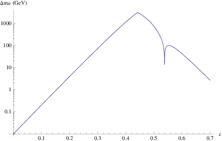
Let us now redetermine the correction to the Higgs mass due to hypermultiplets using propagators. This takes the contributions from all KK modes (and the zero-modes) into account. As before, we will assume that both hypermultiplets in the Yukawa coupling to the Higgs have the same -value and we will only take the SUSY-breaking mass on the UV brane into account.1919 19 In absence of SUSY breaking in the bulk, the KK modes effectively lower the cutoff from the new-physics scale to the IR scale [17]. This follows simply from the fact that, with SUSY being only broken on the UV brane, loop corrections on the IR brane are UV-finite by locality and therefore cannot depend on the cutoff . It is an interesting question whether the cutoff is still lowered if SUSY is broken in the bulk by the spurion . In mixed position-momentum representation and evaluated on the IR brane, the propagators of the fermion and the scalar are given by [17]
| (78) |
where is the momentum and we restrict ourselves to . Here and are the modified Bessel functions and for is defined as
| (79) |
and similarly for . For the scalar, and whereas for the fermion . The one-loop correction to the Higgs mass is then given by [17]
| (80) |
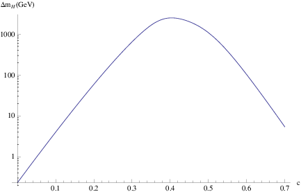
where is the Yukawa coupling and we have assumed that the fermionic zero-mode is a quark. In Fig. 3, we have plotted the correction for the case , and . Note in particular that our estimate in Fig. 2 reproduces the result in Fig. 3 reasonably well. We see that the correction becomes relatively large for -values close to . More precisely, if we want at most tuning for a Higgs mass of , we must exclude -values between and . We do not expect that this is a problem for successful phenomenology: The statistical analysis performed in [33] to determine the -values that ‘most naturally’ reproduce the quark masses and the CKM matrix finds two -values which are marginally in that range, for the top-bottom doublet and for the right-handed charm. But we have already discussed in Sect. 3.1 that there is some freedom in choosing these -values. Note furthermore that in our calculation we have assumed that the left- and right-handed hypermultiplet have the same . We expect that, if only one of both hypermultiplets lies in the region , the correction will be smaller.
Next, we will discuss loop corrections to the Higgs mass from the gauge sector. Since the SUSY-breaking gaugino masses in the bulk and on the branes are at most of order , we can restrict our discussion to the zero-modes from the vector multiplets. Light gauginos, however, are not enough to guarantee that these corrections are sufficiently small: The superpartners of the first two generations obtain high masses and can be integrated out below that scale. Without their superpartners, the first-two-generation fermions only renormalize the gauge couplings and not the couplings involving gauginos or -terms (at one-loop). This induces a (hard SUSY-breaking) mismatch between these couplings and thereby gives a contribution to scalar masses in the IR [18],
| (81) |
where respectively for and . The parameter is the anomalous dimension of the -term-squared in the dual picture (see [18] for more details). As in [18], we will take and as well as and . Choosing and , we find the following contributions to stop and Higgs masses:2020 20 In contrast to the findings of [13, 14], these contributions are relatively small even when the first-two-generation superpartners have masses around . The reason is that our cutoff is low and that the CFT (in the dual picture) provides a focussing effect for the vector multiplet couplings [18].
| (82) |
A stop mass (as motivated in Sect. 4) thus requires a tuning in the -range of this contribution against the gravity-mediated soft mass. The contribution to the Higgs mass in Eq. (82) in turn is negligible compared to that from stop loops (which again introduce a tuning of order for , see Sect. 4). Both contributions in Eq. (82) can be reduced with a lower cutoff or with smaller .
There is a potentially large correction to the Higgs mass from a -term which forces us to extend the gauge group of the standard model as we will now discuss [39, 18]: Recall first that a bulk vector multiplet consists of a vector multiplet and a chiral multiplet of SUSY. The -term in is related to the scalar in according to [29]
| (83) |
where the ellipsis denote contributions from bulk hypermultiplets and brane-localized chiral multiplets. A term linear in on the UV brane, if induced by broken SUSY, causes the profile of the scalar in to grow rapidly towards the IR. This leads to excessive SUSY breaking in the IR. To ensure the absence of terms linear in , the -terms have to carry a charge. In the standard model, however, the hypercharge -term is not charged under any symmetry. We therefore have to extend the standard model group [12, 18]. One possibility is a semi-simple GUT since -terms for nonabelian gauge groups are in the adjoint representation. Another possibility is the left-right model of [40]2121 21 This model has the gauge group and a discrete parity symmetry. In the simplest realization, one would assign right-handed standard model fields to doublets of . Since bulk fields in the same doublet have the same mass parameter , it may however be difficult to obtain the right Yukawa couplings without some hierarchy in the Yukawa couplings. Alternatively, one may introduce additional particles to fill up the doublets. in which the abelian -term obtains a discrete charge.2222 22 Similarly, we have to ensure that the -term of the (see Sect. 3.1) has a discrete charge. Alternatively, we can replace the by a nonabelian gauge symmetry. This extended symmetry moreover ensures that
| (84) |
where denotes the hypercharge of the -th scalar and the mass matrices of scalar superpartners on the right-hand side are -matrices in family space, and thereby that -term interactions give sufficiently small contributions to the Higgs mass (see e.g. [41]). In the following, we will assume such an extension of the standard model. We will furthermore assume that the extended group is broken down to the standard model at the IR scale, leading to additional gauge bosons with masses around that scale.
Let us now see how the little hierarchy between TeV and the electroweak scale,
| (85) |
can be generated in our model. Recall from Eq. (46) that the hierarchy between the IR scale and the soft scale is determined by the quantity . The soft scale in turn sets the scale of dimensionful parameters in the Higgs potential and thereby controls the scale of electroweak symmetry breaking. For definiteness, we will set . The little hierarchy in Eq. (85) then follows from a very modest hierarchy between and :
| (86) |
To summarize, stops, gauginos and Higgsinos protect the Higgs from the cutoff down to the electroweak scale. We estimate that the residual tuning required to obtain the correct -mass for is in the -range. The little hierarchy between the cutoff and the electroweak scale is controlled by the quantity which can be large already for very modest hierarchies between and due to the appearance of the third power.
6 Electroweak and Flavour Constraints
Let us briefly discuss various constraints on our model, beginning with electroweak precision tests. Important constraints arise from the Peskin-Takeuchi parameters and and the -coupling. In warped models with low KK mass scale, a custodial symmetry is required to satisfy these constraints. But for our TeV (see Sect. 5), the KK modes have masses of at least . This high scale ensures that corrections to and the -coupling from KK modes are sufficiently small even without a custodial symmetry [42]. But we similarly have to check whether no excessive corrections arise from the light modes. In particular, we want a heavy Higgs to minimize fine-tuning. For large Higgs-singlet coupling , the Higgs mass can be as large as 300 GeV (cf. Sect. 4). By itself, such a heavy Higgs would be incompatible with electroweak precision tests. The contributions to and from the scalars and fermions in the Higgs sector, stops and sbottoms were determined in [23], assuming that the gauginos are sufficiently heavy to be neglected (cf. Sect. 4). It turns out that the contribution from a heavy Higgs is cancelled by the other Higgs sector particles (whose contributions are enhanced for large ) for and that most of the parameter space is brought into the region of the ellipse preferred by experiment. This is another reason why we focus on small in this work.
In addition, important constraints arise from flavour- and -violating processes. Extensive studies of such processes in warped models with bulk fermions were undertaken in [5, 6] (see [7] for a review and additional references). It was found that the strongest constraints arise from the electric dipole moment of the neutron and violation in Kaons. In particular, these constraints require respectively that [5] and [7], where sets the overall scale of Yukawa couplings in units of . The fact that these constraints cannot be fulfilled for low KK mass scales is known as the RS problem [5]. But assuming that (which still allows for one or two KK levels before the Yukawa couplings become strongly coupled, see e.g. [7]), our KK mass scale of is sufficiently high.
This ensures that KK modes of standard model fermions and gauge bosons do not lead to excessive flavour and violation. But in our supersymmetric model, we also have to consider contributions from their superpartners. As we have discussed in the introduction, we avoid the flavour problem of the MSSM by raising the masses of the first-two-generation sparticles above 1000 TeV. Compared with fermionic and gauge KK modes, higher KK modes of scalar superpartners have two additional sources of flavour and violation: 1) Gravity mediation in the bulk leads to flavour-violating masses of order . 2) Assuming that the messenger sector on the UV brane is not flavour-blind, there are large flavour-violating masses on the UV brane.2323 23 An alternative possibility is a flavour-blind mechanism such as gauge mediation. An -sym-metric version (so that gauginos remain light even when the SUSY-breaking scale is high) of gauge mediation has been presented in [43]. As we have seen in Eq. (74), the wavefunction overlap of scalar KK modes with the UV brane can be large, meaning that they may obtain large flavour-violating masses from the UV brane.
Let us assume that flavour is maximally violated by the masses of scalar KK modes. This is a very conservative assumption as the wavefunction overlap with the UV brane is large only for close to . We will now show that even then flavour- and -violating processes mediated by scalar KK modes are sufficiently small. We first consider processes which contribute to - and - mixing. The leading RS diagram is tree-level KK gluon exchange[5], whereas the SUSY diagrams are at loop level. The SUSY diagrams have the same flavour structure as the tree-level diagrams and are therefore loop-suppressed compared to the KK gluon exchange; the tree-level process itself is sufficiently small for . Next are the processes, such as , , and . For the RS diagrams are again tree-level while the SUSY diagrams are loop-suppressed. The process is suppressed relative to the SM diagrams by a factor (where is the effective -term, see Sect. 4). The process , finally, occurs at one-loop in both RS models and SUSY models; however, the dimension- operators require a chirality flip which for SUSY scalars can only originate from -terms or the SUSY Higgs mass times a Yukawa coupling. The -terms can never be large in our model as the Higgs is confined to the IR brane and they are protected by an approximate -symmetry. Consequently, the remaining SUSY scalar diagrams are identical to those of KK gluon exchange [5] except that the scalar diagrams come with a suppression factor of . The dimension- operators for do not require a chirality flip, but they are also sufficiently small for . An additional concern is from new violation—particularly from contributions to and the neutron’s electric dipole moment [5, 7]. For , the RS processes are sufficiently suppressed [5, 7]; meanwhile, as these -violating effects require a chirality flip, the SUSY diagrams are again suppressed relative to the RS graphs by at least .
7 Conclusions
A warped extra dimension and supersymmetry are popular solutions to the hierarchy problem. In addition, a warped extra dimension allows the fermion mass hierarchy to be naturally generated. Both however are not without issues: In Randall-Sundrum models, the IR scale has to be chosen much larger than the electroweak scale to satisfy phenomenological constraints, leading to a little hierarchy problem. In the MSSM, on the other hand, the tree-level Higgs mass is below the LEP bound. To raise this mass radiatively, heavy stops are required, again causing a little hierarchy problem. Additional issues in the MSSM are the flavour problem of supersymmetry breaking and the -problem.2424 24 Of course, various solutions to all these problems exist. But often these solutions are plagued by other problems (the tachyonic-slepton problem in anomaly mediation or the -problem in gauge mediation) or require complicated additional structure (such as flavour symmetries or custodial symmetries in Randall-Sundrum models). We have shown that the combination of a warped extra dimension and supersymmetry can lead to a model where these problems are naturally avoided. Such a combination seems natural in light of string realizations of the Randall-Sundrum model [44].
More precisely, we have shown how to generate and stabilize a little hierarchy between the IR scale and the electroweak scale in a supersymmetric Randall-Sundrum model. This allows for an IR scale around 10 TeV without causing excessive fine-tuning. The resulting Kaluza-Klein scale is sufficiently heavy to comply with all phenomenological constraints (in particular from violation) on Randall-Sundrum models without the need to introduce custodial or flavour symmetries.
To this end, the warped extra dimension is stabilized by a bulk hypermultiplet and a constant superpotential on the IR brane. Supersymmetry is broken on the UV brane [17], leading to a superparticle spectrum where the first-two generation squarks and sleptons are above 1000 TeV. This avoids the supersymmetric flavour and problems. The gaugino is protected by an accidental -symmetry [18] but eventually obtains a mass close to the electroweak scale from either radion mediation or a suppressed operator on the UV brane. The bulk hypermultiplet moreover obtains an -term from the UV brane and induces soft masses near the IR brane for stops, sbottoms and the Higgs sector. The resulting soft scale can naturally be a factor below the IR scale, thereby generating a little hierarchy between both scales. This little hierarchy is stabilized against radiative corrections by stops, gauginos and Higgsinos, which are the only superpartners in the low-energy spectrum apart from sbottoms and possibly the gravitino. This is reminiscent of the particle content in the more minimal supersymmetric standard model and related scenarios [11, 12].
To alleviate the supersymmetric little hierarchy problem, the Higgs sector on the IR brane is extended with the inclusion of a singlet, as in the NMSSM. This yields an additional contribution to the Higgs quartic coupling and can therefore raise the Higgs mass already at tree-level. Since we have to require perturbativity of the Higgs-singlet coupling only up to the IR scale, this effect can be much larger than in the NMSSM. Tuning is further reduced because the Higgs can be relatively heavy. In addition, log-factors from loop integrals are relatively small due to the low cutoff. We have given an example where the residual tuning to obtain the correct -mass is in the -range. Examples with even less tuning may also be possible. Similar to the NMSSM, the singlet moreover provides a solution to the -problem. To avoid a large -term contribution to soft masses the model must be embedded into a GUT group. This allows for the possibility of gauge coupling unification as considered in Ref. [45]. Finally, the LSP is dominantly Higgsino in a well-motivated region of parameter space. This Higgsino LSP is a viable dark matter candidate.
In the dual interpretation the Higgs sector is composite. This protects the Higgs mass from the Planck scale to the IR scale of order 10 TeV. The remaining little hierarchy between the IR scale and the electroweak scale is explained by accidental supersymmetry at low energies. Supersymmetry breaking occurs in the elementary sector and is transmitted to the composite sector by marginal or marginally irrelevant operators. The stabilization of the warped extra dimension requires a constant IR superpotential which can be thought of as a gaugino condensate in a Seiberg dual theory. It is beyond the scope of this work, but it would be worth exploring the dual interpretation further.
Let us finally comment on the relevance of our model for the LHC. The low-energy spectrum accessible to the LHC has similarities with other realizations of SUSY [23, 24, 25, 26]: We expect a relatively heavy Higgs and likely have a Higgsino LSP. The only other light standard model superpartners (apart from the Higgsinos) are stops, sbottoms and gauginos. But we also have specific predictions: Soft masses for the Higgs sector, stops and sbottoms result from gravity mediation at the IR scale of order . The dominant source of -breaking soft terms, on the other hand, are the gaugino masses. In particular, -terms are generated mainly radiatively. It would be interesting to study electroweak symmetry breaking under these conditions and to see whether further predictions on the spectrum can be obtained. In addition, a radion (and possibly its fermionic superpartner) around the soft scale is a unique prediction of our model compared to general SUSY scenarios and could be discovered at the LHC. Higher KK modes and the remaining superpartners, on the other hand, may only be accessible to next-generation colliders.
Acknowledgments
We thank Arthur Hebecker, Shrihari Gopalakrishna and Michael G. Schmidt for helpful discussions. This work is supported by the Australian Research Council. TG thanks the SITP at Stanford for support and hospitality during the completion of this work. BvH and NS thank SLAC for hospitality during the final stages of this project.
Appendix A Radion stabilization for generic SUSY-breaking potentials
Here we shall discuss the minimization of the radion potential for general SUSY-breaking potentials . We will see that we obtain essentially the same minimum as given in Sect. 2.
Using the general wavefunctions Eqs. (8)–(10) and the boundary conditions Eq. (12), we first find that the wavefunctions take the simpler form
| (87) |
The remaining integration constants and are determined by the boundary conditions
| (88) |
According to the assumption discussed in Sect. 2, each and comes with a factor in the SUSY-breaking potential and the only other scale involved is the SUSY-breaking scale . It is convenient to write the SUSY-breaking potential as a dimensionless function of the rescaled fields and . The boundary conditions then take the form
| (89) |
We are interested in the potential for . It is therefore sufficient to solve for and as power series in . From Eq. (89), we conclude that these power series take the form (assuming ):
| (90) |
For a generic function , the dimensionless coefficients etc. will generically be of order one. Returning to the unrescaled variables, we see that then the coefficients in the expansion of are of order and those for are of order .
To determine the radion potential, we also need to know . Using Eq. (87) and the power series, we find
| (91) |
Expanding the SUSY-breaking potential in and using Eqs. (88) and (90), we similarly find
| (92) |
We now have all the necessary results to evaluate the effective potential given in Eq. (13). To determine the dependence on the scalar superpartner of the radion, we promote the radion to a chiral superfield via analytic continuation into superspace [30, 28]. Performing the -integral, the potential in Eq. (13) depends on the lowest component of this chiral superfield which we again denote by . Including the contribution from the constant superpotential on the IR brane in Eq. (20), we find for the -dependent part of the potential
| (93) |
where
| (94) |
We see that, with the replacements and , this potential is identical to the potential Eq. (21). Its minimum is accordingly given by Eq. (22) with the replacement . Since the coefficients in the expansion of are generically of order as argued before, we find that . The minimum thus has the same dependence on the SUSY-breaking scale as before.
Let us now consider the constant part of the effective potential. Including the contribution from the constant superpotential on the UV brane in Eq. (20), it reads
| (95) |
From Eq. (89), we expect that in the minimum for a generic function . The first two terms in Eq. (95) are then of order . Assuming that their contribution to the effective potential is positive, to tune the cosmological constant to zero we have to choose
| (96) |
The expansion leading to Eq. (93) breaks down in the region . We have to check whether the energy density in this region is not smaller than in the minimum Eq. (22). When , however, the energy density from the constant superpotential on the IR brane is of order . Since we assume that , this is much larger than the energy density in the minimum Eq. (22). We thus find that this minimum is again the global minimum.
Appendix B A simple messenger sector on the UV brane
Here we will present a simple messenger sector on the UV brane. For simplicity, we will only discuss messengers which couple to left-handed squarks (or the corresponding chiral multiplets). There will be corresponding messengers with the right quantum numbers to couple to the remaining squarks and sleptons. More precisely, we consider messengers , , and whose charge assignments under the standard model gauge group and the are given in Table 1.
Furthermore, is the spurion and we have suppressed the family index for the left-handed quark superfields . The charge assignments allow for the superpotential
| (97) |
where is a mass scale. Integrating out the messengers generates the coupling in Eq. (34) (up to a loop factor). The -violating coupling in Eq. (36), on the other hand, is not generated as the messenger sector preserves the accidental -symmetry. This follows from the following -charge assignments:
| (98) |
It is straightforward to include messengers for the other squarks and sleptons in a way that either preserves or breaks the accidental -symmetry.
References
- [1] L. Randall and R. Sundrum, Phys. Rev. Lett. 83 (1999) 3370 [arXiv:hep-ph/9905221].
- [2] Y. Grossman and M. Neubert, Phys. Lett. B 474 (2000) 361 [arXiv:hep-ph/ 9912408].
- [3] T. Gherghetta and A. Pomarol, Nucl. Phys. B 586 (2000) 141 [arXiv:hep-ph/0003129].
- [4] S. J. Huber, Q. Shafi, Phys. Lett. B498, 256-262 (2001). [hep-ph/0010195].
- [5] K. Agashe, G. Perez and A. Soni, Phys. Rev. Lett. 93 (2004) 201804 [arXiv:hep-ph/0406101]; K. Agashe, G. Perez and A. Soni, Phys. Rev. D 71 (2005) 016002 [arXiv:hep-ph/0408134].
- [6] M. Bona et al. [UTfit Collaboration], JHEP 0803 (2008) 049 [arXiv:0707.0636 [hep-ph]]; K. Agashe et al., Phys. Rev. D 76 (2007) 115015 [arXiv:0709.0007 [hep-ph]]; C. Csaki, A. Falkowski and A. Weiler, JHEP 0809 (2008) 008 [arXiv:0804.1954 [hep-ph]].
- [7] G. Isidori, Y. Nir and G. Perez, arXiv:1002.0900 [hep-ph] and references therein.
- [8] A. L. Fitzpatrick, G. Perez and L. Randall, arXiv:0710.1869 [hep-ph]; A. L. Fitzpatrick, L. Randall and G. Perez, Phys. Rev. Lett. 100 (2008) 171604; C. Csaki, A. Falkowski and A. Weiler, Phys. Rev. D 80 (2009) 016001 [arXiv:0806.3757 [hep-ph]]; J. Santiago, JHEP 0812 (2008) 046 [arXiv:0806.1230 [hep-ph]]; C. Csaki, G. Perez, Z. Surujon and A. Weiler, Phys. Rev. D 81 (2010) 075025 [arXiv:0907.0474 [hep-ph]]; M. C. Chen, K. T. Mahanthappa and F. Yu, Phys. Rev. D 81 (2010) 036004 [arXiv:0907.3963 [hep-ph]].
- [9] R. Barbieri and A. Strumia, arXiv:hep-ph/0007265.
- [10] N. Arkani-Hamed, A. G. Cohen and H. Georgi, Phys. Lett. B 513 (2001) 232 [arXiv:hep-ph/0105239].
- [11] M. Dine, A. Kagan and S. Samuel, Phys. Lett. B 243 (1990) 250; M. Dine, R. G. Leigh and A. Kagan, Phys. Rev. D 48 (1993) 4269 [arXiv:hep-ph/9304299]; P. Pouliot and N. Seiberg, Phys. Lett. B 318 (1993) 169 [arXiv:hep-ph/9308363]; A. Pomarol and D. Tommasini, Nucl. Phys. B 466 (1996) 3 [arXiv:hep-ph/9507462]; R. Barbieri, G. R. Dvali and L. J. Hall, Phys. Lett. B 377 (1996) 76 [arXiv:hep-ph/9512388]; R. Barbieri, L. J. Hall and A. Romanino, Phys. Lett. B 401 (1997) 47 [arXiv:hep-ph/9702315].
- [12] A. G. Cohen, D. B. Kaplan and A. E. Nelson, Phys. Lett. B 388 (1996) 588 [arXiv:hep-ph/9607394];
- [13] R. Barbieri and G. F. Giudice, Nucl. Phys. B 306 (1988) 63; S. Dimopoulos and G. F. Giudice, Phys. Lett. B 357 (1995) 573 [arXiv:hep-ph/9507282].
- [14] N. Arkani-Hamed, H. Murayama, Phys. Rev. D56 (1997) 6733-6737. [hep-ph/9703259].
- [15] G. F. Giudice, M. Nardecchia and A. Romanino, Nucl. Phys. B 813 (2009) 156 [arXiv:0812.3610 [hep-ph]];
- [16] R. Barbieri, E. Bertuzzo, M. Farina, P. Lodone and D. Pappadopulo, JHEP 1008 (2010) 024 [arXiv:1004.2256 [hep-ph]].
- [17] T. Gherghetta and A. Pomarol, Phys. Rev. D 67 (2003) 085018 [arXiv:hep-ph/0302001].
- [18] R. Sundrum, JHEP 1101 (2011) 062. [arXiv:0909.5430 [hep-th]].
- [19] A. Kehagias and K. Tamvakis, Phys. Lett. B 504 (2001) 38 [arXiv:hep-th/0010112]; B. Batell and T. Gherghetta, Phys. Rev. D 73 (2006) 045016 [arXiv:hep-ph/0512356]; T. Gherghetta and B. von Harling, JHEP 1004 (2010) 039 [arXiv:1002.2967 [hep-ph]].
- [20] N. Arkani-Hamed and S. Dimopoulos, JHEP 0506 (2005) 073 [arXiv:hep-th/0405159].
- [21] N. Arkani-Hamed, S. Dimopoulos, G. F. Giudice and A. Romanino, Nucl. Phys. B 709 (2005) 3 [arXiv:hep-ph/0409232].
- [22] M. Redi and B. Gripaios, JHEP 1008 (2010) 116 [arXiv:1004.5114 [hep-ph]].
- [23] R. Barbieri, L. J. Hall, Y. Nomura and V. S. Rychkov, Phys. Rev. D 75 (2007) 035007 [arXiv:hep-ph/0607332].
- [24] R. Franceschini and S. Gori, arXiv:1005.1070 [hep-ph].
- [25] R. Kitano, G. D. Kribs and H. Murayama, Phys. Rev. D 70 (2004) 035001 [arXiv:hep-ph/0402215]; L. Cavicchia, R. Franceschini and V. S. Rychkov, Phys. Rev. D 77 (2008) 055006 [arXiv:0710.5750 [hep-ph]]; J. Cao and J. M. Yang, Phys. Rev. D 78 (2008) 115001 [arXiv:0810.0989 [hep-ph]]; P. Lodone, JHEP 1005 (2010) 068 [arXiv:1004.1271 [hep-ph]].
- [26] R. Harnik, G. D. Kribs, D. T. Larson and H. Murayama, Phys. Rev. D 70 (2004) 015002 [arXiv:hep-ph/0311349]; A. Birkedal, Z. Chacko and Y. Nomura, Phys. Rev. D 71 (2005) 015006 [arXiv:hep-ph/0408329].
- [27] R. Altendorfer, J. Bagger and D. Nemeschansky, Phys. Rev. D 63 (2001) 125025 [arXiv:hep-th/0003117].
- [28] H. S. Goh, M. A. Luty and S. P. Ng, JHEP 0501 (2005) 040 [arXiv:hep-th/ 0309103].
- [29] D. Marti and A. Pomarol, Phys. Rev. D 64 (2001) 105025 [arXiv:hep-th/ 0106256].
- [30] M. A. Luty and R. Sundrum, Phys. Rev. D 64 (2001) 065012 [arXiv:hep-th/ 0012158].
- [31] S. A. Abel, S. Sarkar and P. L. White, Nucl. Phys. B 454 (1995) 663 [arXiv:hep-ph/9506359].
- [32] S. A. Abel, Nucl. Phys. B480 (1996) 55-72. [hep-ph/9609323]; C. Panagio-takopoulos and K. Tamvakis, Phys. Lett. B 446 (1999) 224 [arXiv:hep-ph/9809475];
- [33] S. J. Huber, Nucl. Phys. B 666 (2003) 269 [arXiv:hep-ph/0303183].
- [34] Z. Chacko and M. A. Luty, JHEP 0105 (2001) 067 [arXiv:hep-ph/0008103].
- [35] M. A. Luty, Phys. Rev. Lett. 89 (2002) 141801 [arXiv:hep-th/0205077].
- [36] U. Ellwanger, C. Hugonie and A. M. Teixeira, Phys. Rept. 496 (2010) 1 [arXiv:0910.1785 [hep-ph]].
- [37] S. Mizuta, M. Yamaguchi, Phys. Lett. B298 (1993) 120-126. [hep-ph/9208251].
- [38] R. Dermisek, J. F. Gunion, Phys. Rev. Lett. 95 (2005) 041801. [hep-ph/0502105]; R. Dermisek, J. F. Gunion, Phys. Rev. D75 (2007) 075019. [hep-ph/0611142].
- [39] M. J. Strassler, arXiv:hep-th/0309122.
- [40] R. N. Mohapatra and J. C. Pati, Phys. Rev. D 11 (1975) 2558; G. Senjanovic and R. N. Mohapatra, Phys. Rev. D 12 (1975) 1502.
- [41] S. P. Martin, In *Kane, G.L. (ed.): Perspectives on supersymmetry* 1-98. [hep-ph/9709356].
- [42] H. Davoudiasl, S. Gopalakrishna, E. Ponton and J. Santiago, New J. Phys. 12 (2010) 075011 [arXiv:0908.1968 [hep-ph]] and references therein.
- [43] S. D. L. Amigo, A. E. Blechman, P. J. Fox and E. Poppitz, JHEP 0901 (2009) 018 [arXiv:0809.1112 [hep-ph]].
- [44] I. R. Klebanov, M. J. Strassler, JHEP 0008, 052 (2000). [hep-th/0007191]; S. B. Giddings, S. Kachru, J. Polchinski, Phys. Rev. D66, 106006 (2002). [hep-th/0105097].
- [45] T. Gherghetta, Phys. Rev. D71, 065001 (2005). [hep-ph/0411090]; K. Agashe, R. Contino, R. Sundrum, Phys. Rev. Lett. 95, 171804 (2005). [hep-ph/0502222].