跳到论文正文
W Papers独立论文阅读器 arXiv:1104.3138 论文正文 计算阅读时间 · 0%
引用这篇论文根据当前论文元数据生成,正式投稿前建议核对。


License: arXiv.org perpetual non-exclusive license
arXiv:1104.3138v2 [hep-ph] 21 Jun 2011

O⁡(αs​v2)O(\alpha_{s}v^{2}) Corrections to Hadronic and Electromagnetic Decays of S01{}^{1}{S}_{0} Heavy Quarkonium

Huai-Ke Guo Email: huaike.guo@gmail.com Affiliation: Department of Physics and State Key Laboratory of Nuclear Physics and Technology, Peking University, Beijing 100871, China    Yan-Qing Ma Email: yqma.cn@gmail.com Affiliation: Department of Physics and State Key Laboratory of Nuclear Physics and Technology, Peking University, Beijing 100871, China    Kuang-Ta Chao Email: ktchao@th.phy.pku.edu.cn Affiliation: Department of Physics and State Key Laboratory of Nuclear Physics and Technology, and Center for High Energy Physics,
Peking University, Beijing 100871, China
Abstract

We study O⁡(αs​v2)O(\alpha_{s}v^{2}) corrections to decays of S01{}^{1}S_{0} heavy quarkonium into light hadrons and two photons within the framework of nonrelativistic QCD (NRQCD), and find these O⁡(αs​v2)O(\alpha_{s}v^{2}) corrections to have significant contributions especially for the decay into light hadrons. With these new results, experimental measurements of the hadronic width and the γ​γ\gamma\gamma width of ηc\eta_{c} can be described more consistently. By fitting experimental data, we find the long-distance matrix elements of ηc\eta_{c} to be |ℛηc​(0)|2=0.834−0.197+0.281​GeV3|\mathcal{R}_{\eta_{c}}(0)|^{2}=0.834^{+0.281}_{-0.197}\ \textrm{GeV}^{3} and ⟨𝒗2⟩ηc=0.232−0.098+0.121\langle\bm{v}^{2}\rangle_{\eta_{c}}=0.232^{+0.121}_{-0.098}. Moreover, ηc​(2​S)\eta_{c}(2S) is also discussed and the γ​γ\gamma\gamma decay width is predicted to be 3.34−2.10+2.06​KeV3.34^{+2.06}_{-2.10}\ \textrm{KeV}.

pacs
12.38.Bx, 13.20.Gd, 14.40.Pq

I Introduction

Heavy quarkonium plays an important role in establishing and understanding quantum chromodynamics (QCD), the fundamental theory of strong interactions. Due to the existence of several energy scales involved with these systems, heavy quarkonium provides an ideal laboratory for testing the perturbative and nonperturbative effects of QCD. An effective theory suitable for describing these systems is nonrelativistic QCD (NRQCD)[1], which is derived from QCD by considering the underlying nonrelativistic properties. According to NRQCD factorization[2], decays of heavy quarkonium into light hadrons or photons can be organized in a hierarchy of long-distance matrix elements (LDMEs), which are classified in terms of vv, the relative velocity of the heavy quarks in heavy quarkonium.

Decays of S01{}^{1}{S}_{0} heavy quarkonium into light hadrons (LH) and two photons are among the simplest processes. The short-distance coefficients for corresponding LDMEs at leading order in vv have been computed previously to next-to-leading order (NLO) in αs\alpha_{s} [3, 4, 5, 2, 6, 7, 8, 9, 10, 11, 12]. Moreover, that coefficient for γ​γ\gamma\gamma decay has been calculated to next-to-next-to-leading order (NNLO) in αs\alpha_{s} [13]. However, all coefficients of LDMEs beyond leading order in vv are known at best to leading order in αs\alpha_{s} [14, 6, 15, 16]. It is well known that the calculation at leading order in αs\alpha_{s} suffers from large uncertainties due to strong renormalization scale dependence. Therefore, to give a more precise description for S01{}^{1}{S}_{0} heavy quarkonium decays beyond leading order in vv, QCD corrections to these coefficients are apparently needed.

In this paper, we will study QCD corrections to the coefficients of order v2v^{2} LDME, namely, corrections at order αs​v2\alpha_{s}v^{2} for S01{}^{1}{S}_{0} quarkonium decays. Up to this order of corrections, there are two unknown LDMEs which should be fixed. Unfortunately, lattice calculation of these LDMEs [17, 18], though based on first principles, suffers from large uncertainties. In Refs.[19, 20, 21], a new method was introduced to estimate LDMEs by combining potential models, lattice calculation, and experimental data. This method will also be used in this paper to determine the two unknown LDMEs. Then with our calculated αs​v2\alpha_{s}v^{2} corrections we will be able to get updated estimates for the decay widths of S01{}^{1}{S}_{0} heavy quarkonium into light hadrons and two photons.

The rest of this paper is organized as follows. We briefly introduce the theoretical procedures for calculations of heavy quarkonium decays in Sec. II. In Sec. III, we describe kinematics and method of calculation for these processes. Results in perturbative QCD are summarized in Sec. IV, while corresponding results in perturbative NRQCD are summarized in Sec. V. By using the matching condition, we give the updated short distance coefficients in Sec.VI to include our new αs​v2\alpha_{s}v^{2} corrections. With these newly obtained results, we determine the two unknown LDMEs using potential models and make predictions for relevant decay widths in Sec. VII. Finally, in Sec. VIII, we present a brief summary.

II Decay of Heavy Quarkonium in NRQCD

The Lagrangian of NRQCD is derived from the QCD Lagrangian by integrating out the degrees of freedom of order mQm_{Q}, the mass of the heavy quark. Local 4-fermion operators are added to accommodate the inclusive annihilation decay of heavy quarkonium which happens at scale of order mQm_{Q}. The Lagrangian of NRQCD is

ℒNRQCD=ℒlight+ℒheavy+δ​ℒ.\mathcal{L}_{\textrm{NRQCD}}=\mathcal{L}_{\textrm{light}}+\mathcal{L}_{\textrm{heavy}}+\delta\mathcal{L}. (1)

Here ℒheavy\mathcal{L}_{\textrm{heavy}} describes nonrelativistic heavy quarks and antiquarks and is given by

ℒheavy=ψ†​(i​Dt+𝐃22​mQ)​ψ+χ†​(i​Dt−𝐃22​mQ)​χ,{\mathcal{L}}_{\textrm{heavy}}\;=\;\psi^{\dagger}\,\left(iD_{t}+\frac{{\bf D}^{2}}{2m_{Q}}\right)\,\psi\;+\;\chi^{\dagger}\,\left(iD_{t}-\frac{{\bf D}^{2}}{2m_{Q}}\right)\,\chi, (2)

where ψ\psi is the Pauli spinor field that annihilates a heavy quark, χ\chi is the Pauli spinor field that creates a heavy antiquark and DtD_{t} and 𝐃{\bf D} are the time and space components of the gauge-covariant derivative DμD^{\mu}. Terms corresponding to light quarks and gluons are given by ℒlight{\mathcal{L}}_{\textrm{light}} and

ℒlight=−12​tr​Gμ​ν​Gμ​ν+∑q¯​i​​D​q,{\mathcal{L}}_{\textrm{light}}\;=\;-{1\over 2}{\textrm{tr}}\,G_{\mu\nu}G^{\mu\nu}\;+\;\sum\bar{q}\;i{\not\!\!D}q, (3)

where Gμ​νG_{\mu\nu} is the gluon field strength tensor, qq is the Dirac spinor field for light quarks and the sum is over nfn_{f} flavors of light quarks. Relativistic corrections to the basic effective lagrangian ℒheavy+ℒlight\mathcal{L}_{\textrm{heavy}}+\mathcal{L}_{\textrm{light}} are included in δ​ℒ\delta\mathcal{L} and its leading terms are those bilinear in the heavy quark or antiquark field,

δ​ℒbilinear\displaystyle\delta{\mathcal{L}}_{\textrm{bilinear}} =\displaystyle= c18​mQ3​(ψ†​(𝐃2)2​ψ−χ†​(𝐃2)2​χ)\displaystyle\frac{c_{1}}{8m_{Q}^{3}}\left(\psi^{\dagger}({\bf D}^{2})^{2}\psi\;-\;\chi^{\dagger}({\bf D}^{2})^{2}\chi\right) (4)
+\displaystyle+ c28​mQ2​(ψ†​(𝐃⋅g​𝐄−g​𝐄⋅𝐃)​ψ+χ†​(𝐃⋅g​𝐄−g​𝐄⋅𝐃)​χ)\displaystyle\frac{c_{2}}{8m_{Q}^{2}}\left(\psi^{\dagger}({\bf D}\cdot g{\bf E}-g{\bf E}\cdot{\bf D})\psi\;+\;\chi^{\dagger}({\bf D}\cdot g{\bf E}-g{\bf E}\cdot{\bf D})\chi\right)
+\displaystyle+ c38​mQ2​(ψ†​(i​𝐃×g​𝐄−g​𝐄×i​𝐃)⋅𝝈​ψ+χ†​(i​𝐃×g​𝐄−g​𝐄×i​𝐃)⋅𝝈​χ)\displaystyle\frac{c_{3}}{8m_{Q}^{2}}\left(\psi^{\dagger}(i{\bf D}\times g{\bf E}-g{\bf E}\times i{\bf D})\cdot\mbox{\boldmath$\sigma$}\psi\;+\;\chi^{\dagger}(i{\bf D}\times g{\bf E}-g{\bf E}\times i{\bf D})\cdot\mbox{\boldmath$\sigma$}\chi\right)
+\displaystyle+ c42​mQ​(ψ†​(g​𝐁⋅𝝈)​ψ−χ†​(g​𝐁⋅𝝈)​χ),\displaystyle\frac{c_{4}}{2m_{Q}}\left(\psi^{\dagger}(g{\bf B}\cdot\mbox{\boldmath$\sigma$})\psi\;-\;\chi^{\dagger}(g{\bf B}\cdot\mbox{\boldmath$\sigma$})\chi\right),

where Ei=G0​iE^{i}=G^{0i} and Bi=12​ϵi​j​k​Gj​kB^{i}=\mbox{$\frac{1}{2}$}\epsilon^{ijk}G^{jk} are the electric and magnetic components of the gluon field strength tensor Gμ​νG^{\mu\nu}.

Further corrections include the description of inclusive annihilation decay of heavy quarkonium and can be achieved by adding local 4-fermion interactions as

δ​ℒ4-fermion=∑nfn​(μΛ)mQdn−4​𝒪n​(μΛ),\delta{\mathcal{L}}_{\textrm{4-fermion}}\;=\;\sum_{n}{\frac{f_{n}(\mu_{\Lambda})}{m_{Q}^{d_{n}-4}}}{\mathcal{O}}_{n}(\mu_{\Lambda}), (5)

where μΛ\mu_{\Lambda} is the NRQCD factorization scale, 𝒪n​(μΛ)\mathcal{O}_{n}(\mu_{\Lambda}) is the local 4-fermion operator, dnd_{n} is the naive scaling dimension of the operator and fn​(μΛ)f_{n}(\mu_{\Lambda}) is the short-distance coefficient which can be calculated perturbatively.

Thus the decay width of heavy quarkonium can be given by the following factorization formula

Γ⁡(H)=∑n2​Im​fn​(μΛ)mQdn−4​⟨H|​𝒪n​(μΛ)​|H⟩,\Gamma(H)=\sum_{n}\frac{2\textrm{Im}f_{n}(\mu_{\Lambda})}{m_{Q}^{d_{n}-4}}\langle H|\mathcal{O}_{n}(\mu_{\Lambda})|H\rangle, (6)

where heavy quarkonium state in the Fock space can be written as [2]

|H⁡(LJ2​S+1)⟩\displaystyle|H({}^{2S+1}{L}_{J})\rangle =\displaystyle= O⁡(1)​|Q​Q¯​(L[1]J2​S+1)⟩\displaystyle O(1)|Q\overline{Q}({}^{2S+1}{L}_{J}^{[1]})\rangle (7)
+\displaystyle+ O(v)|QQ¯(L2​S+1±1J′[8])g⟩\displaystyle O(v)|Q\overline{Q}({}^{2S+1}{L\pm 1}_{J^{{}^{\prime}}}^{[8]})g\rangle
+\displaystyle+ O(v2)|QQ¯(LJ′[8]2S′+1)g⟩\displaystyle O(v^{2})|Q\overline{Q}({}^{2S^{{}^{\prime}}+1}{L}_{J^{{}^{\prime}}}^{[8]})g\rangle
+\displaystyle+ O⁡(v2)​|Q​Q¯​(L[1,8]J2​S+1)​g​g⟩\displaystyle O(v^{2})|Q\overline{Q}({}^{2S+1}{L}_{J}^{[1,8]})gg\rangle
+\displaystyle+ \displaystyle...,

and the relative importance of the 4-fermion operators regarding vv can be accessed through the velocity scaling rules outlined in Ref.[2]. We conform to this standard NRQCD power counting rules throughout this work, although alternative power counting rules exist[22, 23, 24]. A detailed discussion of the influence of different power counting rules can be found in Ref.[20]. For S01{}^{1}{S}_{0} heavy quarkonium decays at order v2v^{2}, we need only consider the dominant S01{}^{1}{S}_{0} Fock state and two singlet operators with dimension 6 and 8:

𝒪⁡(S[1]01)\displaystyle\mathcal{O}({}^{1}{S}_{0}^{[1]}) =\displaystyle= ψ†​χ​χ†​ψ,\displaystyle\psi^{\dagger}\chi\chi^{\dagger}\psi, (8a)
𝒫⁡(S[1]01)\displaystyle\mathcal{P}({}^{1}{S}_{0}^{[1]}) =\displaystyle= 12[ψ†χχ†(−i2𝐃⃡)𝟐ψ+h.c.],\displaystyle{\frac{1}{2}}\left[\psi^{\dagger}\chi\chi^{\dagger}(-\mbox{$\frac{i}{2}$}\tensor{\bf D})^{2}\psi+{\rm h.c.}\right], (8b)

for light hadron decay, and

𝒪EM​(S[1]01)\displaystyle\mathcal{O}_{\textrm{EM}}({}^{1}{S}_{0}^{[1]}) =\displaystyle= ψ†​χ​|0⟩​⟨0|​χ†​ψ,\displaystyle\psi^{\dagger}\chi{|0\rangle}{\langle 0|}\chi^{\dagger}\psi, (9a)
𝒫EM​(S[1]01)\displaystyle\mathcal{P}_{\textrm{EM}}({}^{1}{S}_{0}^{[1]}) =\displaystyle= 12[ψ†χ|0⟩⟨0|χ†(−i2𝐃⃡)𝟐ψ+h.c.],\displaystyle{\frac{1}{2}}\left[\psi^{\dagger}\chi{|0\rangle}{\langle 0|}\chi^{\dagger}(-\mbox{$\frac{i}{2}$}\tensor{\bf D})^{2}\psi+{\rm h.c.}\right], (9b)

for electromagnetic decay. For a generic color-singlet operator of the form 𝒪n=ψ†​𝒦n′​χ​χ†​𝒦n​ψ\mathcal{O}_{n}=\psi^{\dagger}\mathcal{K}_{n}^{\prime}\chi\chi^{\dagger}\mathcal{K}_{n}\psi, applying the Vacuum-Saturation Approximation [2], we get

⟨H|𝒪n|H⟩\displaystyle\langle H|\mathcal{O}_{n}|H\rangle =\displaystyle= ∑X⟨H|ψ†​𝒦n′​χ|X⟩​⟨X|χ†​𝒦n​ψ|H⟩\displaystyle\sum_{X}\langle H|\psi^{\dagger}\mathcal{K}_{n}^{\prime}\chi|X\rangle\langle X|\chi^{\dagger}\mathcal{K}_{n}\psi|H\rangle (10)
≈\displaystyle\approx ⟨H|ψ†​𝒦n′​χ|0⟩​⟨0|χ†​𝒦n​ψ|H⟩,\displaystyle\langle H|\psi^{\dagger}\mathcal{K}_{n}^{\prime}\chi|0\rangle\langle 0|\chi^{\dagger}\mathcal{K}_{n}\psi|H\rangle,

where the omitted terms are of relative order v4v^{4} and are irrelevant of our calculations here. Therefore, in the following we use the notations

⟨𝒪⁡(S[1]01)⟩H:=⟨H⁡(S[1]01)|𝒪⁡(S[1]01)|H⁡(S[1]01)⟩\displaystyle\langle\mathcal{O}({}^{1}{S}_{0}^{[1]})\rangle_{H}:=\langle H({}^{1}{S}_{0}^{[1]})|\mathcal{O}({}^{1}{S}_{0}^{[1]})|H({}^{1}{S}_{0}^{[1]})\rangle ≈\displaystyle\approx ⟨H⁡(S[1]01)|𝒪EM​(S[1]01)|H⁡(S[1]01)⟩,\displaystyle\langle H({}^{1}{S}_{0}^{[1]})|\mathcal{O}_{\textrm{EM}}({}^{1}{S}_{0}^{[1]})|H({}^{1}{S}_{0}^{[1]})\rangle, (11a)
⟨𝒫⁡(S[1]01)⟩H:=⟨H⁡(S[1]01)|𝒫⁡(S[1]01)|H⁡(S[1]01)⟩\displaystyle\langle\mathcal{P}({}^{1}{S}_{0}^{[1]})\rangle_{H}:=\langle H({}^{1}{S}_{0}^{[1]})|\mathcal{P}({}^{1}{S}_{0}^{[1]})|H({}^{1}{S}_{0}^{[1]})\rangle ≈\displaystyle\approx ⟨H⁡(S[1]01)|𝒫EM​(S[1]01)|H⁡(S[1]01)⟩.\displaystyle\langle H({}^{1}{S}_{0}^{[1]})|\mathcal{P}_{\textrm{EM}}({}^{1}{S}_{0}^{[1]})|H({}^{1}{S}_{0}^{[1]})\rangle. (11b)

Then the decay width of S01{}^{1}{S}_{0} heavy quarkonium at order v2v^{2} is

Γ⁡(H⁡(S[1]01)→LH)\displaystyle\Gamma(H({}^{1}{S}_{0}^{[1]})\rightarrow\textrm{LH}) =\displaystyle= F⁡(S[1]01)mQ2​⟨𝒪⁡(S[1]01)⟩H+G⁡(S[1]01)mQ4​⟨𝒫⁡(S[1]01)⟩H,\displaystyle\frac{F({}^{1}{S}_{0}^{[1]})}{m_{Q}^{2}}\langle\mathcal{O}({}^{1}{S}_{0}^{[1]})\rangle_{H}+\frac{G({}^{1}{S}_{0}^{[1]})}{m_{Q}^{4}}\langle\mathcal{P}({}^{1}{S}_{0}^{[1]})\rangle_{H}, (12a)
Γ⁡(H⁡(S[1]01)→γ​γ)\displaystyle\Gamma(H({}^{1}{S}_{0}^{[1]})\rightarrow\gamma\gamma) =\displaystyle= Fγ​γ​(S[1]01)mQ2​⟨𝒪⁡(S[1]01)⟩H+Gγ​γ​(S[1]01)mQ4​⟨𝒫⁡(S[1]01)⟩H,\displaystyle\frac{F_{\gamma\gamma}({}^{1}{S}_{0}^{[1]})}{m_{Q}^{2}}\langle\mathcal{O}({}^{1}{S}_{0}^{[1]})\rangle_{H}+\frac{G_{\gamma\gamma}({}^{1}{S}_{0}^{[1]})}{m_{Q}^{4}}\langle\mathcal{P}({}^{1}{S}_{0}^{[1]})\rangle_{H}, (12b)

where the leading order LDME is related to the wave function at the origin as

⟨𝒪⁡(S[1]01)⟩H\displaystyle\langle\mathcal{O}({}^{1}{S}_{0}^{[1]})\rangle_{H} =\displaystyle= Nc2​π​|ℛH​(0)|2,\displaystyle\frac{N_{c}}{2\pi}|\mathcal{R}_{H}(0)|^{2}, (13)

and a definition of the ratio of LDMEs is important in this work [20]

⟨𝒒2​r⟩H\displaystyle\langle\bm{q}^{2r}\rangle_{H} =\displaystyle= ⟨0|χ†​(−i2​𝑫⃡)2​r​ψ|H⟩⟨0|χ†​ψ|H⟩,\displaystyle\frac{\langle 0|\chi^{\dagger}(-\tfrac{i}{2}\tensor{\bm{D}})^{2r}\psi|H\rangle}{\langle 0|\chi^{\dagger}\psi|H\rangle}, (14)

where 𝒒\bm{q} is half the relative momentum of the heavy quark and anti-quark and it is also convenient to define

⟨v2​r⟩H=⟨𝒒2​r⟩H/mQ2​r.\langle v^{2r}\rangle_{H}=\langle\bm{q}^{2r}\rangle_{H}/m_{Q}^{2r}. (15)

To calculate the short distance coefficients FF and GG in Eq. (12), we use the matching method [2]. Since the short distance coefficients are insensitive to the long distance dynamics, we can substitute the bound state with a pair of on shell quark and antiquark separated by a small relative momentum and exploit the equivalence of perturbative QCD and perturbative NRQCD to determine the short-distance coefficients

𝒜(QQ¯→QQ¯)|pert QCD=∑nfn​(μΛ)mQdn−4⟨QQ¯|𝒪n(μΛ)|QQ¯⟩|pert NRQCD.\mathcal{A}(Q\overline{Q}\rightarrow Q\overline{Q})\Big|_{\textrm{pert QCD}}=\sum_{n}\frac{f_{n}(\mu_{\Lambda})}{m_{Q}^{d_{n}-4}}\langle Q\overline{Q}|\mathcal{O}_{n}(\mu_{\Lambda})|Q\overline{Q}\rangle\Big|_{\textrm{pert NRQCD}}\,. (16)

The left side of this matching equation can be calculated pertubatively in QCD and the right side can be calculated perturbatively in NRQCD. Then, we can get the short distance coefficients fn​(μΛ)f_{n}(\mu_{\Lambda}) whose imaginary part gives FF and GG in Eq.(12).

III Kinematics and Method of Calculation

We work in the rest frame of the heavy quarkonium and assume the following notations for the momenta of heavy quark and antiquark

pQ=12​P+q,\displaystyle p_{Q}=\frac{1}{2}P+q, (17a)
pQ¯=12​P−q,\displaystyle p_{\overline{Q}}=\frac{1}{2}P-q, (17b)

where

P\displaystyle P =\displaystyle= (2​Eq,𝟎),\displaystyle(2E_{\textbf{q}},\mathbf{0}), (18a)
q\displaystyle q =\displaystyle= (0,𝐪),\displaystyle(0,\mathbf{q}), (18b)

and Eq=mQ2+𝐪2E_{\textbf{q}}=\sqrt{m_{Q}^{2}+\mathbf{q}^{2}}.

In our calculation, we adopt the covariant spin-projector method [25, 26, 27] to project out the spin-singlet amplitudes. The projector we use is [27]

Π0=12​2​(Eq+mQ)​(P̸2+q̸+mQ)​[(P̸+2​Eq)​γ5​(−P̸+2​Eq)]8​Eq2​(P̸2−q̸−mQ).\Pi^{0}=\frac{1}{2\sqrt{2}(E_{\textbf{q}}+m_{Q})}(\frac{\not{P}}{2}+\not{q}+m_{Q})\frac{[(\not{P}+2E_{\textbf{q}})\gamma^{5}(-\not{P}+2E_{\textbf{q}})]}{8E_{\textbf{q}}^{2}}(\frac{\not{P}}{2}-\not{q}-m_{Q}). (19)

To expand the decay width in terms of 𝐪\mathbf{q}, we make the following rescaling for any momentum kk,

k→k′Eq/mQ,k\rightarrow k^{{}^{\prime}}E_{\textbf{q}}/m_{Q}, (20)

which leads all momenta independent of q, that is, ∂ki′⋅kj′/∂q=0\partial k_{i}^{{}^{\prime}}\cdot k_{j}^{{}^{\prime}}/\partial\textbf{q}=0. Thus we can expand the amplitudes in q before loop integration and phase space integration and extract the S-wave contribution by making the replacement

qμ​qν→𝐪2D−1​[−gμ​ν+Pμ′Pν′4​mQ2],q_{\mu}q_{\nu}\rightarrow\frac{\mathbf{q}^{2}}{D-1}[-g_{\mu\nu}+\frac{P_{\mu}^{{}^{\prime}}P_{\nu}^{{}^{\prime}}}{4m_{Q}^{2}}], (21)

where Pμ′P_{\mu}^{{}^{\prime}} is the rescaled momentum of the heavy quarkonium which equals (2​mQ,𝟎)(2m_{Q},\mathbf{0}) in its rest frame. Contributions coming from potential regions in perturbative QCD and perturbative NRQCD cancel each other exactly so we neglect these terms to simplify calculations.

IV Perturbative QCD Results

We use FeynArts [28, 29] to generate Feynman diagrams and amplitudes and use self-written Mathematica codes to perform the remained calculations. Ultraviolet and infrared divergences are regularized with dimensional regularization and D=4−2​ϵD=4-2\epsilon is assumed. Ultraviolet divergences are removed by renormalization. We define the renormalized heavy quark mass mQm_{Q}, heavy quark field ψQ\psi_{Q} and gluon field AμA_{\mu} in the on-mass-shell shceme(OS) and define the QCD coupling constant gg in the MS¯\overline{\textrm{MS}} scheme, that is,

g0=ZgMS¯​g,mQ0=ZmQOS​mQ,ψQ0=Z2OS​ψQ,Aμ0=Z3OS​Aμ,\displaystyle g^{0}=Z_{g}^{\overline{\textrm{MS}}}g,\quad m_{Q}^{0}=Z_{m_{Q}}^{\textrm{OS}}m_{Q},\quad\psi_{Q}^{0}=\sqrt{Z_{2}^{\textrm{OS}}}\psi_{Q},\quad A_{\mu}^{0}=\sqrt{Z_{3}^{\textrm{OS}}}A_{\mu}, (22)

where terms with superscript 0 denote bare quantities and Zi=1+δ​ZiZ_{i}=1+\delta Z_{i} with δ​Zi\delta Z_{i} given by

δ​ZmQOS\displaystyle\delta Z_{m_{Q}}^{\textrm{OS}} =\displaystyle= −3​CF​αs4​π​fϵ​[1ϵUV+43+2​ln⁡(2)],\displaystyle-3C_{F}\frac{\alpha_{s}}{4\pi}f_{\epsilon}[\frac{1}{\epsilon_{\textrm{UV}}}+\frac{4}{3}+2\ln(2)], (23a)
δ​Z2OS\displaystyle\delta Z_{2}^{\textrm{OS}} =\displaystyle= −CF​αs4​π​fϵ​[1ϵUV+2ϵIR+6​ln⁡(2)+4],\displaystyle-C_{F}\frac{\alpha_{s}}{4\pi}f_{\epsilon}[\frac{1}{\epsilon_{\textrm{UV}}}+\frac{2}{\epsilon_{\textrm{IR}}}+6\ln(2)+4], (23b)
δ​Z3OS\displaystyle\delta Z_{3}^{\textrm{OS}} =\displaystyle= αs4​π​fϵ​(β0​(nf)−2​CA)​(1ϵUV−1ϵIR),\displaystyle\frac{\alpha_{s}}{4\pi}f_{\epsilon}(\beta_{0}(n_{f})-2C_{A})(\frac{1}{\epsilon_{\textrm{UV}}}-\frac{1}{\epsilon_{\textrm{IR}}}), (23c)
δ​ZgMS¯\displaystyle\delta Z_{g}^{\overline{\textrm{MS}}} =\displaystyle= −αs4​π​β0​(nf)2​fϵ​[1ϵUV+ln⁡(mQ2μr2)+2​ln⁡(2)],\displaystyle-\frac{\alpha_{s}}{4\pi}\frac{\beta_{0}(n_{f})}{2}f_{\epsilon}[\frac{1}{\epsilon_{\textrm{UV}}}+\ln(\frac{m_{Q}^{2}}{\mu_{r}^{2}})+2\ln(2)], (23d)

where fϵ=Γ⁡(1+ϵ)​[4​π​μr2(2​mQ)2]ϵf_{\epsilon}=\Gamma(1+\epsilon)[\frac{4\pi\mu_{r}^{2}}{(2m_{Q})^{2}}]^{\epsilon}, β0​(nf)=113​CA−43​TF​nf\beta_{0}(n_{f})=\frac{11}{3}C_{A}-\frac{4}{3}T_{F}n_{f}, μr\mu_{r} is the renormalization scale and nfn_{f} is the number of light quarks.

IV.1 S[1]01→LH{}^{1}{S}_{0}^{[1]}\rightarrow\textrm{LH}

At leading order in αs\alpha_{s}, there are two diagrams as shown in Fig. 1. The corresponding Born level decay width and its relativistic corrections are

Refer to caption
Figure 1: Feynman diagrams for S[1]01→g​g{}^{1}{S}_{0}^{[1]}\rightarrow gg at Born level.
ΓB​(S[1]01→g​g)\displaystyle\Gamma_{\textrm{B}}({}^{1}{S}_{0}^{[1]}\rightarrow gg) =\displaystyle= 12!​12​(2​mQ)​Φ(2​D)​(αs​4​π)2​169​mQ​(1−2​ϵ)​(1−ϵ)​⟨𝒪⁡(S[1]01)⟩LO,\displaystyle\frac{1}{2!}\frac{1}{2(2m_{Q})}\Phi_{(2D)}(\alpha_{s}4\pi)^{2}\frac{16}{9m_{Q}}(1-2\epsilon)(1-\epsilon)\langle\mathcal{O}({}^{1}{S}_{0}^{[1]})\rangle_{\textrm{LO}}, (24a)
ΓBR​(S[1]01→g​g)\displaystyle\Gamma_{\textrm{B}}^{\textrm{R}}({}^{1}{S}_{0}^{[1]}\rightarrow gg) =\displaystyle= −43​𝐪2mQ2​ΓB​(S[1]01→g​g).\displaystyle-\frac{4}{3}\frac{\mathbf{q}^{2}}{m_{Q}^{2}}\Gamma_{\textrm{B}}({}^{1}{S}_{0}^{[1]}\rightarrow gg). (24b)

where Φ(2​D)=18​π​Γ⁡(1−ϵ)Γ⁡(2−2​ϵ)​(πmQ2)ϵ\Phi_{(2D)}=\frac{1}{8\pi}\frac{\Gamma(1-\epsilon)}{\Gamma(2-2\epsilon)}(\frac{\pi}{m_{Q}^{2}})^{\epsilon} is the two-body phase space for 𝐪=0\mathbf{q}=0 in DD dimension. Our results agree with those in Refs.[9, 7, 6].
Refer to caption
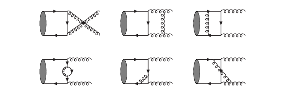
Figure 2: Representative Feynman diagrams for S[1]01→g​g{}^{1}{S}_{0}^{[1]}\rightarrow gg at one-loop level.

At next to leading order in αs\alpha_{s}, there are virtual corrections and real corrections. Fig. 2 corresponds to Feynman diagrams of virtual corrections, where only distinct forms of diagrams are shown. Contribution of these virtual corrections reads

ΓV​(S[1]01→g​g)=CA​αsπΓB(1S0[1]→gg)fϵ{[−1ϵ2+(−116+nf9)1ϵ+136(−44+19π2+(4nf−66)ln(4​mQ2μr2))]+𝐪2mQ2[431ϵ2−427​ϵ(nf−31)+449ln(2)+1324(−4(11+24ln(2))nf+24(33−2nf)ln(mQ2μr2)−267π2+874)]}.\displaystyle\begin{split}\Gamma_{\textrm{V}}({}^{1}{S}_{0}^{[1]}\rightarrow gg)=&\frac{C_{A}\alpha_{s}}{\pi}\Gamma_{\textrm{B}}({}^{1}{S}_{0}^{[1]}\rightarrow gg)f_{\epsilon}\{[-\frac{1}{\epsilon^{2}}+(-\frac{11}{6}+\frac{n_{f}}{9})\frac{1}{\epsilon}\\ &+\>\frac{1}{36}(-44+19\pi^{2}+(4n_{f}-66)\ln(\frac{4m_{Q}^{2}}{\mu_{r}^{2}}))]\\ &+\>\frac{\mathbf{q}^{2}}{m_{Q}^{2}}[\frac{4}{3}\frac{1}{\epsilon^{2}}-\frac{4}{27\epsilon}(n_{f}-31)+\frac{44}{9}\ln(2)\\ &+\>\frac{1}{324}(-4(11+24\ln(2))n_{f}+24(33-2n_{f})\ln(\frac{m_{Q}^{2}}{\mu_{r}^{2}})-267\pi^{2}+874)]\}.\end{split} (25)

While other terms agree with those in Refs.[9, 7], the result of relativistic correction here is new. Feynman diagrams for real corrections are drawn in Fig. 3 and Fig. 4, which correspond to final states with three gluons and q​q¯​gq\overline{q}g respectively. Results for these two sets of real corrections are

Γ⁡(S[1]01→g​g​g)=CA​αsπfϵΓB(1S0[1]→gg){1ϵ2+116​ϵ+18118−2324π2+𝐪2mQ2[−43​ϵ2−4ϵ+754(−139+12π2)]},\displaystyle\begin{split}\Gamma({}^{1}{S}_{0}^{[1]}\rightarrow ggg)=&\ \frac{C_{A}\alpha_{s}}{\pi}f_{\epsilon}\Gamma_{\textrm{B}}({}^{1}{S}_{0}^{[1]}\rightarrow gg)\{\frac{1}{\epsilon^{2}}+\frac{11}{6\epsilon}+\frac{181}{18}-\frac{23}{24}\pi^{2}\\ &+\frac{\mathbf{q}^{2}}{m_{Q}^{2}}[-\frac{4}{3\epsilon^{2}}-\frac{4}{\epsilon}+\frac{7}{54}(-139+12\pi^{2})]\},\end{split} (26a)
Γ⁡(S[1]01→q​q¯​g)=\displaystyle\Gamma({}^{1}{S}_{0}^{[1]}\rightarrow q\overline{q}g)= nf​ΓB​(S[1]01→g​g)​αsπ​fϵΓ⁡(1+ϵ)​Γ​(1−ϵ)​TF​(−23​ϵ−169+𝐪2mQ2​(89​ϵ+10427)).\displaystyle\ n_{f}\Gamma_{\textrm{B}}({}^{1}{S}_{0}^{[1]}\rightarrow gg)\frac{\alpha_{s}}{\pi}\frac{f_{\epsilon}}{\Gamma(1+\epsilon)\Gamma(1-\epsilon)}T_{F}(-\frac{2}{3\epsilon}-\frac{16}{9}+\frac{\mathbf{q}^{2}}{m_{Q}^{2}}(\frac{8}{9\epsilon}+\frac{104}{27})). (26b)

While other terms agree with those in Refs.[9, 7], the results of relativistic corrections here are new. Adding Eqs. (25) and (26), we obtain the NLO QCD corrections plus relativistic corrections for the light hadron decay width of S01{}^{1}{S}_{0} heavy quarkonium

ΓQCDNLO​(S[1]01→LH)\displaystyle\Gamma_{\textrm{QCD}}^{\textrm{NLO}}({}^{1}{S}_{0}^{[1]}\rightarrow\textrm{LH}) =CA​αsπfϵΓB(S0[1]1→gg){1216[−64nf+12(2nf−33)ln(4​mQ2μr2)\displaystyle=\frac{C_{A}\alpha_{s}}{\pi}f_{\epsilon}\Gamma_{\textrm{B}}({}^{1}{S}_{0}^{[1]}\rightarrow gg)\{\frac{1}{216}[-64n_{f}+12(2n_{f}-33)\ln(\frac{4m_{Q}^{2}}{\mu_{r}^{2}})
−93π2+1908]+𝐪2mQ2[1627​ϵ+1324(24(ln(mQ2μr2)+2ln(2))(33−2nf)\displaystyle-93\pi^{2}+1908]+\frac{\mathbf{q}^{2}}{m_{Q}^{2}}[\frac{16}{27\epsilon}+\frac{1}{324}(24(\ln(\frac{m_{Q}^{2}}{\mu_{r}^{2}})+2\ln(2))(33-2n_{f}) (27)
+164nf+237π2−4964)]}.\displaystyle+164n_{f}+237\pi^{2}-4964)]\}.

Adding these terms together, we get the S01{}^{1}{S}_{0} decay width into light hadrons in perturbative QCD

ΓQCD​(S[1]01→LH)=ΓB​(S[1]01→g​g)+ΓBR​(S[1]01→g​g)+ΓQCDNLO​(S[1]01→LH).\Gamma_{\textrm{QCD}}({}^{1}{S}_{0}^{[1]}\rightarrow\textrm{LH})=\Gamma_{\textrm{B}}({}^{1}{S}_{0}^{[1]}\rightarrow gg)+\Gamma_{\textrm{B}}^{\textrm{R}}({}^{1}{S}_{0}^{[1]}\rightarrow gg)+\Gamma_{\textrm{QCD}}^{\textrm{NLO}}({}^{1}{S}_{0}^{[1]}\rightarrow\textrm{LH}). (28)
Refer to caption
Figure 3: Representative Feynman diagrams for S[1]01→g​g​g{}^{1}{S}_{0}^{[1]}\rightarrow ggg.
Refer to caption
Figure 4: Representative Feynman diagrams for S[1]01→q​q¯​g{}^{1}{S}_{0}^{[1]}\rightarrow q\overline{q}g.

IV.2 S[1]01→γ​γ{}^{1}{S}_{0}^{[1]}\rightarrow\gamma\gamma

For QCD corrections to the electromagnetic decay, there is no real correction. Diagrams at Born level and one-loop level are the same as those in Fig. 1 and Fig 2 except that the final state gluons are substituted with photons and diagrams containing three-gluon or four-gluon vertexes are excluded. We then get the results

ΓB​(S[1]01→γ​γ)\displaystyle\Gamma_{\textrm{B}}({}^{1}{S}_{0}^{[1]}\rightarrow\gamma\gamma) =\displaystyle= 12!​12​(2​mQ)​Φ(2​D)​(α​4​π)2​8​eQ4mQ​⟨𝒪⁡(S[1]01)⟩LO,\displaystyle\frac{1}{2!}\frac{1}{2(2m_{Q})}\Phi_{(2D)}(\alpha 4\pi)^{2}\frac{8e_{Q}^{4}}{m_{Q}}\langle\mathcal{O}({}^{1}{S}_{0}^{[1]})\rangle_{\textrm{LO}}, (29a)
ΓBR​(S[1]01→γ​γ)\displaystyle\Gamma_{\textrm{B}}^{\textrm{R}}({}^{1}{S}_{0}^{[1]}\rightarrow\gamma\gamma) =\displaystyle= −43​𝐪2mQ2​ΓB​(S[1]01→γ​γ),\displaystyle-\frac{4}{3}\frac{\mathbf{q}^{2}}{m_{Q}^{2}}\Gamma_{\textrm{B}}({}^{1}{S}_{0}^{[1]}\rightarrow\gamma\gamma), (29b)
ΓV​(S[1]01→γ​γ)\displaystyle\Gamma_{\textrm{V}}({}^{1}{S}_{0}^{[1]}\rightarrow\gamma\gamma) =\displaystyle= ΓB​(S[1]01→γ​γ)​fϵ​αsπ​[π2−203+𝐪2mQ2​(169​ϵ+196−15​π227)],\displaystyle\Gamma_{\textrm{B}}({}^{1}{S}_{0}^{[1]}\rightarrow\gamma\gamma)f_{\epsilon}\frac{\alpha_{s}}{\pi}[\frac{\pi^{2}-20}{3}+\frac{\mathbf{q}^{2}}{m_{Q}^{2}}(\frac{16}{9\epsilon}+\frac{196-15\pi^{2}}{27})], (29c)

where eQe_{Q} is the electric charge of the heavy quark. Results of relativistic corrections in Eq. (29c) are new and the other results agree with those previously calculated as summarized in Ref.[6]. Adding Eqs.(29a), (29b), and (29c), we get the result for the γ​γ\gamma\gamma decay width of S01{}^{1}{S}_{0} heavy quarkonium in perturbative QCD

ΓQCD​(S[1]01→γ​γ)=ΓB​(S[1]01→γ​γ)+ΓBR​(S[1]01→γ​γ)+ΓV​(S[1]01→γ​γ).\Gamma_{\textrm{QCD}}({}^{1}{S}_{0}^{[1]}\rightarrow\gamma\gamma)=\Gamma_{\textrm{B}}({}^{1}{S}_{0}^{[1]}\rightarrow\gamma\gamma)+\Gamma_{\textrm{B}}^{\textrm{R}}({}^{1}{S}_{0}^{[1]}\rightarrow\gamma\gamma)+\Gamma_{\textrm{V}}({}^{1}{S}_{0}^{[1]}\rightarrow\gamma\gamma). (30)

V Perturbative NRQCD Results

Order αs​v2\alpha_{s}v^{2} corrections to the leading order LDME ⟨𝒪0​(S[1]01)⟩\langle\mathcal{O}^{0}({}^{1}{S}_{0}^{[1]})\rangle in perturbative NRQCD have been calculated in Ref.[2], where a cutoff was introduced to regularize the ultraviolet divergences. We rewrite it in dimensional regularization,

⟨𝒪0​(S[1]01)⟩NLO=⟨𝒪0​(S[1]01)⟩LO​[1−4​αs​CF3​π​(μr2μΛ2)ϵ​(1ϵUV−1ϵIR)​𝐪2mQ2].\langle\mathcal{O}^{0}({}^{1}{S}_{0}^{[1]})\rangle_{\textrm{NLO}}=\langle\mathcal{O}^{0}({}^{1}{S}_{0}^{[1]})\rangle_{\textrm{LO}}[1-\frac{4\alpha_{s}C_{F}}{3\pi}(\frac{\mu_{r}^{2}}{\mu_{\Lambda}^{2}})^{\epsilon}(\frac{1}{\epsilon_{\textrm{UV}}}-\frac{1}{\epsilon_{\textrm{IR}}})\frac{\mathbf{q}^{2}}{m_{Q}^{2}}]. (31)

We define the renormalized operator 𝒪R​(S[1]01)\mathcal{O}^{\textrm{R}}({}^{1}{S}_{0}^{[1]}) using the MS¯\overline{\textrm{MS}} scheme

𝒪0​(S[1]01)=ZOMS¯​𝒪R​(S[1]01),\displaystyle\mathcal{O}^{0}({}^{1}{S}_{0}^{[1]})=Z_{O}^{\overline{\textrm{MS}}}\mathcal{O}^{\textrm{R}}({}^{1}{S}_{0}^{[1]}), (32)

where

ZOMS¯=1−4​αs​CF3​π​(μr2μΛ2)ϵ​(1ϵUV+ln⁡4​π−γE)​𝐪2mQ2.\displaystyle Z_{O}^{\overline{\textrm{MS}}}=1-\frac{4\alpha_{s}C_{F}}{3\pi}(\frac{\mu_{r}^{2}}{\mu_{\Lambda}^{2}})^{\epsilon}(\frac{1}{\epsilon_{\textrm{UV}}}+\ln{4\pi}-\gamma_{\textrm{E}})\frac{\mathbf{q}^{2}}{m_{Q}^{2}}. (33)

Therefore

⟨𝒪R​(S[1]01)⟩NLO=[1+4​αs​CF3​π​(μr2μΛ2)ϵ​(1ϵ+ln⁡4​π−γE)​𝐪2mQ2]​⟨𝒪⁡(S[1]01)⟩LO.\displaystyle\langle\mathcal{O}^{\textrm{R}}({}^{1}{S}_{0}^{[1]})\rangle_{\textrm{NLO}}=[1+\frac{4\alpha_{s}C_{F}}{3\pi}(\frac{\mu_{r}^{2}}{\mu_{\Lambda}^{2}})^{\epsilon}(\frac{1}{\epsilon}+\ln{4\pi}-\gamma_{\textrm{E}})\frac{\mathbf{q}^{2}}{m_{Q}^{2}}]\langle\mathcal{O}({}^{1}{S}_{0}^{[1]})\rangle_{\textrm{LO}}. (34)

Considering that

⟨𝒫⁡(S[1]01)⟩LO=𝐪2​⟨𝒪⁡(S[1]01)⟩LO,\displaystyle\langle\mathcal{P}({}^{1}{S}_{0}^{[1]})\rangle_{\textrm{LO}}=\mathbf{q}^{2}\langle\mathcal{O}({}^{1}{S}_{0}^{[1]})\rangle_{\textrm{LO}}, (35)

the decay width into light hadrons in perturbative NRQCD becomes

ΓNRQCD​(S[1]01→LH)=\displaystyle\Gamma_{\textrm{NRQCD}}({}^{1}{S}_{0}^{[1]}\rightarrow\textrm{LH})=
{F(S0[1]1)+𝐪2mQ2[G(S0[1]1)+4​αs​CF3​π(μr2μΛ2)ϵ(1ϵ+ln4π−γE)F(S0[1]1]}⟨𝒪⁡(S[1]01)⟩LOmQ2.\displaystyle\{F({}^{1}{S}_{0}^{[1]})+\frac{\mathbf{q}^{2}}{m_{Q}^{2}}[G({}^{1}{S}_{0}^{[1]})+\frac{4\alpha_{s}C_{F}}{3\pi}(\frac{\mu_{r}^{2}}{\mu_{\Lambda}^{2}})^{\epsilon}(\frac{1}{\epsilon}+\ln{4\pi}-\gamma_{\textrm{E}})F({}^{1}{S}_{0}^{[1]}]\}\frac{\langle\mathcal{O}({}^{1}{S}_{0}^{[1]})\rangle_{\textrm{LO}}}{m_{Q}^{2}}. (36)

The electromagnetic decay rate can be obtained by replacing F⁡(S[1]01)F({}^{1}{S}_{0}^{[1]}) and G⁡(S[1]01)G({}^{1}{S}_{0}^{[1]}) with Fγ​γ​(S[1]01)F_{\gamma\gamma}({}^{1}{S}_{0}^{[1]}) and Gγ​γ​(S[1]01)G_{\gamma\gamma}({}^{1}{S}_{0}^{[1]}) respectively.

VI Matching

Finally we obtain the short distance coefficients by equating results from perturbative QCD in Eqs.(28) and (30) with that from perturbative NRQCD in Eq. (36)

F⁡(S[1]01)=\displaystyle F({}^{1}{S}_{0}^{[1]})= 4​π​αs29​[1+αsπ​−64​nf+12​(2​nf−33)​ln⁡(4​mQ2μr2)−93​π2+190872],\displaystyle\frac{4\pi\alpha_{s}^{2}}{9}[1+\frac{\alpha_{s}}{\pi}\frac{-64n_{f}+12(2n_{f}-33)\ln(\frac{4m_{Q}^{2}}{\mu_{r}^{2}})-93\pi^{2}+1908}{72}], (37a)
G⁡(S[1]01)=\displaystyle G({}^{1}{S}_{0}^{[1]})= 4​π​αs29{−43+αsπ1108[48ln(2)(25−2nf)+164nf−4964\displaystyle\frac{4\pi\alpha_{s}^{2}}{9}\{-\frac{4}{3}+\frac{\alpha_{s}}{\pi}\frac{1}{108}[48\ln(2)(25-2n_{f})+164n_{f}-4964
+24(33−2nf)ln(mQ2μr2)+192ln(μΛ2mQ2)+237π2]},\displaystyle+24(33-2n_{f})\ln(\frac{m_{Q}^{2}}{\mu_{r}^{2}})+192\ln(\frac{\mu_{\Lambda}^{2}}{m_{Q}^{2}})+237\pi^{2}]\}, (37b)
Fγ​γ​(S[1]01)=\displaystyle F_{\gamma\gamma}({}^{1}{S}_{0}^{[1]})= 2​π​α2​eQ4​(1+αsπ​π2−203),\displaystyle 2\pi\alpha^{2}e_{Q}^{4}(1+\frac{\alpha_{s}}{\pi}\frac{\pi^{2}-20}{3}), (37c)
Gγ​γ​(S[1]01)=\displaystyle G_{\gamma\gamma}({}^{1}{S}_{0}^{[1]})= 2​π​α2​eQ4​{−43+αsπ​127​[48​ln⁡(μΛ2mQ2)−96​ln⁡(2)−15​π2+196]},\displaystyle 2\pi\alpha^{2}e_{Q}^{4}\{-\frac{4}{3}+\frac{\alpha_{s}}{\pi}\frac{1}{27}[48\ln(\frac{\mu_{\Lambda}^{2}}{m_{Q}^{2}})-96\ln(2)-15\pi^{2}+196]\}, (37d)

where QCD corrections for G⁡(S[1]01)G({}^{1}{S}_{0}^{[1]}) and Gγ​γ​(S[1]01)G_{\gamma\gamma}({}^{1}{S}_{0}^{[1]}) are new while the other results agree with those in Refs. [9, 2, 7, 6]. With these short distance coefficients, we can update the decay widths of S01{}^{1}{S}_{0} heavy quarkonium into light hadrons and two photons.

VII Phenomenology

The above obtained result can be used in S01{}^{1}{S}_{0} charmonium and bottomonium decays. In the following we will focus on the ηc\eta_{c} decay width into light hadrons (approximately the total width) and decay width into two photons. In these decays there are two unknown LDMEs. In principle, one can fix these LDMEs either through direct fit with experimental data[30] or calculation from lattice QCD[17, 18]. The order v2v^{2} LDME is ultraviolet divergent and needs to be regularized [20]. For lattice calculations this is performed by imposing a hard cut-off regulator. However, due to slow convergence of this regularization, the results available from lattice calculations of order v2v^{2} LDME suffer from large uncertainties[17, 18]. On the other hand, we find that direct fit of the two LDMEs using experimental measurements of γ​γ\gamma\gamma width and total width of ηc\eta_{c} can not give reliable values due to the approximate linear dependence of the two theoretical predictions for these two decays.

Therefore we determine the two LDMEs using the potential model method recently introduced in Refs.[19, 20, 21]. A widely accepted potential model, the Cornell potential[31]

V⁡(r)=−κr+σ​r,V(r)=-\frac{\kappa}{r}+\sigma r, (38)

is chosen in this work. Since the spin dependent effect is not included in this potential, the LDMEs calculated this way are accurate up to corrections of relative order v2v^{2}. However, as argued in Ref. [20], this error is in fact much less than the order v2v^{2} (about 30%30\%), thus we attach an uncertainty of 30%30\% to the central value of the order v2v^{2} LDMEs to account for the error due to this static potential approximation.

In solving the Schrödinger equation [32], there are three unknown parameters. σ=0.1682±0.0053​GeV2\sigma=0.1682\pm 0.0053~\textrm{GeV}^{2} is taken from the average of lattice calculations[20] and the mass parameter is expressed in terms of the 1​S1S-2​S2S mass splitting[19, 20]. Here we take m⁡(ψ⁡(2​S))−m⁡(J/ψ)=589.188±0.028​MeVm(\psi(2S))-m(J/\psi)=589.188\pm 0.028\ \textrm{MeV} [33]. The last remaining parameter is fixed by equating theoretical predictions to experimentally measured results. When we use the decay width formula, we resum a class of relativistic corrections at leading order in αs\alpha_{s} for γ​γ\gamma\gamma decay as in Refs.[20, 21]. For the experimental input, we make use of this approximation ΓLH​(ηc​(n​S))=Γtotal​(ηc​(n​S))\Gamma^{\textrm{LH}}(\eta_{c}(nS))=\Gamma^{\textrm{total}}(\eta_{c}(nS)). For ηc\eta_{c}, we use Γγ​γ​(ηc)\Gamma^{\gamma\gamma}(\eta_{c}) (or ΓLH​(ηc)\Gamma^{\textrm{LH}}(\eta_{c})) as input to obtain one set LDMEs which are then utilized to obtain ΓLH​(ηc)\Gamma^{\textrm{LH}}(\eta_{c}) (or Γγ​γ​(ηc)\Gamma^{\gamma\gamma}(\eta_{c})). For ηc​(2​S)\eta_{c}(2S), we use the total width as input and make predictions for the γ​γ\gamma\gamma decay width. We take mcm_{c} to be 1.4±0.2​GeV1.4\pm 0.2\ \textrm{GeV} [20], α=1/137\alpha=1/137, ΛQCD=0.39​GeV\Lambda_{\textrm{QCD}}=0.39\ \textrm{GeV} and vary the renormalization scale μr\mu_{r} and NRQCD factorization scale μΛ\mu_{\Lambda} separately from 1​GeV1\ \textrm{GeV} to 3​GeV3\ \textrm{GeV} with 2​GeV2\ \textrm{GeV} as the central value. The LDMEs are expressed in terms of the wave function at the origin |ℛ⁡(0)|2|\mathcal{R}(0)|^{2} and ⟨𝒗2⟩\langle\bm{v}^{2}\rangle as defined in Eqs. (13) and (15). In each determination of these LDMEs and the corresponding decay width, we evaluate the variations caused by the uncertainties of the parameters and summarize them in the tables. Because the potential does not take into account of the spin effects, we attach each v2v^{2} LDME an uncertainty ⟨𝒗2⟩\langle\bm{v}^{2}\rangle of 30%30\% of the central value. In each case, various uncertainties are added in quadrature to give the total uncertainty.

For ηc\eta_{c}, with the γ​γ\gamma\gamma width Γγ​γ​(ηc)=7.2±0.7±2.0​KeV\Gamma^{\gamma\gamma}(\eta_{c})=7.2\pm 0.7\pm 2.0\ \textrm{KeV} [33] as input, the determined LDMEs are

|ℛηcγ​γ​(0)|2\displaystyle|\mathcal{R}_{\eta_{c}}^{\gamma\gamma}(0)|^{2} =\displaystyle= 0.881−0.313+0.382​GeV3,\displaystyle 0.881^{+0.382}_{-0.313}\ \textrm{GeV}^{3}, (39a)
⟨𝒗2⟩ηcγ​γ\displaystyle\langle\bm{v}^{2}\rangle_{\eta_{c}}^{\gamma\gamma} =\displaystyle= 0.228−0.100+0.126,\displaystyle 0.228^{+0.126}_{-0.100}, (39b)

where the superscript γ​γ\gamma\gamma indicates that we use the γ​γ\gamma\gamma decay width as input. Various uncertainties are summarized in Table 1. The most significant uncertainty comes from the experimental data. At order αs​v2\alpha_{s}v^{2}, another dependence on NRQCD factorization scale μΛ\mu_{\Lambda} is introduced. However, as we can see from Table 1, variations of LDMEs are small when we change μΛ\mu_{\Lambda} from 1​GeV1\ \textrm{GeV} to 3​GeV3\ \textrm{GeV}. In Fig. 5, we present μr\mu_{r} dependence of three sets of LDMEs in terms of |ℛηc​(0)|2|\mathcal{R}_{\eta_{c}}(0)|^{2} and ⟨𝒗2⟩ηc\langle\bm{v}^{2}\rangle_{\eta_{c}}, where the other parameters are fixed to their central values. Of these three sets of lines, LO represents calculation without any QCD corrections, NLO∗\textrm{NLO}^{*} corresponds to that including QCD corrections but only for terms at leading order in vv, and NLO means our new result with order αs​v2\alpha_{s}v^{2} correction taken into account. The LDMEs corresponding to NLO∗\textrm{NLO}^{*} have been computed earlier in Ref. [20] and can be compared here with the values including the new order αs​v2\alpha_{s}v^{2} corrections. We can see from this figure that these two lines are close to each other, which reflects the fact that the effect of the new order αs​v2\alpha_{s}v^{2} correction is not large.

Refer to caption
(a) μr\mu_{r} dependence of |ℛηcγ​γ​(0)|2|\mathcal{R}_{\eta_{c}}^{\gamma\gamma}(0)|^{2}
Refer to caption
(b) μr\mu_{r} dependence of ⟨𝒗2⟩ηcγ​γ\langle\bm{v}^{2}\rangle_{\eta_{c}}^{\gamma\gamma}
Figure 5: μr\mu_{r} dependence of LDMEs for ηc\eta_{c} using the observed γ​γ\gamma\gamma width as input. LO represents values without QCD corrections, NLO∗\textrm{NLO}^{*} includes QCD corrections only for terms at leading order in vv, and NLO takes into account our new QCD corrections to order v2v^{2} terms.
Table 1: LDMEs obtained from potential model for ηc\eta_{c} and the predicted total width of ηc\eta_{c}, the superscript γ​γ\gamma\gamma indicates that the observed width of ηc→γ​γ\eta_{c}\rightarrow\gamma\gamma is used as input. The second row gives central values while the followed rows give variations with respect to related parameters.
Case |ℛηcγ​γ​(0)|2​(GeV3)|\mathcal{R}_{\eta_{c}}^{\gamma\gamma}(0)|^{2}\ (\textrm{GeV}^{3}) ⟨𝒗2⟩ηcγ​γ\langle\bm{v}^{2}\rangle_{\eta_{c}}^{\gamma\gamma} Γtotal​(ηc)​(MeV)\Gamma^{\textrm{total}}(\eta_{c})\ (\textrm{MeV})
central 0.881 0.228 31.4
+Δ​⟨𝒗2⟩ηc+\Delta\langle\bm{v}^{2}\rangle_{\eta_{c}} 0.078 0.068 -3.5
−Δ​⟨𝒗2⟩ηc-\Delta\langle\bm{v}^{2}\rangle_{\eta_{c}} -0.075 -0.068 2.6
+Δ​mc+\Delta m_{c} 0.187 -0.065 0.3
−Δ​mc-\Delta m_{c} -0.167 0.102 -3.4
+Δ​σ+\Delta\sigma 0.022 0.020 -0.9
−Δ​σ-\Delta\sigma -0.021 -0.019 0.8
+Δ​μr+\Delta\mu_{r} -0.059 0.005 -9.2
−Δ​μr-\Delta\mu_{r} 0.217 -0.018 27.3
+Δ​μΛ+\Delta\mu_{\Lambda} -0.036 0.003 -0.6
−Δ​μΛ-\Delta\mu_{\Lambda} 0.064 -0.005 1.1
+Δ​Γηc+\Delta\Gamma_{\eta_{c}} 0.232 -0.019 10.3
−Δ​Γηc-\Delta\Gamma_{\eta_{c}} -0.243 0.021 -9.9
Refer to caption
(a) μr\mu_{r} dependence of |ℛηcLH​(0)|2|\mathcal{R}_{\eta_{c}}^{\textrm{LH}}(0)|^{2}
Refer to caption
(b) μr\mu_{r} dependence of ⟨𝒗2⟩ηcLH\langle\bm{v}^{2}\rangle_{\eta_{c}}^{\textrm{LH}}
Figure 6: μr\mu_{r} dependence of LDMEs for ηc\eta_{c} using the observed total width as input. LO represents values without QCD corrections, NLO∗\textrm{NLO}^{*} includes QCD corrections only for terms at leading order in vv, and NLO takes into account our new QCD corrections to order v2v^{2} terms.

Utilizing this set of LDMEs as input, we get the total decay width for ηc\eta_{c}

Γtotal​(ηc)=31.4−14.4+29.3​MeV.\Gamma^{\textrm{total}}(\eta_{c})=31.4^{+29.3}_{-14.4}\ \textrm{MeV}. (40)

This value is in consistency with experimental measurement 28.6±2.2​MeV28.6\pm 2.2\ \textrm{MeV} [33], although there are large uncertainties. The details of the uncertainties are summarized in Table 1. Here, the uncertainty induced by the μr\mu_{r} dependence predominates over that from the experimental input of the γ​γ\gamma\gamma width of ηc\eta_{c}.

Table 2: LDMEs obtained from potential model for ηc\eta_{c} and the predicted γ​γ\gamma\gamma width of ηc\eta_{c}, where the superscript LH indicates that the observed total width of ηc\eta_{c} is used as input. The second row gives the central values while the followed rows give variations with respect to related parameters.
Case |ℛηcLH​(0)|2​(GeV3)|\mathcal{R}_{\eta_{c}}^{\textrm{LH}}(0)|^{2}\ (\textrm{GeV}^{3}) ⟨𝒗2⟩ηcLH\langle\bm{v}^{2}\rangle_{\eta_{c}}^{\textrm{LH}} Γ⁡(ηc→γ​γ)​(KeV)\Gamma(\eta_{c}\rightarrow\gamma\gamma)\ (\textrm{KeV})
central 0.814 0.234 6.61
+Δ​⟨𝒗2⟩ηc+\Delta\langle\bm{v}^{2}\rangle_{\eta_{c}} 0.194 0.070 0.90
−Δ​⟨𝒗2⟩ηc-\Delta\langle\bm{v}^{2}\rangle_{\eta_{c}} -0.131 -0.070 -0.54
+Δ​mc+\Delta m_{c} 0.163 -0.065 -0.07
−Δ​mc-\Delta m_{c} -0.090 0.095 0.71
+Δ​σ+\Delta\sigma 0.042 0.018 0.19
−Δ​σ-\Delta\sigma -0.038 -0.018 -0.16
+Δ​μr+\Delta\mu_{r} 0.201 -0.017 2.47
−Δ​μr-\Delta\mu_{r} -0.189 0.016 -2.73
+Δ​μΛ+\Delta\mu_{\Lambda} -0.020 0.002 0.13
−Δ​μΛ-\Delta\mu_{\Lambda} 0.036 -0.003 -0.21
+Δ​Γηc+\Delta\Gamma_{\eta_{c}} 0.052 -0.004 0.46
−Δ​Γηc-\Delta\Gamma_{\eta_{c}} -0.053 0.005 -0.47

If, on the other hand, we use the total width of ηc\eta_{c}, Γtotal​(ηc)=28.6±2.2​MeV\Gamma^{\textrm{total}}(\eta_{c})=28.6\pm 2.2\ \textrm{MeV} [33] as input, then we get another set of LDMEs

|ℛηcLH​(0)|2\displaystyle|\mathcal{R}_{\eta_{c}}^{\textrm{LH}}(0)|^{2} =\displaystyle= 0.814−0.256+0.332​GeV3,\displaystyle 0.814^{+0.332}_{-0.256}\ \textrm{GeV}^{3}, (41a)
⟨𝒗2⟩ηcLH\displaystyle\langle\bm{v}^{2}\rangle_{\eta_{c}}^{\textrm{LH}} =\displaystyle= 0.234−0.099+0.121,\displaystyle 0.234^{+0.121}_{-0.099}, (41b)

where the superscript LH indicates that we use the total width of ηc\eta_{c} as input. Variations with respect to the parameters are summarized in Table 2. The experimental uncertainty in this case is small and the main uncertainty comes from the relatively strong μr\mu_{r} dependence of the theoretical prediction. The μr\mu_{r} dependence of the two LDMEs is shown in Fig. 6. As in previous case, we display another two sets of LDMEs, where only QCD corrections at leading order in vv are taken into account or no QCD correction is considered. The two sets with QCD corrections show great improvement of μr\mu_{r} dependence with respect to the one without QCD corrections, and they are almost parallel to each other. The only difference between the two sets of values is that the αs​v2\alpha_{s}v^{2} correction enhances |ℛηc​(0)|2|\mathcal{R}_{\eta_{c}}(0)|^{2} by about 30%30\%. This enhanced LDME coincides with previously obtained value using Γγ​γ​(ηc)\Gamma^{\gamma\gamma}(\eta_{c}) as input. The value of ⟨𝒗2⟩ηc\langle\bm{v}^{2}\rangle_{\eta_{c}} is relatively stable. With this set of LDMEs, we obtain the γ​γ\gamma\gamma decay width

Γγ​γ​(ηc)=6.61−2.83+2.77​KeV,\Gamma^{\gamma\gamma}(\eta_{c})=6.61^{+2.77}_{-2.83}\ \textrm{KeV}, (42)

which is also consistent with the experimental measurement 7.2±0.7±2.0​KeV7.2\pm 0.7\pm 2.0\ \textrm{KeV} [33].

Since now we have two sets of values for the two LDMEs for ηc\eta_{c} in Eqs.(39) and (41), we can combine these values to get a better estimation. The uncertaintes in Table 1 and Table 2 are correlated, and we use the method in Ref. [20] to treat these correlations. First we construct a two-by-two covariance matrix for ⟨𝒪⁡(S[1]01)⟩ηcγ​γ\langle\mathcal{O}({}^{1}{S}_{0}^{[1]})\rangle_{\eta_{c}}^{\gamma\gamma} and ⟨𝒪⁡(S[1]01)⟩ηcLH\langle\mathcal{O}({}^{1}{S}_{0}^{[1]})\rangle_{\eta_{c}}^{\textrm{LH}}. It describes correlations between the variations in the two tables and is defined as Cj​k=∑iΔj​i​Δk​iC_{jk}=\sum_{i}\Delta_{ji}\Delta_{ki} with Δj​i=12​(Oj​i+−Oj​i−)\Delta_{ji}=\frac{1}{2}(O_{ji}^{+}-O_{ji}^{-}). The indexes j,kj,k refer to these two leading order LDMEs and ii runs through every item in Table 1 and Table 2. Oj​i+O_{ji}^{+} and Oj​i−O_{ji}^{-} correspond to the plus and minus variations of the LDMEs. For the ii-th item in Table 1 or Table 2, we define the χi2\chi^{2}_{i} as

χi2=∑j,k(Oj​i−O¯i)​(C−1)j​k​(Ok​i−O¯i)\displaystyle\chi^{2}_{i}=\sum_{j,k}(O_{ji}-\overline{O}_{i})(C^{-1})_{jk}(O_{ki}-\overline{O}_{i}) (43)

and minimize it to get the average value O¯i\overline{O}_{i} for ⟨𝒪(S0[1]1)ηc\langle\mathcal{O}({}^{1}{S}_{0}^{[1]})_{\eta_{c}}. Once we obtain the values of ⟨𝒪(S0[1]1)ηc\langle\mathcal{O}({}^{1}{S}_{0}^{[1]})_{\eta_{c}}, we use the potential model to get the values of ⟨𝒫(S0[1]1)ηc\langle\mathcal{P}({}^{1}{S}_{0}^{[1]})_{\eta_{c}}. We perform this calculation for each of the items in Table 1 and Table 2 , treat the renormalization scale μr\mu_{r} and NRQCD factorization scale μΛ\mu_{\Lambda} simply as the same quantities in the two tables and express the results in terms of |ℛηc​(0)||\mathcal{R}_{\eta_{c}}(0)| and ⟨𝒗2⟩ηc\langle\bm{v}^{2}\rangle_{\eta_{c}}. The results are

|ℛηc​(0)|2\displaystyle|\mathcal{R}_{\eta_{c}}(0)|^{2} =\displaystyle= 0.834−0.197+0.281​GeV3,\displaystyle 0.834^{+0.281}_{-0.197}\ \textrm{GeV}^{3}, (44a)
⟨𝒗2⟩ηc\displaystyle\langle\bm{v}^{2}\rangle_{\eta_{c}} =\displaystyle= 0.232−0.098+0.121,\displaystyle 0.232^{+0.121}_{-0.098}, (44b)

with the details of the uncertainties given in Table 3. We note that the uncertainties here for |ℛηc​(0)|2|\mathcal{R}_{\eta_{c}}(0)|^{2} are smaller than those in Eqs.(39) and (41) .

Table 3: The averages of the LDMEs for ηc\eta_{c}. The second row gives the central values and subsequent rows give variations with respect to various uncertainties.
Case |ℛηc​(0)|2​(GeV3)|\mathcal{R}_{\eta_{c}}(0)|^{2}\ (\textrm{GeV}^{3}) ⟨𝒗2⟩ηc\langle\bm{v}^{2}\rangle_{\eta_{c}}
central 0.834 0.232
+Δ​⟨𝒗2⟩ηc+\Delta\langle\bm{v}^{2}\rangle_{\eta_{c}} 0.159 0.070
−Δ​⟨𝒗2⟩ηc-\Delta\langle\bm{v}^{2}\rangle_{\eta_{c}} -0.115 -0.070
+Δ​mc+\Delta m_{c} 0.170 -0.065
−Δ​mc-\Delta m_{c} -0.113 0.097
+Δ​σ+\Delta\sigma 0.036 0.019
−Δ​σ-\Delta\sigma -0.033 -0.018
+Δ​μr+\Delta\mu_{r} 0.124 -0.010
−Δ​μr-\Delta\mu_{r} -0.069 0.006
+Δ​μΛ+\Delta\mu_{\Lambda} -0.025 0.002
−Δ​μΛ-\Delta\mu_{\Lambda} 0.044 -0.004
+Δ​Γηcγ​γ+\Delta\Gamma_{\eta_{c}}^{\gamma\gamma} 0.069 -0.006
−Δ​Γηcγ​γ-\Delta\Gamma_{\eta_{c}}^{\gamma\gamma} -0.072 0.006
+Δ​Γηct​o​t​a​l+\Delta\Gamma_{\eta_{c}}^{total} 0.037 -0.003
−Δ​Γηct​o​t​a​l-\Delta\Gamma_{\eta_{c}}^{total} -0.037 0.003

For ηc​(2​S)\eta_{c}(2S), we use the observed total width 14±7​Mev14\pm 7\ \textrm{Mev}[33] as input and get the LDMEs for ηc​(2​S)\eta_{c}(2S)

|ℛηc​(2​S)LH​(0)|2\displaystyle|\mathcal{R}_{\eta_{c}(2S)}^{\textrm{LH}}(0)|^{2} =\displaystyle= 0.423−0.230+0.245​GeV3,\displaystyle 0.423^{+0.245}_{-0.230}\ \textrm{GeV}^{3}, (45a)
⟨𝒗2⟩ηc​(2​S)LH\displaystyle\langle\bm{v}^{2}\rangle_{\eta_{c}(2S)}^{\textrm{LH}} =\displaystyle= 0.255−0.109+0.130.\displaystyle 0.255^{+0.130}_{-0.109}. (45b)

Some potential model calculations of the squared wave function at the origin in Ref.[34] give 0.418 for the logarithmic potential[35], 0.529 for the QCD-motivated B-T model[36], and 0.559 for the power-law potential[37]. Our result is consistent with their values. Table 4 gives details with various uncertainties. In the ηc​(2​S)\eta_{c}(2S) case, both the μr\mu_{r} dependence of theoretical result and the experimental input of the total width have large uncertainties and therefore the LDMEs are subject to relatively large uncertainties. In Fig. 7, we present μr\mu_{r} dependence of this set of LDMEs. The shape of the lines is similar to Fig. 6 except the value for |ℛηc​(2​S)​(0)|2|\mathcal{R}_{\eta_{c}(2S)}(0)|^{2} here is smaller by about a factor of 2.

Table 4: LDMEs obtained from potential model for ηc​(2​S)\eta_{c}(2S) and the predicted γ​γ\gamma\gamma width of ηc​(2​S)\eta_{c}(2S), where the superscript LH indicates that the total width of ηc​(2​S)\eta_{c}(2S) is used as input. The second row gives the central values while the followed rows give variations with respect to related parameters.
Case |ℛηcLH​(0)|2​(GeV3)|\mathcal{R}_{\eta_{c}}^{\textrm{LH}}(0)|^{2}\ (\textrm{GeV}^{3}) ⟨𝒗2⟩ηcLH\langle\bm{v}^{2}\rangle_{\eta_{c}}^{\textrm{LH}} Γ⁡(ηc​(2​S)→γ​γ)​(KeV)\Gamma(\eta_{c}(2S)\rightarrow\gamma\gamma)\ (\textrm{KeV})
central 0.423 0.255 3.34
+Δ​⟨𝒗2⟩ηc​(2​S)+\Delta\langle\bm{v}^{2}\rangle_{\eta_{c}(2S)} 0.121 0.076 0.58
−Δ​⟨𝒗2⟩ηc​(2​S)-\Delta\langle\bm{v}^{2}\rangle_{\eta_{c}(2S)} -0.077 -0.076 -0.33
+Δ​mc+\Delta m_{c} 0.077 -0.069 -0.08
−Δ​mc-\Delta m_{c} -0.035 0.099 0.47
+Δ​σ+\Delta\sigma 0.024 0.019 0.11
−Δ​σ-\Delta\sigma -0.022 -0.019 -0.10
+Δ​μr+\Delta\mu_{r} 0.102 -0.016 1.22
−Δ​μr-\Delta\mu_{r} -0.091 0.014 -1.33
+Δ​μΛ+\Delta\mu_{\Lambda} -0.012 0.002 0.07
−Δ​μΛ-\Delta\mu_{\Lambda} 0.022 -0.003 -0.11
+Δ​Γηc​(2​S)+\Delta\Gamma_{\eta_{c}(2S)} 0.167 -0.026 1.47
−Δ​Γηc​(2​S)-\Delta\Gamma_{\eta_{c}(2S)} -0.192 0.029 -1.58
Refer to caption
(a) μr\mu_{r} dependence of |ℛηc​(2​S)LH​(0)|2|\mathcal{R}_{\eta_{c}(2S)}^{\textrm{LH}}(0)|^{2}
Refer to caption
(b) μr\mu_{r} dependence of ⟨𝒗2⟩ηc​(2​S)LH\langle\bm{v}^{2}\rangle_{\eta_{c}(2S)}^{\textrm{LH}}
Figure 7: μr\mu_{r} dependence of LDMEs for ηc​(2​S)\eta_{c}(2S) using the total width as input. LO represents values without QCD corrections, NLO∗\textrm{NLO}^{*} includes QCD corrections only for terms at leading order in vv, and NLO takes into account our new QCD corrections to order v2v^{2} terms.

Exploiting this set of LDMEs, we can make predictions for the γ​γ\gamma\gamma decay width of ηc​(2​S)\eta_{c}(2S),

Γγ​γ​(ηc​(2​S))=3.34−2.10+2.06​KeV.\Gamma^{\gamma\gamma}(\eta_{c}(2S))=3.34^{+2.06}_{-2.10}\ \textrm{KeV}. (46)

This prediction is consistent with the experimental observation that the branching fraction of γ​γ\gamma\gamma decay is smaller than 5×10−45\times 10^{-4} [33]. Another experiment measured Γγ​γ​(ηc​(2​S))​B​(ηc​(2​S)→K​K¯​π)=(0.18±0.05±0.02)​Γγ​γ​(ηc​(1​S))​B​(ηc​(1​S)→K​K¯​π)\Gamma_{\gamma\gamma}(\eta_{c}(2S))B(\eta_{c}(2S)\rightarrow K\overline{K}\pi)=(0.18\pm 0.05\pm 0.02)\Gamma_{\gamma\gamma}(\eta_{c}(1S))B(\eta_{c}(1S)\rightarrow K\overline{K}\pi) [38] and assumed that the branching fractions of ηc\eta_{c} and ηc​(2​S)\eta_{c}(2S) decays into KS​K​πK_{S}K\pi were equal, and made use of Γ⁡(ηc→γ​γ)=7.4±0.4±2.3​KeV\Gamma(\eta_{c}\rightarrow\gamma\gamma)=7.4\pm 0.4\pm 2.3\ \textrm{KeV}, and then derived Γ⁡(ηc​(2​S))=1.3±0.6​KeV\Gamma(\eta_{c}(2S))=1.3\pm 0.6\ \textrm{KeV}[33, 38]. Our result is not in contradiction with their measurement within errors.

VIII Summary

Within the framework of NRQCD, we calculate order αs​v2\alpha_{s}v^{2} corrections to decays of S01{}^{1}{S}_{0} heavy quarkonium into light hadrons and two photons. In both processes, infrared divergences are found to be canceled through the matching of perturbative QCD and perturbative NRQCD results. There are two unknown NRQCD LDMEs, which are determined using potential model method[19, 20, 21] either with the observed total width or two photon width as input. When using Γγ​γ​(ηc)\Gamma^{\gamma\gamma}(\eta_{c}) as input, we get |ℛηcγ​γ​(0)|2=0.881−0.313+0.382​GeV3|\mathcal{R}_{\eta_{c}}^{\gamma\gamma}(0)|^{2}=0.881^{+0.382}_{-0.313}\ \textrm{GeV}^{3} and ⟨𝒗2⟩ηcγ​γ=0.228−0.100+0.126\langle\bm{v}^{2}\rangle_{\eta_{c}}^{\gamma\gamma}=0.228^{+0.126}_{-0.100}, from which we predict Γtotal​(ηc)=31.4−14.4+29.3​MeV\Gamma^{\textrm{total}}(\eta_{c})=31.4^{+29.3}_{-14.4}\ \textrm{MeV}. Alternatively, when using Γtotal​(ηc)\Gamma^{\textrm{total}}(\eta_{c}) as input, we get |ℛηcLH​(0)|2=0.814−0.256+0.332​GeV3|\mathcal{R}_{\eta_{c}}^{\textrm{LH}}(0)|^{2}=0.814^{+0.332}_{-0.256}\ \textrm{GeV}^{3} and ⟨𝒗2⟩ηcLH=0.234−0.099+0.121\langle\bm{v}^{2}\rangle_{\eta_{c}}^{\textrm{LH}}=0.234^{+0.121}_{-0.099}, and we predict the γ​γ\gamma\gamma width of ηc\eta_{c} to be Γγ​γ​(ηc)=6.61−2.83+2.77​KeV\Gamma^{\gamma\gamma}(\eta_{c})=6.61^{+2.77}_{-2.83}\ \textrm{KeV}. All these predictions agree well with experimental data. We then combine these two kinds of determination of LDMEs and get the average values |ℛηc​(0)|2=0.834−0.197+0.281​GeV3|\mathcal{R}_{\eta_{c}}(0)|^{2}=0.834^{+0.281}_{-0.197}\ \textrm{GeV}^{3} and ⟨𝒗2⟩ηc=0.232−0.098+0.121\langle\bm{v}^{2}\rangle_{\eta_{c}}=0.232^{+0.121}_{-0.098}. For ηc​(2​S)\eta_{c}(2S), we use the observed total width as input and find |ℛηc​(2​S)LH​(0)|2=0.423−0.230+0.245​GeV3|\mathcal{R}_{\eta_{c}(2S)}^{\textrm{LH}}(0)|^{2}=0.423^{+0.245}_{-0.230}\ \textrm{GeV}^{3} and ⟨𝒗2⟩ηc​(2​S)LH=0.255−0.109+0.130\langle\bm{v}^{2}\rangle_{\eta_{c}(2S)}^{\textrm{LH}}=0.255^{+0.130}_{-0.109}. With this set of LDMEs, we predict the γ​γ\gamma\gamma width of ηc​(2​S)\eta_{c}(2S) to be 3.34−2.10+2.06​KeV3.34^{+2.06}_{-2.10}\ \textrm{KeV}, which is not in contradiction with data within uncertainties. Consequently, the order αs​v2\alpha_{s}v^{2} corrections (especially the one to the decay into light hadrons) are found to have significant effects on improving the consistency between theoretical predictions and experimental measurements.

N​o​t​e​a​d​d​e​dNote\ added. When we finished the calculations and are preparing this paper, a related work appears[39] that also gives αs​v2\alpha_{s}v^{2} corrections to the γ​γ\gamma\gamma decay width. We find our results for this channel agree with theirs, while we have also calculated the light hadron decay width.

Acknowledgement

We thank G. T. Bodwin, Y. Fan, and C. Meng for helpful discussions. We also thank Franz F. Schöberl for providing us with schroedinger.nb to solve the Schrödinger equation. This work was supported by the National Natural Science Foundation of China (No.11021092, No.11075002) and the Ministry of Science and Technology of China (No.2009CB825200).

References