跳到论文正文
W Papers独立论文阅读器 arXiv:1104.2985 论文正文 计算阅读时间 · 0%
引用这篇论文根据当前论文元数据生成,正式投稿前建议核对。


License: arXiv.org perpetual non-exclusive license
arXiv:1104.2985v2 [math.AP] 20 Apr 2011
11footnotetext: Dipartimento di Matematica, Università degli studi di Brescia, Italia. rinaldo@ing.unibs.it22footnotetext: Di.S.T.A., Università del Piemonte Orientale, Italia, mauro.garavello@mfn.unipmn.it33footnotetext: Université d’Orléans, UFR Sciences, Bâtiment de mathématiques - Rue de Chartres B.P. 6759 - 45067 Orléans cedex 2, France, magali.lecureux-mercier@univ-orleans.fr

A Class of Non-Local Models for Pedestrian Traffic

Rinaldo M. Colombo    Mauro Garavello    Magali Lécureux-Mercier
Abstract

We present a new class of macroscopic models for pedestrian flows. Each individual is assumed to move towards a fixed target, deviating from the best path according to the instantaneous crowd distribution. The resulting equation is a conservation law with a nonlocal flux. Each equation in this class generates a Lipschitz semigroup of solutions and is stable with respect to the functions and parameters defining it. Moreover, key qualitative properties such as the boundedness of the crowd density are proved. Specific models are presented and their qualitative properties are shown through numerical integrations.

2000 Mathematics Subject Classification: 35L65, 90B20.

Keywords: Crowd Dynamics, Macroscopic Pedestrian Model, Non-Local Conservation Laws.

1 Introduction

From a macroscopic point of view, a moving crowd is described by its density ρ=ρ⁡(t,x)\rho=\rho(t,x), so that for any subset AA of the plane, the quantity ∫Aρ⁡(t,x)​d​x\int_{A}\rho(t,x)\mathinner{\mathrm{d}{x}} is the total number of individuals in AA at time tt. In standard situations, the number of individuals is constant, so that conservation laws of the type ∂tρ+divx​(ρ​𝐯)=0\partial_{t}\rho+\mathinner{\rm div}_{x}(\rho\,{\mathbf{v}})=0 are the natural tool for the description of crowd dynamics. A key issue is the choice of the speed 𝐯\mathbf{v}, which should describe not only the target of the pedestrians and the modulus of their speed, but also their attitude to adapt their path choice to the crowd density they estimate to find along this path.

Our starting point is the following Cauchy problem for the conservation law

{∂tρ+div⁡(ρ​v​(ρ)​(ν⁡(x)+ℐ⁡(ρ)))=0,ρ⁡(0,x)=ρ0​(x).\left\{\begin{array}[]{l}\partial_{t}\rho+\mathinner{\rm div}\left(\rho\,v(\rho)\,\left(\nu(x)+\mathcal{I}(\rho)\right)\right)=0\,,\\ \rho(0,x)=\rho_{0}(x)\,.\end{array}\right. (1.1)

The scalar function ρ↦v⁡(ρ)\rho\mapsto v(\rho) describes the modulus of the pedestrians’ speed, independently from geometrical considerations. In other words, an individual at time tt and position x∈ℝNx\in{\mathbb{R}}^{N} moves at the speed v⁡(ρ⁡(t,x))v\left(\rho(t,x)\right) that depends on the density ρ⁡(t,x)\rho(t,x) evaluated at the same time tt and position xx. Given that the density is ρ\rho, the vector ν⁡(x)+ℐ⁡(ρ)\nu(x)+\mathcal{I}(\rho) describes the direction that the individual located at xx follows and has norm (approximately) 11. More precisely, the individual at position xx and time tt is assumed to move in the direction ν⁡(x)+(ℐ⁡(ρ⁡(t)))​(x)\nu(x)+\left(\mathcal{I}\left(\rho(t)\right)\right)(x).

In situations like the evacuation of a closed space Ω⊂ℝN\Omega\subset{\mathbb{R}}^{N}, it is natural to assume that the first choice of each pedestrian is to follow a path optimal with respect to the visible geometry, for instance the geodesic. As soon as walls or obstacles are relevant, it is necessary to take into consideration the discomfort felt by pedestrians walking along walls or too near to corners, see for instance [19, 21] and the references therein.

The vector (ℐ​(ρ​(t)))​(x)\left(\mathcal{I}\left(\rho(t)\right)\right)(x) describes the deviation from the direction ν⁡(x)\nu(x) due to the density distribution ρ⁡(t)\rho(t) at time tt. Hence, the operator ℐ\mathcal{I} is in general nonlocal, so that (ℐ​(ρ​(t)))​(x)\left(\mathcal{I}\left(\rho(t)\right)\right)(x) depends on all the values of the density ρ⁡(t)\rho(t) at time tt in a neighborhood of xx. More formally, it depends on all the function ρ⁡(t)∈𝐋1​(ℝN,[0,R])\rho(t)\in{\mathbf{L}^{1}}({\mathbb{R}}^{N};[0,R]) and not only on the value ρ⁡(t,x)∈[0,R]\rho(t,x)\in[0,R]. The case in which ℐ=0\mathcal{I}=0 is equivalent to assume that the paths followed by the individuals are chosen a priori, independently from the dynamics of the crowd.

Here we present two specific choices that fit in (1.1). A first criterion assumes that each individual aims at avoiding high crowd densities. Fix a mollifier η\eta. Then, the convolution (ρ∗η)(\rho*\eta) is an average of the crowd density around xx. This leads to the natural choice

ℐ⁡(ρ)=−ε​∇(ρ∗η)1+‖∇(ρ∗η)‖2,\mathcal{I}(\rho)=-\varepsilon\,\frac{\nabla(\rho*\eta)}{\sqrt{1+{\left\|\nabla(\rho*\eta)\right\|}^{2}}}\,, (1.2)

related to [4], which states that individuals deviate from the optimal path trying to avoid entering regions with higher densities. Through numerical integrations, below we provide examples of solutions to (1.1)–(1.2). They show the interesting phenomenon of pattern formation. In the case of a crowd walking along a corridor, coherently with the experimental observation described in the literature, see for instance [17, 18, 20, 28], the solution to (1.1)–(1.2) self-organizes into lanes. The width of these lanes depends on the size of the support of the averaging kernel η\eta. This feature is stable with respect to strong variations in the initial datum and also in the geometry. Indeed, we have lane formation also in the case of the evacuation of a room, when the crowd density sharply increases in front of the door. Section 4.1 is devoted to this property.

From the analytical point of view, we note that the convolution term in (1.2) seems not sufficient to regularize solutions. Indeed, the present analytical framework is devised to consider solutions in 𝐋1∩𝐁𝐕{\mathbf{L}^{1}}\cap\mathbf{BV}. Both in the case of a crush in front of an exit (Section 4.2) and in the specific example in Section 4.3, numerical simulations highlight that the space gradient of ρ\rho increases dramatically.

According to (1.2), pedestrians evaluate the crowd density all around their position. When restrictions on the angle of vision are relevant, the following choice is reasonable:

ℐ⁡(ρ)=−ε​∇∫ℝNρ(y)η(x−y)φ((y−x)⋅g(x))d​y1+‖∇∫ℝNρ(y)η(x−y)φ((y−x)⋅g(x))d​y‖2.\mathcal{I}(\rho)=-\varepsilon\,\frac{\nabla\,\int_{{\mathbb{R}}^{N}}\rho(y)\,\eta(x-y)\,\varphi\!\left((y-x)\cdot g(x)\right)\mathinner{\mathrm{d}{y}}}{\sqrt{1+{\left\|\nabla\,\int_{{\mathbb{R}}^{N}}\rho(y)\,\eta(x-y)\,\varphi\!\left((y-x)\cdot g(x)\right)\mathinner{\mathrm{d}{y}}\right\|}^{2}}}\,. (1.3)

Here, η\eta is a fixed mollifier as above and the smooth function φ\varphi weights the deviation from the preferred direction g⁡(x)g(x).

We note that the constructions in [22, 23] and [14] fit in the present setting. Indeed, there the following choices were considered:

{∂tρ−div(ρf2(ρ)∇φ)=0|∇φ|=1/f⁡(ρ) and {∂tρ−div(ρf2(ρ)∇φ)=0−ε​Δ​φ+|∇φ|2=1/(f⁡(ρ)+ε)2.\left\{\begin{array}[]{l}\partial_{t}\rho-\mathinner{\rm div}\left(\rho\,f^{2}(\rho)\,\nabla\varphi\right)=0\\ {\left|\nabla\varphi\right|}=1/f(\rho)\end{array}\right.\hskip 20.00003pt\mbox{ and }\hskip 20.00003pt\left\{\begin{array}[]{l}\partial_{t}\rho-\mathinner{\rm div}\left(\rho\,f^{2}(\rho)\,\nabla\varphi\right)=0\\ -\varepsilon\Delta\varphi+{\left|\nabla\varphi\right|}^{2}=1/\left(f(\rho)+\varepsilon\right)^{2}\,.\end{array}\right.

The former admits an immediate interpretation: the direction ∇φ\nabla\varphi of the speed 𝐯\mathbf{v} is chosen along the solutions to the eikonal equations, i.e. all pedestrians follow the shortest path, weighing at every instant the length of paths with the amount of people that are moving along it. In the former case, ν⁡(x)=0\nu(x)=0 and ℐ⁡(ρ)\mathcal{I}(\rho) is the gradient of the solution to the eikonal equation with 1/f⁡(ρ)1/f(\rho) in the right hand side, while in the latter case ν⁡(x)=0\nu(x)=0 and ℐ⁡(ρ)\mathcal{I}(\rho) is the gradient of the solution to an elliptic partial differential equation.

The model introduced in [13, 29] relies on this measure valued conservation law:

∂tμ+div⁡(μ​v)=0 where v=ν⁡(x)+∫ℝ2f⁡(|x−y|)​φ​((y−x)⋅ν⁡(x))​x−y‖x−y‖​d​μt​(y).\partial_{t}\mu+\mathinner{\rm div}(\mu\,v)=0\hskip 10.00002pt\mbox{ where }\hskip 10.00002ptv=\nu(x)+\int_{{\mathbb{R}}^{2}}f({\left|x-y\right|})\,\varphi\left((y-x)\cdot\nu(x)\right)\frac{x-y}{{\left\|x-y\right\|}}\mathinner{\mathrm{d}{\mu}}_{t}(y)\,.

Here the unknown is a map μ:[0,T]→ℳ⁡(ℝN,ℝ)\mu\colon[0,T]\to\mathcal{M}({\mathbb{R}}^{N};{\mathbb{R}}) assigning at every time tt a positive measure μ⁡(t)\mu(t) which substitutes the crowd density, in the sense that the amount of people that at time tt are in AA is (μ​(t))​(A)\left(\mu(t)\right)(A). Contrary to this model, the present framework is the space of 𝐋1{\mathbf{L}^{1}} densities and physical a priori 𝐋∞{\mathbf{L}^{\infty}} bounds on the solutions to (1.1) are rigorously proved, preventing any focusing effect as well as the rise of any Dirac delta. Moreover, below we prove global in time existence of solutions, their continuous dependence from the initial data and their stability with respect to variations in the speed law 𝐯\mathbf{v}.

In [12], the geometric part ν\nu of the speed is chosen a priori, while its modulus depend on the density as well as on the gradient of the density:

∂tρ+div⁡(ρ​φ​(ρ,∇ρ)​ν​(x))=0.\partial_{t}\rho+\mathinner{\rm div}\left(\rho\,\varphi(\rho,\nabla\rho)\,\nu(x)\right)=0\,.

On the contrary, the model introduced in [7] postulates a nonlocal dependence of the speed from the density:

∂tρ+div⁡(ρ​v​(ρ∗η)​ν​(x))=0,\partial_{t}\rho+\mathinner{\rm div}\left(\rho\,v(\rho*\eta)\,\nu(x)\right)=0\,,

which amounts to assume that pedestrians choose their behavior according to evaluations of an average of the density around their position, rather than according to the density at their place. The following second order model was presented in [1, 16] and does not fit in (1.1):

{∂tρ+div⁡(ρ​v)=0∂tv+(v⋅∇)v=F(ρ,∇ρ,v),\left\{\begin{array}[]{l}\partial_{t}\rho+\mathinner{\rm div}(\rho v)=0\\ \partial_{t}v+(v\cdot\nabla)v=F(\rho,\nabla\rho,v)\,,\end{array}\right.

we refer to the review [2] for further details. To underline the variety of analytical techniques with which crowd dynamics has been tackled, we recall the further approaches: optimal transport in [5], the mean field limit in [15], the functional analytic one in [26, 27] and the nonclassical shocks used in [6, 10, 11].

Throughout this work, we set all statements in all ℝN{\mathbb{R}}^{N}. In Section 3 we show how the present framework is able to take into consideration the presence of various constraints. In the case of pedestrian dynamics, for instance, this amounts to prove that no individual passes through the walls of a given room, provided the initial datum is assigned inside it. Concerning the dimension, our main applications are referred to the case of crowd dynamics, i.e. N=2N=2. Nevertheless, from the analytical point of view, considering the case of a general NN does not add any difficulty. Furthermore, we believe that the present setting can be reasonably applied also to, say, fishes and birds moving in ℝ3{\mathbb{R}}^{3}, for example in predator-prey like situations as described in [8].

The next section is devoted to the analytical properties of (1.1): well posedness and stability. The general theory is particularized to specific examples in Section 3, where the presence of obstacle (walls) is considered. Sample numerical integrations are provided in Section 4. The final Section 5 collects the analytical proofs. We defer to Appendix A further remarks related to the geometry of the physical domain.

2 Analytical Results

In the following, N∈ℕ∖{0}N\in{\mathbb{N}}\setminus\{0\} is the (fixed) space dimension. We denote ℝ+=[0,+∞[{\mathbb{R}}^{+}=\left[0,+\infty\right[\,; the open ball in ℝN{\mathbb{R}}^{N} centered at xx and with radius r>0r>0 is B⁡(x,r)B(x,r) and we let WN=∫0π/2(cos⁡ϑ)N​d​ϑW_{N}=\int_{0}^{\pi/2}(\cos\vartheta)^{N}\,\mathinner{\mathrm{d}{\vartheta}}. As usual, we denote SN−1={x∈ℝN:‖x‖=1}S^{N-1}=\left\{x\in{\mathbb{R}}^{N}\colon{\left\|x\right\|}=1\right\}.

The density ρ\rho can be defined as the fraction of space occupied by pedestrians, so that ρ\rho turns out to be a nondimensional scalar in [0,1][0,1]. Otherwise, it can be useful to think at ρ\rho as measured in, say, individuals/m2\mbox{individuals}/m^{2} and varying in [0,R][0,R], with R>0R>0 being a given maximal density, for example R=8​individuals/m2R=8\;\mbox{individuals}/m^{2}.

Our first step in the study of (1.1) is the formal definition of solution.

Definition 2.1.

Fix a positive TT and an initial datum ρ0∈𝐋1​(ℝN,[0,R])\rho_{0}\in{\mathbf{L}^{1}}({\mathbb{R}}^{N};[0,R]). A function ρ∈𝐂0​([0,T],𝐋1​(ℝN,ℝ))\rho\in\mathbf{C}^{0}\left([0,T];{\mathbf{L}^{1}}({\mathbb{R}}^{N};{\mathbb{R}})\right) is a weak entropy solution to (1.1) if it is a Kružkov solution to the Cauchy problem for the scalar conservation law

{∂tρ+div⁡(ρ​v​(ρ)​w​(t,x))=0ρ⁡(0,x)=ρ0​(x)\left\{\begin{array}[]{l}\partial_{t}\rho+\mathinner{\rm div}\left(\rho\,v(\rho)\,w(t,x)\right)=0\\ \rho(0,x)=\rho_{0}(x)\end{array}\right. (2.1)

where w⁡(t,x)=ν⁡(x)+(ℐ⁡(ρ⁡(t)))​(x)w(t,x)=\nu(x)+\left(\mathcal{I}\left(\rho(t)\right)\right)(x).

In other words, recalling [24, Definition 1], for all k∈ℝk\in{\mathbb{R}}, for all φ∈𝐂c∞(]−∞,T]×ℝN;ℝ+)\varphi\in\mathbf{C}_{c}^{\infty}(\left]-\infty,T\right]\times{\mathbb{R}}^{N};{\mathbb{R}}^{+}),

∫0T∫ℝN[|ρ−k|​∂tφ+[(ρ​v​(ρ)−k​v​(k))​w​(t,x)⋅∇φ−k​v​(k)​div​w​(t,x)​φ]​sgn(ρ−k)]​d​x​d​t\displaystyle\int_{0}^{T}\!\!\!\int_{{\mathbb{R}}^{N}}\!\left[{\left|\rho-k\right|}\,\partial_{t}\varphi+\left[\left(\rho\,v(\rho)-k\,v(k)\right)\,w(t,x)\cdot\nabla\varphi-k\,v(k)\mathinner{\rm div}w(t,x)\,\varphi\right]\mathop{\rm sgn}(\rho-k)\right]\mathinner{\mathrm{d}{x}}\mathinner{\mathrm{d}{t}}
+∫ℝN|ρ0(x)−k|φ(0,x)d​x⩾0.\displaystyle+\int_{{\mathbb{R}}^{N}}{\left|\rho_{0}(x)-k\right|}\,\varphi(0,x)\mathinner{\mathrm{d}{x}}\geqslant 0.

On the functions defining the general model (1.1), we introduce the following hypotheses:

(v)

v∈𝐂2​(ℝ,ℝ)v\in\mathbf{C}^{2}\left({\mathbb{R}};{\mathbb{R}}\right) is non increasing, v⁡(0)=Vv(0)=V and v⁡(R)=0v(R)=0 for fixed V,R>0V,R>0.

(ν\boldsymbol{\nu})

ν∈(𝐂2∩𝐖1,∞)​(ℝN,ℝN)\nu\in(\mathbf{C}^{2}\cap{\mathbf{W}^{1,\infty}})({\mathbb{R}}^{N};{\mathbb{R}}^{N}) is such that div​ν∈(𝐖1,1∩𝐖1,∞)​(ℝN,ℝ)\mathinner{\rm div}\nu\in({\mathbf{W}^{1,1}}\cap{\mathbf{W}^{1,\infty}})({\mathbb{R}}^{N};{\mathbb{R}}).

(I)

ℐ∈𝐂0​(𝐋1​(ℝN,[0,R]),𝐂2​(ℝN,ℝN))\mathcal{I}\in\mathbf{C}^{0}\left({\mathbf{L}^{1}}({\mathbb{R}}^{N};[0,R]);\mathbf{C}^{2}({\mathbb{R}}^{N};{\mathbb{R}}^{N})\right) satisfies the following estimates:

  1. (I.1)

    There exists an increasing CI∈𝐋l​o​c∞​(ℝ+,ℝ+)C_{I}\in{\mathbf{L}_{loc}^{\infty}}({\mathbb{R}^{+}};{\mathbb{R}^{+}}) such that, for all r∈𝐋1​(ℝN,[0,R])r\in{\mathbf{L}^{1}}({\mathbb{R}}^{N};[0,R]),

    ‖ℐ⁡(r)‖𝐖1,∞⩽CI​(‖r‖𝐋1) and ‖div​ℐ​(r)‖𝐋1⩽CI​(‖r‖𝐋1).\displaystyle{\left\|\mathcal{I}(r)\right\|}_{{\mathbf{W}^{1,\infty}}}\leqslant C_{I}({\left\|r\right\|}_{{\mathbf{L}^{1}}})\hskip 10.00002pt\mbox{ and }\hskip 10.00002pt{\left\|\mathcal{\mathinner{\rm div}I}(r)\right\|}_{{\mathbf{L}^{1}}}\leqslant C_{I}({\left\|r\right\|}_{{\mathbf{L}^{1}}})\,.
  2. (I.2)

    There exists an increasing CI∈𝐋l​o​c∞​(ℝ+,ℝ+)C_{I}\in{\mathbf{L}_{loc}^{\infty}}({\mathbb{R}^{+}};{\mathbb{R}^{+}}) such that, for all r∈𝐋1​(ℝN,[0,R])r\in{\mathbf{L}^{1}}({\mathbb{R}}^{N};[0,R]),

    ‖∇divℐ(r)‖𝐋1⩽CI(‖r‖𝐋1).{\left\|\nabla\mathinner{\rm div}\mathcal{I}(r)\right\|}_{{\mathbf{L}^{1}}}\leqslant C_{I}({\left\|r\right\|}_{{\mathbf{L}^{1}}})\,.
  3. (I.3)

    There exists a constant KIK_{I} such that for all r1,r2∈𝐋1​(ℝN,[0,R])r_{1},r_{2}\in{\mathbf{L}^{1}}({\mathbb{R}}^{N};[0,R]),

    ‖ℐ⁡(r1)−ℐ⁡(r2)‖𝐋∞\displaystyle{\left\|\mathcal{I}(r_{1})-\mathcal{I}(r_{2})\right\|}_{{\mathbf{L}^{\infty}}} ⩽\displaystyle\leqslant KI⋅‖r1−r2‖𝐋1,\displaystyle K_{I}\cdot{\left\|r_{1}-r_{2}\right\|}_{{\mathbf{L}^{1}}}\,,
    ‖ℐ⁡(r1)−ℐ⁡(r2)‖𝐋1+‖div⁡(ℐ⁡(r1)−ℐ⁡(r2))‖𝐋1\displaystyle{\left\|\mathcal{I}(r_{1})-\mathcal{I}(r_{2})\right\|}_{{\mathbf{L}^{1}}}+{\left\|\mathinner{\rm div}(\mathcal{I}(r_{1})-\mathcal{I}(r_{2}))\right\|}_{{\mathbf{L}^{1}}} ⩽\displaystyle\leqslant KI⋅‖r1−r2‖𝐋1.\displaystyle K_{I}\cdot{\left\|r_{1}-r_{2}\right\|}_{{\mathbf{L}^{1}}}\,.

Furthermore, throughout we denote by qq the map q:[0,R]↦ℝq\colon[0,R]\mapsto{\mathbb{R}} defined by q⁡(ρ)=ρ​v​(ρ)q(\rho)=\rho\,v(\rho).

As a first justification of these conditions, note that they make Definition 2.1 acceptable.

Lemma 2.2.

Fix a positive TT. Let (v), (𝛎\boldsymbol{\nu}) and (I.1) hold. Choose an arbitrary density r∈𝐂0​([0,T],𝐋1​(ℝN,[0,R]))r\in\mathbf{C}^{0}\left([0,T];{\mathbf{L}^{1}}({\mathbb{R}}^{N};[0,R])\right). Then, the Cauchy problem

{∂tρ+div⁡(ρ​v​(ρ)​w​(t,x))=0ρ⁡(0,x)=ρ0​(x) with w⁡(t,x)=ν⁡(x)+(ℐ⁡(r⁡(t)))​(x)\left\{\begin{array}[]{l}\partial_{t}\rho+\mathinner{\rm div}\left(\rho\,v(\rho)\,w(t,x)\right)=0\\ \rho(0,x)=\rho_{0}(x)\end{array}\right.\hskip 20.00003pt\mbox{ with }\hskip 20.00003ptw(t,x)=\nu(x)+\left(\mathcal{I}\left(r(t)\right)\right)(x) (2.2)

satisfies the assumptions of Kružkov Theorem [24, Theorem 5].

This lemma is proved in Section 5 below. In Section 3 we show that the above assumption (I) allows to comprehend physically reasonable cases.

The next result is devoted to the proof of existence and uniqueness for (1.1). It is obtained through Banach Fixed Point Theorem.

Theorem 2.3.

Let (v), (𝛎\boldsymbol{\nu}) and (I) hold. Choose any ρ0∈(𝐋1∩𝐁𝐕)​(ℝN,[0,R])\rho_{0}\in({\mathbf{L}^{1}}\cap\mathbf{BV})({\mathbb{R}}^{N};[0,R]). Then, there exists a unique weak entropy solution ρ∈𝐂0​(ℝ+,𝐋1​(ℝN,[0,R]))\rho\in\mathbf{C}^{0}\left({\mathbb{R}^{+}};{\mathbf{L}^{1}}({\mathbb{R}}^{N};[0,R])\right) to (1.1). Moreover, ρ\rho satisfies the bounds

‖ρ⁡(t)‖𝐋1\displaystyle{\left\|\rho(t)\right\|}_{{\mathbf{L}^{1}}} =\displaystyle= ‖ρ0‖𝐋1, for a.e. ​t∈ℝ+,\displaystyle{\left\|\rho_{0}\right\|}_{{\mathbf{L}^{1}}}\,,\mbox{ for a.e. }t\in{\mathbb{R}^{+}}\,,
TV⁡(ρ⁡(t))\displaystyle\mathinner{\rm TV}(\rho(t)) ⩽\displaystyle\leqslant TV(ρ0)ek​t+tek​tNWN‖q‖𝐋∞​([0,R])(‖∇divν‖𝐋1+CI(‖ρ0‖𝐋1)),\displaystyle\mathinner{\rm TV}(\rho_{0})\,e^{kt}+te^{kt}NW_{N}{\left\|q\right\|}_{{\mathbf{L}^{\infty}}([0,R])}\left({\left\|\nabla\mathinner{\rm div}\nu\right\|}_{{\mathbf{L}^{1}}}+C_{I}({\left\|\rho_{0}\right\|}_{{\mathbf{L}^{1}}})\right)\,,

where k=(2​N+1)​‖q′‖𝐋∞​([0,R])​(‖∇ν‖𝐋∞+CI​(‖ρ0‖𝐋1))k=(2N+1){\left\|q^{\prime}\right\|}_{{\mathbf{L}^{\infty}}([0,R])}\left({\left\|\nabla\nu\right\|}_{{\mathbf{L}^{\infty}}}+C_{I}({\left\|\rho_{0}\right\|}_{{\mathbf{L}^{1}}})\right).

Using the techniques in [7, 9], we now obtain the continuous dependence of the solution to (1.1) from the initial datum and its stability with respect to vv, ν\nu and ℐ\mathcal{I} in the natural norms.

Theorem 2.4.

Let (v), (𝛎\boldsymbol{\nu}) and (I) be satisfied by both systems

{∂tρ+div⁡[ρ​v1​(ρ)​(ν1​(x)+ℐ1​(ρ))]=0ρ⁡(0,x)=ρ0,1​(x) and {∂tρ+div⁡[ρ​v2​(ρ)​(ν2​(x)+ℐ2​(ρ))]=0ρ⁡(0,x)=ρ0,2​(x)\left\{\begin{array}[]{@{}l@{}}\partial_{t}\rho+\mathinner{\rm div}\left[\rho\,v_{1}(\rho)\,\left(\nu_{1}(x)+\mathcal{I}_{1}(\rho)\right)\right]=0\\ \rho(0,x)=\rho_{0,1}(x)\end{array}\right.\hskip 10.00002pt\mbox{ and }\hskip 10.00002pt\left\{\begin{array}[]{@{}l@{}}\partial_{t}\rho+\mathinner{\rm div}\left[\rho\,v_{2}(\rho)\,\left(\nu_{2}(x)+\mathcal{I}_{2}(\rho)\right)\right]=0\\ \rho(0,x)=\rho_{0,2}(x)\end{array}\right.

with ρ0,1,ρ0,2∈(𝐋1∩𝐁𝐕)​(ℝN,[0,R])\rho_{0,1},\rho_{0,2}\in({\mathbf{L}^{1}}\cap\mathbf{BV})({\mathbb{R}}^{N};[0,R]). Then, the two solutions ρ1\rho_{1} and ρ2\rho_{2} satisfy

‖ρ1​(t)−ρ2​(t)‖𝐋1\displaystyle{\left\|\rho_{1}(t)-\rho_{2}(t)\right\|}_{{\mathbf{L}^{1}}} ⩽\displaystyle\leqslant C⁡(t)​(‖ρ0,1−ρ0,2‖𝐋1+‖q1−q2‖𝐖1,∞CLOSE\displaystyle C(t)\big({\left\|\rho_{0,1}-\rho_{0,2}\right\|}_{{\mathbf{L}^{1}}}+{\left\|q_{1}-q_{2}\right\|}_{{\mathbf{W}^{1,\infty}}}
OPEN+‖ν1−ν2‖𝐋∞+‖div⁡(ν1−ν2)‖𝐋1+d⁡(ℐ1,ℐ2))\displaystyle\hskip 20.00003pt\hskip 10.00002pt+{\left\|\nu_{1}-\nu_{2}\right\|}_{{\mathbf{L}^{\infty}}}+{\left\|\mathinner{\rm div}(\nu_{1}-\nu_{2})\right\|}_{{\mathbf{L}^{1}}}+d\left(\mathcal{I}_{1},\mathcal{I}_{2}\right)\big)

where d⁡(ℐ1,ℐ2)=sup{‖ℐ1​(ρ)−ℐ2​(ρ)‖𝐋∞+‖div​ℐ1​(ρ)−div​ℐ2​(ρ)‖𝐋1:ρ∈𝐋1​(ℝN,[0,R])}\displaystyle d(\mathcal{I}_{1},\mathcal{I}_{2})=\sup\left\{{\left\|\mathcal{I}_{1}(\rho)-\mathcal{I}_{2}(\rho)\right\|}_{{\mathbf{L}^{\infty}}}+{\left\|\mathinner{\rm div}\mathcal{I}_{1}(\rho)-\mathinner{\rm div}\mathcal{I}_{2}(\rho)\right\|}_{{\mathbf{L}^{1}}}\colon\rho\in{\mathbf{L}^{1}}({\mathbb{R}}^{N};[0,R])\right\}, the map C∈𝐂0​(ℝ+,ℝ+)C\in\mathbf{C}^{0}({\mathbb{R}}^{+};{\mathbb{R}}^{+}) vanishes at t=0t=0 and depends on TV⁡(ρ0,1)\mathinner{\rm TV}(\rho_{0,1}), ‖ρ0,1‖𝐋1{\left\|\rho_{0,1}\right\|}_{{\mathbf{L}^{1}}}, ‖ν1‖𝐋∞{\left\|\nu_{1}\right\|}_{{\mathbf{L}^{\infty}}}, ‖div​ν1‖𝐖1,1{\left\|\mathinner{\rm div}\nu_{1}\right\|}_{{\mathbf{W}^{1,1}}}, ‖q1‖𝐖1,∞{\left\|q_{1}\right\|}_{{\mathbf{W}^{1,\infty}}}, ‖q2‖𝐖1,∞{\left\|q_{2}\right\|}_{{\mathbf{W}^{1,\infty}}}.

Thanks to these stability results, several control problems can be proved to admit a solution through a direct application of Weierstraß Theorem. A possible standard application could be the minimization of the evacuation time from a given room. Describing the actions of a controller able to determine the initial pedestrians’ distribution and/or their preferred paths, one is lead to an optimal control problem with the initial datum ρ0\rho_{0} and the vector field ν\nu as control parameters, for instance. Without any loss of generality, the compact sets on which the optimization is made can be {ρ∈(𝐋1∩𝐁𝐕)​(ℝN,[0,1]):TV⁡(ρ)<M}\left\{\rho\in({\mathbf{L}^{1}}\cap\mathbf{BV})({\mathbb{R}}^{N};[0,1])\colon\mathinner{\rm TV}(\rho)<M\right\} for ρ0\rho_{0} and {ν∈𝐂2​(ℝN,B⁡(0,1)¯):‖∇3ν‖⩽M}\left\{\nu\in\mathbf{C}^{2}\left({\mathbb{R}}^{N};\overline{B(0,1)}\right)\colon{\left\|\nabla^{3}\nu\right\|}\leqslant M\right\} for ν\nu, where M>0M>0 is arbitrary.

A different problem solved by the same analytical techniques is that of the dynamic parameter estimation. Once real data are available, one is left with the problem of determining the various parameters entering ν\nu, vv or ℐ\mathcal{I}. Theorem 2.4 ensures the existence of the parameters that allows a best agreement between the solutions to (1.1) and the data.

3 The Models

This section is devoted to the study of specific cases of (1.1). Aiming at real applications, it is necessary to take into consideration the various constraints that are present on the movement of pedestrians. Therefore, we introduce the subset Ω\Omega of ℝN{\mathbb{R}}^{N} which characterizes the region reachable to any individual. The boundary ∂Ω\partial\Omega consists of walls that can not be crossed by any individual. On the set Ω\Omega we require that

(𝛀\boldsymbol{\Omega})

Ω⊆ℝN\Omega\subseteq{\mathbb{R}}^{N} is the closure of a non empty connected open set. If ∂Ω\partial\Omega is not empty, there exists a positive rΩr_{\Omega} such that the function

d∂Ω:B⁡(∂Ω,rΩ)∩Ω→ℝ+x↦inf{d⁡(x,w):w∈∂Ω}\begin{array}[]{ccccc}d_{\partial\Omega}&\colon&B(\partial\Omega,r_{\Omega})\cap\Omega&\to&{\mathbb{R}}^{+}\\ &&x&\mapsto&\inf\left\{d(x,w)\colon w\in\partial\Omega\right\}\end{array}

is of class 𝐂2​(B⁡(∂Ω,rΩ)∩Ω,ℝ+)\mathbf{C}^{2}\left(B(\partial\Omega,r_{\Omega})\cap\Omega;{\mathbb{R}}^{+}\right).

Note that we do not require Ω\Omega to be bounded. This assumptions allows us to introduce the inward normal

n​(x)=∇d∂Ω​(x)n(x)=\nabla d_{\partial\Omega}(x) (3.1)

on all the strip B⁡(∂Ω,rΩ)∩ΩB(\partial\Omega,r_{\Omega})\cap\Omega. Moreover, ‖n⁡(x)‖=1{\left\|n(x)\right\|}=1.

For the present models to be acceptable, it is mandatory that no individual enters any wall, provided the initial datum is supported inside the physically admissible space. Analytically, this is described by the following invariance property:

(P) The model (1.1) is invariant with respect to Ω\Omega if

sptρ0⊂Ω⟹sptρ⁡(t)⊂Ω​ for all ​t⩾0.\mathop{\rm spt}\rho_{0}\subset\Omega\hskip 20.00003pt\hskip 20.00003pt\Longrightarrow\hskip 20.00003pt\hskip 20.00003pt\mathop{\rm spt}\rho(t)\subset\Omega\mbox{ for all }t\geqslant 0\,.

Below, we show that theorems 2.3 and 2.4 can be applied to reasonable crowd dynamics models, in the sense that the presence of a physically admissible set Ω\Omega is also considered and its invariance in the sense of (P) is proved. More precisely, we show below the following sufficient condition for invariance.

Proposition 3.1.

Let ν\nu, ℐ\mathcal{I} and Ω\Omega satisfy (𝛎\boldsymbol{\nu}), (𝐈\boldsymbol{I}) and (Ω\boldsymbol{\Omega}). If for all x∈∂Ωx\in\partial\Omega and ρ∈𝐋1​(ℝN,[0,R])\rho\in{\mathbf{L}^{1}}({\mathbb{R}}^{N};[0,R]) with sptρ⊆Ω\mathop{\rm spt}\rho\subseteq\Omega

(ν⁡(x)+(ℐ⁡(ρ))​(x))⋅n⁡(x)⩾0\left(\nu(x)+\left(\mathcal{I}(\rho)\right)(x)\right)\cdot n(x)\geqslant 0 (3.2)

then, property (P) holds.

3.1 The Model (1.1)–(1.2)

The starting point for (1.1)–(1.2) is provided by the degenerate parabolic model

∂tρ+div⁡(ρ​v​(ρ)​(ν⁡(x)−ε​∇ψ​(ρ)1+‖∇ψ​(ρ)‖2))=0\partial_{t}\rho+\mathinner{\rm div}\left(\rho\,v(\rho)\bigg(\nu(x)-\varepsilon\frac{\nabla\psi(\rho)}{\sqrt{1+{\left\|\nabla\psi(\rho)\right\|}^{2}}}\bigg)\right)=0

introduced in [4], which fits in (1.1) with ℐ(ρ)=−ε∇ψ(ρ)/1+‖∇ψ​(ρ)‖2\mathcal{I}(\rho)=-\varepsilon\,\nabla\psi(\rho)\,\left/\sqrt{1+{\left\|\nabla\psi(\rho)\right\|}^{2}}\right., motivated by the desire of each individual to avoid entering regions occupied by a high crowd density. Here, ψ\psi is a suitable weight function. Assuming that each pedestrian reacts to evaluations of averages of the density, we obtain

∂tρ+div⁡(ρ​v​(ρ)​(ν⁡(x)−ε​∇(ψ⁡(ρ)∗η)1+‖∇(ψ⁡(ρ)∗η)‖2))=0.\partial_{t}\rho+\mathinner{\rm div}\left(\rho\,v(\rho)\bigg(\nu(x)-\varepsilon\frac{\nabla(\psi(\rho)*\eta)}{\sqrt{1+{\left\|\nabla(\psi(\rho)*\eta)\right\|}^{2}}}\bigg)\right)=0\,.

Here, we avoid the introduction of ψ\psi to limit the analytical technicalities, obtaining (1.1)–(1.2). We assume throughout that ε>0\varepsilon>0 is fixed and that the mollifier η\eta satisfies

(η\boldsymbol{\eta})

η∈𝐂c3​(ℝN,ℝ+)\eta\in\mathbf{C}_{c}^{3}({\mathbb{R}}^{N};{\mathbb{R}}^{+}) with ∫ℝNη⁡(x)​d​x=1\int_{{\mathbb{R}}^{N}}\eta(x)\mathinner{\mathrm{d}{x}}=1.

This convolution kernel has a key role: the individual at xx deviates from the optimal path considering the crowd present in the region x−sptηx-\mathop{\rm spt}\eta, when no walls are present. The value η⁡(ξ)\eta(\xi) is the relevance that the individual at xx gives to the density ρ⁡(x−ξ)\rho(x-\xi) located at x−ξx-\xi.

The next result shows that the present model fits in the framework described in Section 2 when applied on all of ℝN{\mathbb{R}}^{N}.

Lemma 3.2.

Fix ε>0\varepsilon>0 and let η\eta satisfy (𝛈\boldsymbol{\eta}). Then, the operator ℐ\mathcal{I} in (1.2) satisfies (I).

When the region Ω\Omega reachable by the crowd is restricted by the walls ∂Ω\partial\Omega, we intend the convolution restricted to Ω\Omega

(ρ∗η)​(x)=∫Ωρ⁡(y)​η​(y−x)​d​y(\rho*\eta)(x)=\int_{\Omega}\rho(y)\,\eta(y-x)\,\mathinner{\mathrm{d}{y}} (3.3)

which coincide with the previous definition in the case sptρ⊂Ω\mathop{\rm spt}\rho\subset\Omega. A better choice is described in (A.1). The vector ν\nu is here chosen as a sum

ν=g+δ.\nu=g+\delta\,. (3.4)

The former vector gg is tangent to the “optimal” path, depending only on the geometry of the environment and coherent with it. Hence we assume that

(g)

g∈𝐂2​(ℝN,SN−1)g\in\mathbf{C}^{2}({\mathbb{R}}^{N};S^{N-1}) satisfies ∇g∈𝐋∞​(ℝN,ℝN×N)\nabla g\in{\mathbf{L}^{\infty}}({\mathbb{R}}^{N};{\mathbb{R}}^{N\times N}), div​g∈(𝐖1,1∩𝐖1,∞)​(ℝN,ℝ)\mathinner{\rm div}g\in({\mathbf{W}^{1,1}}\cap{\mathbf{W}^{1,\infty}})({\mathbb{R}}^{N};{\mathbb{R}}) and the invariance condition g⁡(x)⋅n⁡(x)⩾0g(x)\cdot n(x)\geqslant 0 holds for all x∈∂Ωx\in\partial\Omega.

The latter vector δ\delta describes the discomfort felt when passing too near to walls or obstacles. Below, we choose

δ⁡(x)=λ​α​(x)​n​(x).\delta(x)=\lambda\,\alpha(x)\,n(x)\,. (3.5)

Here, λ∈ℝ+\lambda\in{\mathbb{R}}^{+} is a suitable constant and n⁡(x)n(x) is the inward normal (3.1). The role of the function α\alpha is to confine this discomfort to the region near the walls, i.e. we require

(α\boldsymbol{\alpha})

α∈𝐂2​(ℝN,[0,1])\alpha\in\mathbf{C}^{2}({\mathbb{R}}^{N};[0,1]) is such that α⁡(x)=0\alpha(x)=0 whenever B⁡(x,rΩ)⊆ΩB(x,r_{\Omega})\subseteq\Omega and α⁡(x)=1\alpha(x)=1 for x∈∂Ωx\in\partial\Omega.

A better choice for the discomfort is discussed in Appendix A.

The present setting (1.1)–(1.2) can be effectively applied also in presence of walls, as shown by the next result.

Proposition 3.3.

Let ε>0\varepsilon>0, (v), (Ω\boldsymbol{\Omega}), (𝛈\boldsymbol{\eta}), (g) and (𝛂\boldsymbol{\alpha}) hold. Define ν\nu by (3.4), δ\delta by (3.5) and ℐ\mathcal{I} by (1.2). Assume moreover that either ∂Ω\partial\Omega is compact, or α∈(𝐖2,1∩𝐖2,∞)\alpha\in({\mathbf{W}^{2,1}}\cap{\mathbf{W}^{2,\infty}}) and d∂Ω∈(𝐖3,1∩𝐖3,∞)d_{\partial\Omega}\in({\mathbf{W}^{3,1}}\cap{\mathbf{W}^{3,\infty}}). Then, (1.1)–(1.2) satisfies the assumptions of Theorem 2.3 and Theorem 2.4. Furthermore, if λ⩾ε​R​‖∇η‖𝐋1\lambda\geqslant\varepsilon\,R\,{\left\|\nabla\eta\right\|}_{{\mathbf{L}^{1}}}, then property (P) holds.

3.2 The Model (1.1)–(1.3)

In the framework of (1.1), we now extend the model [13, (2.1)–(2.4)] to take into account the effects of crowd density on the speed modulus, i.e. of v⁡(ρ)v(\rho). Moreover, we interpret the nonlocal term as a weighted average of the density, where the amount of crowd in the direction of the optimal path gg is given more importance.

Using the same notation as above, we thus consider the model (1.1) with

ℐ⁡(ρ)=−ε​∇∫ℝNρ(y)η(x−y)φ((y−x)⋅g(x))d​y1+‖∇∫ℝNρ(y)η(x−y)φ((y−x)⋅g(x))d​y‖2.\mathcal{I}(\rho)=-\varepsilon\,\frac{\nabla\!\!\int_{{\mathbb{R}}^{N}}\rho(y)\,\eta(x-y)\,\varphi\!\left((y-x)\cdot g(x)\right)\mathinner{\mathrm{d}{y}}}{\sqrt{1+{\left\|\nabla\!\!\int_{{\mathbb{R}}^{N}}\rho(y)\,\eta(x-y)\,\varphi\!\left((y-x)\cdot g(x)\right)\mathinner{\mathrm{d}{y}}\right\|}^{2}}}\,. (3.6)

Here, ε\varepsilon, η\eta and vv are as in § 3.1 and, in particular, ν\nu is as in (3.4).

The (almost) isotropic convolution (3.3) is here weighted by φ\varphi, whose argument is essentially the angle between the preferred path gg and y−xy-x, the point xx being the position of the individual an the point yy being the location where the density is evaluated. This term takes into account the preference of each individual to deviate little from the preferred path defined by gg. For example, let φ∈𝐂∞​(ℝ,[0,1])\varphi\in\mathbf{C}^{\infty}({\mathbb{R}},[0,1]) be such that φ≡0\varphi\equiv 0 on ]−∞,0]\left]-\infty,0\right] and φ≡1\varphi\equiv 1 on [ϑ,+∞[\left[\vartheta,+\infty\right[, where ϑ>0\vartheta>0 is a given parameter. Then, adding the function φ⁡((y−x)⋅g⁡(x))\varphi\left((y-x)\cdot g(x)\right) into the nonlocal term means that the individual at xx reacts to the average density evaluated in the prefer ed direction g⁡(x)g(x).

The denominator is a regularized normalization. Its presence is necessary from the modeling point of view, for coherence with the presence of v⁡(ρ)v(\rho). From the analytical point of view, this normalization makes various expressions slightly more complicate, but all estimates remain doable.

We are thus lead to the equation

∂tρ+div⁡(ρ​v​(ρ)​(ν⁡(x)−ε​∇∫ℝNρ(y)η(x−y)φ((y−x)⋅g(x))d​y1+‖∇∫ℝNρ(y)η(x−y)φ((y−x)⋅g(x))d​y‖2))=0\partial_{t}\rho+\mathinner{\rm div}\left(\rho\,v(\rho)\left(\nu(x)-\varepsilon\,\frac{\nabla\!\!\int_{{\mathbb{R}}^{N}}\rho(y)\,\eta(x-y)\,\varphi\!\left((y-x)\cdot g(x)\right)\mathinner{\mathrm{d}{y}}}{\sqrt{1+{\left\|\nabla\!\!\int_{{\mathbb{R}}^{N}}\rho(y)\,\eta(x-y)\,\varphi\!\left((y-x)\cdot g(x)\right)\mathinner{\mathrm{d}{y}}\right\|}^{2}}}\right)\right)=0 (3.7)

and we verify that it fits in the analytical framework provided in Section 2.

Lemma 3.4.

Fix ε>0\varepsilon>0, η∈𝐂c3​(ℝN,ℝ+)\eta\in\mathbf{C}_{c}^{3}({\mathbb{R}}^{N};{\mathbb{R}}^{+}) with ∫ℝNη⁡(x)​d​z=1\int_{{\mathbb{R}}^{N}}\eta(x)\mathinner{\mathrm{d}{z}}=1, g∈𝐖3,∞​(ℝ,[0,1])g\in{\mathbf{W}^{3,\infty}}({\mathbb{R}};[0,1]) and ν∈𝐖3,∞​(ℝN,ℝ)\nu\in{\mathbf{W}^{3,\infty}}({\mathbb{R}}^{N},{\mathbb{R}}). Then, the operator ℐ\mathcal{I} defined by (1.3) satisfies (I).

Passing now to the case in which the crowd’s movement is constrained by the walls ∂Ω\partial\Omega,as in the preceding section, we intend all integrals in (3.6)–(3.7) restricted to Ω\Omega. In particular, we consider now

ℐ⁡(ρ)=−ε​∇∫Ωρ(y)η(x−y)φ((y−x)⋅g(x))d​y1+‖∇∫Ωρ(y)η(x−y)φ((y−x)⋅g(x))d​y‖2,\mathcal{I}(\rho)=-\varepsilon\,\frac{\nabla\!\!\int_{\Omega}\rho(y)\,\eta(x-y)\,\varphi\!\left((y-x)\cdot g(x)\right)\mathinner{\mathrm{d}{y}}}{\sqrt{1+{\left\|\nabla\!\!\int_{\Omega}\rho(y)\,\eta(x-y)\,\varphi\!\left((y-x)\cdot g(x)\right)\mathinner{\mathrm{d}{y}}\right\|}^{2}}}\,, (3.8)

with vv as in (v) and ν\nu as in (3.4). The applicability of theorems 2.3 and 2.4 to (1.1)–(3.8) and the validity of property (P) is ensured by the following proposition.

Proposition 3.5.

Let ε>0\varepsilon>0, (v), (Ω\boldsymbol{\Omega}), (𝛈\boldsymbol{\eta}) and (g) hold, with moreover g∈(𝐂3∩𝐖3,∞)​(ℝN,SN−1)g\in(\mathbf{C}^{3}\cap{\mathbf{W}^{3,\infty}})({\mathbb{R}}^{N};S^{N-1}). Let φ∈(𝐂3∩𝐖3,∞)​(ℝ,ℝ)\varphi\in(\mathbf{C}^{3}\cap{\mathbf{W}^{3,\infty}})({\mathbb{R}};{\mathbb{R}}). Define ν\nu by (3.4), δ\delta by (3.5) and ℐ\mathcal{I} by (3.6). Then, (1.1)–(3.6) satisfies the assumptions of Theorem 2.3 and Theorem 2.4.

Moreover, assume that φ′⩾0\varphi^{\prime}\geqslant 0 and call ℓ=diam​(sptη)\ell=\mbox{{\rm diam}}(\mathop{\rm spt}\eta). Then,

φ′⩾0andλ⩾R​‖η‖𝐖1,1​‖φ‖𝐖1,∞​(1+ℓ​‖∇g‖𝐋∞)\varphi^{\prime}\geqslant 0\hskip 20.00003pt\mbox{and}\hskip 20.00003pt\lambda\geqslant R\,{\left\|\eta\right\|}_{{\mathbf{W}^{1,1}}}\,{\left\|\varphi\right\|}_{{\mathbf{W}^{1,\infty}}}\,\left(1+\ell\,{\left\|\nabla g\right\|}_{{\mathbf{L}^{\infty}}}\right)

imply that property (P) holds.

3.3 The Model [13, (2.1)–(2.4)]

The model in [13, 29], although set therein in the space ℳ⁡(ℝN,ℝ+)\mathcal{M}({\mathbb{R}}^{N};{\mathbb{R}}^{+}) of positive Radon measures, can be seen as a particular case of (1.1) setting

v⁡(ρ)=1ν⁡(x)=vdes​(x) and ℐ(ρ)=ε∫ℝNρ(y)∇η(x−y)φ((y−x)⋅ν(x))d​y,\begin{array}[]{rcl}v(\rho)&=&1\\ \nu(x)&=&v_{\mbox{\tiny des}}(x)\end{array}\hskip 10.00002pt\mbox{ and }\hskip 10.00002pt\mathcal{I}(\rho)=\varepsilon\int_{{\mathbb{R}}^{N}}\rho(y)\,\nabla\eta(x-y)\;\varphi\!\left((y-x)\cdot\nu(x)\right)\mathinner{\mathrm{d}{y}}\,, (3.9)

vdesv_{\mbox{\tiny des}} being the desired speed, see [13, formula (2.4)]. When η\eta is radially symmetric, we recover [13, formula (2.6)] with η​(x)=η~​(‖x‖)\eta(x)=\tilde{\eta}({\left\|x\right\|}) and η~′=f\tilde{\eta}^{\prime}=f. We leave to [13] the motivations of this model.

Proposition 3.6.

Let ε>0\varepsilon>0, (v), (𝛎\boldsymbol{\nu}) and (𝛈\boldsymbol{\eta}) hold. Assume that φ∈(𝐂2∩𝐖2,∞)​(ℝ,ℝ)\varphi\in(\mathbf{C}^{2}\cap{\mathbf{W}^{2,\infty}})({\mathbb{R}};{\mathbb{R}}). Then, (1.1)–(3.9) satisfies the assumptions of Theorem 2.3 and Theorem 2.4.

In particular, above we prove that if the initial datum ρ0\rho_{0} is in 𝐋1​(ℝN,[0,R]){\mathbf{L}^{1}}({\mathbb{R}}^{N};[0,R]), then the corresponding solution satisfies the same bounds. This ensures that neither focusing to any Dirac delta takes place, nor values of the density above RR can be expected. (For the sake of completeness, we note that the conditions η⩾0\eta\geqslant 0 and ∫ℝNη​d​x=1\int_{{\mathbb{R}}^{N}}\eta\mathinner{\mathrm{d}{x}}=1 is in the case of (1.1)–(3.9) neither necessary, nor meaningful and can be replaced by η∈(𝐂c3∩𝐖2,∞∩𝐖3,1)​(ℝN,ℝ)\eta\in(\mathbf{C}_{c}^{3}\cap{\mathbf{W}^{2,\infty}}\cap{\mathbf{W}^{3,1}})({\mathbb{R}}^{N};{\mathbb{R}}), see the proof in Section 5 for more details.).

4 Qualitative Properties

This section is devoted to sample numerical integrations of (1.1). In all the examples below, we choose as vector field ν=ν⁡(x)\nu=\nu(x) the geodesic one, computed solving numerically the eikonal equation. This leads to the formation of congested queues near to the door jambs. From the modeling point of view, a more refined choice would consist in choosing ν\nu so that most pedestrians are directed towards the central part of the exit. This choice increases the difficulties neither of the analytical treatment nor of the numerical integration but imposes the introduction of several further parameters.

The algorithm used is the classical Lax-Friedrichs method with dimensional splitting. As usual, a fixed grid (xi,yj)(x_{i},y_{j}) for i0,…,nxi_{0},\ldots,n_{x} and j=1,…,nyj=1,\ldots,n_{y} is introduced and the density ρ\rho is approximated through the values ρi​j\rho_{ij} on this grid. At every time step, the convolution in vector ℐ⁡(ρ)\mathcal{I}(\rho) is then computed through products of the type Ai​h​ρh​k​Bk​jA_{ih}\rho_{hk}B_{kj}, for two fixed matrices AA and BB depending only on the kernel η\eta.

All the examples below are set in ℝ2{\mathbb{R}}^{2}, due to obvious visualization problems in higher dimensions. As is well known, the analytical techniques are essentially independent from the dimension as also the numerical algorithm. The time of integration obviously increases with the dimension.

4.1 Lane Formation

A widely detected pattern formed in the context of crowd dynamics is that of lane formation, see for instance [17, 18, 20, 28]. This feature has been often related to the specific qualities of each individual, i.e. it has usually been explained from a microscopic point of view. Here, in a purely macroscopic setting, we show that the solutions to (1.1)–(1.2) also display this pattern formation phenomenon, with pedestrian self organizing along lanes.

Refer to caption
Refer to caption
Refer to caption
Refer to caption
Refer to caption
Refer to caption
Figure 1: Solution to (1.1)–(1.2)–(3.4)–(4.1) at times t=0t=0, 2.5292.529, 5.0435.043, 7.5577.557, 10.071, 15.01410.071,\,15.014. First 3 lanes are formed, then the middle lane bifurcates forming the fourth lane.

Consider (1.1)–(1.2) with

ν⁡(x)=[ 1 0]+δ⁡(x),η⁡(x)=[1−(x1r)2]3​[1−(x2r)2]3​χ[−r,r]2​(x),r=45,v⁡(ρ)=12​(1−ρ),ρ0​(x)=χ[3/5,4]×[−3/5,3/5](x),ε=25,\begin{array}[]{@{}rcl@{\quad}rcl@{}@{\quad}rcl@{}}\nu(x)&=&\left[\begin{array}[]{@{\,}c@{\,}}1\\ 0\end{array}\right]+\delta(x)\,,&\eta(x)&=&\left[1-\left(\frac{x_{1}}{r}\right)^{2}\right]^{3}\left[1-\left(\frac{x_{2}}{r}\right)^{2}\right]^{3}\,{\chi_{[-r,r]^{2}}}(x)\,,&r&=&\frac{4}{5}\,,\\[15.0pt] v(\rho)&=&\frac{1}{2}\,(1-\rho)\,,&\rho_{0}(x)&=&{\chi_{[3/5,4]\times[-3/5,3/5]}}(x)\,,&\varepsilon&=&\frac{2}{5}\,,\end{array} (4.1)

where δ=δ⁡(x)\delta=\delta(x) describes the discomfort due to walls: it is a vector normal to the walls, pointing inward, with intensity 3/23/2 along the walls, decreasing linearly to 00 at a distance 3/103/10 from the walls. As Figure 1 shows, the initially uniform crowd distribution evolves into a patterned configuration, first with 4 lanes and then with 5 lanes. The number of lanes depends on the size of the support of the convolution kernel η\eta. Indeed, keeping all functions and parameters fixed, but not the parameter rr, which determines the size of sptη\mathop{\rm spt}\eta, we obtain patterns differing in the number of lanes, see Figure 2.

Refer to caption
Refer to caption
Refer to caption
Refer to caption
Refer to caption
Refer to caption
Figure 2: Solution to (1.1)–(1.2)–(3.4)–(4.1) computed at time t=9.014t=9.014 and with sptη\mathop{\rm spt}\eta with radius r=0.5, 0.6, 0.8, 0.9, 1.0, 1.4r=0.5,\,0.6,\,0.8,\,0.9,\,1.0,\,1.4. Note that as rr increases, the number of lanes diminishes.

The formation of lanes is a rather stable phenomenon. Indeed, Figure 3 shows the result of the integration of (1.1)–(1.2)–(3.4)–(4.1) computed at time t=0, 5, 10t=0,\,5,\,10 with r=3/5r=3/5 (above) and r=9/10r=9/10 (below) with initial data different from that in (4.1).

Refer to caption
Refer to caption
Refer to caption
Refer to caption
Refer to caption
Refer to caption
Figure 3: Solution to (1.1)–(1.2)–(3.4)–(4.1) with different initial data at time t=0, 5.014, 10.014t=0,\,5.014,\,10.014 and above with r=0.6r=0.6, below with r=0.9r=0.9. Note that above 44 lanes form and below 55, similarly to what obtained in Figure 1.

In both cases, lanes are formed similar to the corresponding situations in Figure 2.

We also note that in the present framework, using the terms in [28, Section 5.4], lanes form also in an isotropic setting. Indeed, the integrations in figures 1–2 were obtained with individuals able to see both forward and behind.

4.2 Evacuation of a Room

A standard application of macroscopic models for crowd dynamics is the minimization of evacuation times. The present setting applies to general geometries, see the assumption (𝛀\boldsymbol{\Omega}). Here we show that (1.1) captures reasonable features of the escape dynamics.

We consider a room with an exit, as in Figure 4. The vector ν=ν⁡(x)\nu=\nu(x) is chosen as the unit vector tangent at xx to the geodesic connecting xx to the exit. The discomfort d=d⁡(x)d=d(x) is a vector normal to the walls, pointing inward, with intensity 11 along the walls, decreasing linearly to 00 at a distance 1/21/2 from the walls. The other quantities are in (4.2).
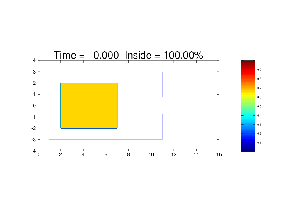
v⁡(ρ)=6​(1−ρ)η⁡(x)=[1−(x1r)2]3​[1−(x2r)2]3​χ[−r,r]2​(x),r=0.6ρ0​(x)=0.75​χ[2,7]×[−2,2]​(x)ε=0.4\begin{array}[]{@{}rcl@{}}v(\rho)&=&6(1-\rho)\\ \eta(x)&=&\left[1-\left(\frac{x_{1}}{r}\right)^{2}\right]^{3}\left[1-\left(\frac{x_{2}}{r}\right)^{2}\right]^{3}\,{\chi_{[-r,r]^{2}}}(x)\,,\\ r&=&0.6\\ \rho_{0}(x)&=&0.75\,{\chi_{[2,7]\times[-2,2]}}(x)\\ \varepsilon&=&0.4\\ \\ \end{array} (4.2)
Refer to caption
Figure 4: Initial datum and room geometry considered in § 4.2.

Keeping the above parameters fixed, as well as the outer walls of the room, we insert various obstacles (columns) to direct the movement of the crowd.

First, Figure 5, first line, shows an integration of the case with two columns that direct people towards the exit.

Refer to caption
Refer to caption
Refer to caption
Refer to caption
Refer to caption
Refer to caption
Figure 5: Solution to (1.1)–(1.2)–(3.4)–(4.2) with different geometries, computed at time t=2.521t=2.521, 5.0435.043 and 7.5637.563.

The number of lanes self adapts to the available space, with three lanes merging into one before the bottleneck. On the second line of Figure 5, the insertion of three columns in these positions delays but does not avoid the congestion at the exit. Those individuals that pass through the bottleneck are favored in exiting the room.

In Figure 6, first line, the insertion of four columns is more successful. Note, in the first two diagrams, that the number of lanes changes from 77 before the bottleneck, to 44 in between it. The individuals that do not pass through the bottleneck are penalized by the high density they meet near the door jambs.

Refer to caption
Refer to caption
Refer to caption
Refer to caption
Refer to caption
Refer to caption
Figure 6: Solution to (1.1)–(1.2)–(3.4)–(4.2) with different geometries, computed at time t=2.521t=2.521, 5.0435.043 and 7.5637.563.

Finally, on the second line in Figure 6, an asymmetric layout hinders the lanes’ pattern.

4.3 On the Rise of Singularities

A typical feature of conservation laws is the possible rise of singularities, see for instance [3, Example 1.4]. The nonlocal equation (1.1) shares this characteristic. Indeed, assume ρ=ρ⁡(t,x)\rho=\rho(t,x) is a given solution to (1.1), smooth up to time T>0T>0. Then, setting w⁡(t,x)=(ν⁡(x)+(ℐ⁡(t))​(x))w(t,x)=\left(\nu(x)+\left(\mathcal{I}(t)\right)(x)\right), simple computations lead to the following equation for the space derivative ρj\rho_{j} of ρ\rho in the direction xjx_{j}, for j=1,…,Nj=1,\ldots,N:

∂tρj+(div​ρj)​q′​w=(ρj)2​q′′​w+ρj​q′′​∑i≠j(∂iρ)​w+ρj​q′​div​w+q′​∑(∂iρ)​∂jw+q​∂jdiv​w.\partial_{t}\rho_{j}+(\mathinner{\rm div}\rho_{j})\,q^{\prime}\,w=(\rho_{j})^{2}\,q^{\prime\prime}\,w+\rho_{j}\,q^{\prime\prime}\,\sum_{i\neq j}(\partial_{i}\rho)\,w+\rho_{j}\,q^{\prime}\,\mathinner{\rm div}w+q^{\prime}\,\sum(\partial_{i}\rho)\,\partial_{j}w+q\,\partial_{j}\mathinner{\rm div}w\,.

The first term in the right hand side is quadratic in ρj\rho_{j}, showing that a blow up of ρj\rho_{j} may take place in finite time.

Refer to caption
Refer to caption
Figure 7: Left, the initial datum and, right, the solution to (1.1)–(1.2)–(4.3) at time t=1t=1. Note the formation of vertical faces in the initially smooth distribution.

Moreover, we consider (1.1) with ℐ\mathcal{I} as in (1.2) and

v⁡(ρ)=1−ρ,η⁡(x,y)=(1−16x2)3(1−16y2)3χ[−1/4,1/4]2(x,y),ν⁡(x)=0,ρ0​(x,y)=(1−4x2/9)2(1−4y2/9)2χ[−3/2,3/2]2(x,y),ε=−1\begin{array}[]{rcl@{\quad}rcl}v(\rho)&=&1-\rho\,,&\eta(x,y)&=&(1-16x^{2})^{3}\,(1-16y^{2})^{3}\,{\chi_{[-1/4,1/4]^{2}}}(x,y)\,,\\ \nu(x)&=&0\,,&\rho_{0}(x,y)&=&(1-4x^{2}/9)^{2}\,(1-4y^{2}/9)^{2}\,{\chi_{[-3/2,3/2]^{2}}}(x,y)\,,\end{array}\hskip 10.00002pt\varepsilon=-1 (4.3)

and we obtain the solution in Figure 7.

5 Technical Details

5.1 Existence and uniqueness

Proof of Lemma 2.2.  Let q⁡(ρ)=ρ​v​(ρ)q(\rho)=\rho\,v(\rho). Thanks to (ν\boldsymbol{\nu}), the assumptions on rr and (I.1), we have for all M>0M>0

∂ρf⁡(t,x,ρ)=q′​(ρ)​(ν⁡(x)+ℐ⁡(r⁡(t))​(x));∂ρf∈𝐋∞​([0,T]×ℝN×[−M,M],ℝN);div​f​(t,x,ρ)=q⁡(ρ)​div​(ν⁡(x)+ℐ⁡(r⁡(t))​(x));div​f∈𝐋∞​([0,T]×ℝN×[−M,M],ℝ).\begin{array}[]{r@{\;}c@{\;}lr@{\;}c@{\;}l}\partial_{\rho}f(t,x,\rho)&=&q^{\prime}(\rho)\,\left(\nu(x)+\mathcal{I}\left(r(t)\right)(x)\right);&\partial_{\rho}f&\in&{\mathbf{L}^{\infty}}([0,T]\times{\mathbb{R}}^{N}\times[-M,M];{\mathbb{R}}^{N})\,;\\ \mathinner{\rm div}f(t,x,\rho)&=&q(\rho)\,\mathinner{\rm div}\left(\nu(x)+\mathcal{I}\left(r(t)\right)(x)\right);&\mathinner{\rm div}f&\in&{\mathbf{L}^{\infty}}([0,T]\times{\mathbb{R}}^{N}\times[-M,M];{\mathbb{R}})\,.\end{array}

Thus, we can apply Kružkov Theorem [24, Theorem 5 & §5.4] and ensure that (2.2) admits a unique Kružkov solution ρ∈𝐋∞​(ℝ+,𝐋1​(ℝN,ℝ))\rho\in{\mathbf{L}^{\infty}}\left({\mathbb{R}^{+}};{\mathbf{L}^{1}}({\mathbb{R}}^{N};{\mathbb{R}})\right), which is continuous from the right in time.   □\square

Lemma 5.1.

Let ρ0∈𝐋1​(ℝN,[0,R])\rho_{0}\in{\mathbf{L}^{1}}({\mathbb{R}}^{N};[0,R]), r∈𝐂0​(ℝ+,𝐋1​(ℝN,[0,R]))r\in\mathbf{C}^{0}\left({\mathbb{R}^{+}};{\mathbf{L}^{1}}({\mathbb{R}}^{N};[0,R])\right). Under hypotheses (v)–(𝛎\boldsymbol{\nu})–(I.1), the Cauchy problem (2.2) admits a unique weak entropy solution ρ\rho, with ρ∈𝐂0​(ℝ+,𝐋1​(ℝN,[0,R]))\rho\in\mathbf{C}^{0}\left({\mathbb{R}^{+}};{\mathbf{L}^{1}}({\mathbb{R}}^{N};[0,R])\right) satisfying, for all t∈ℝ+t\in{\mathbb{R}^{+}},

‖ρ⁡(t)‖𝐋1=‖ρ0‖𝐋1.{\left\|\rho(t)\right\|}_{{\mathbf{L}^{1}}}={\left\|\rho_{0}\right\|}_{{\mathbf{L}^{1}}}\,. (5.1)

Assume, in addition, that (I.2) is satisfied. Then, ρ0∈𝐁𝐕⁡(ℝN,[0,R])\rho_{0}\in\mathbf{BV}({\mathbb{R}}^{N};[0,R]) implies ρ⁡(t)∈𝐁𝐕⁡(ℝN,[0,R])\rho(t)\in\mathbf{BV}({\mathbb{R}}^{N};[0,R]) for all time t⩾0t\geqslant 0. Moreover, the following bound is satisfied

TV(ρ(t))⩽[TV(ρ0)+tNWN‖q‖𝐋∞​([0,R])(‖∇divν‖𝐋1+CI(‖r‖𝐋∞​([0,T],𝐋1)))]eκ0∗​t,\mathinner{\rm TV}\left(\rho(t)\right)\leqslant\left[\mathinner{\rm TV}(\rho_{0})+t\,NW_{N}{\left\|q\right\|}_{{\mathbf{L}^{\infty}}([0,R])}\left({\left\|\nabla\mathinner{\rm div}\nu\right\|}_{{\mathbf{L}^{1}}}+C_{I}({\left\|r\right\|}_{{\mathbf{L}^{\infty}}([0,T];{\mathbf{L}^{1}})})\right)\right]e^{\kappa_{0}^{*}t}, (5.2)

where WN=∫0π/2(cos⁡ϑ)N​d​ϑW_{N}=\int_{0}^{\pi/2}(\cos\vartheta)^{N}\mathinner{\mathrm{d}{\vartheta}} and the constant κ0∗\kappa_{0}^{*} is bounded above as follows:

κ0∗⩽(2​N+1)​‖q′‖𝐋∞​([0,R])​(‖∇ν‖𝐋∞+CI​(‖r‖𝐋∞​([0,T],𝐋1))).\kappa_{0}^{*}\leqslant(2N+1){\left\|q^{\prime}\right\|}_{{\mathbf{L}^{\infty}}([0,R])}\left({\left\|\nabla\nu\right\|}_{{\mathbf{L}^{\infty}}}+C_{I}({\left\|r\right\|}_{{\mathbf{L}^{\infty}}([0,T];{\mathbf{L}^{1}})})\right)\,.

Proof.  Below we denote q⁡(ρ)=ρ​v​(ρ)q(\rho)=\rho\,v(\rho), so that f⁡(t,x,ρ)=q⁡(ρ)​(ν⁡(x)+(ℐ⁡(r⁡(t)))​(x))f(t,x,\rho)=q(\rho)\,\left(\nu(x)+\left(\mathcal{I}\left(r(t)\right)\right)(x)\right). The existence of a solution follows from Lemma 2.2. The rest of the proof is obtained through the following steps.

Estimates in 𝐋1{\mathbf{L}^{1}} and 𝐋∞{\mathbf{L}^{\infty}}.

Since ρ\rho is a solution to a conservation law, (5.1) is immediately satisfied.

Besides, ρ≡0\rho\equiv 0 and ρ≡R\rho\equiv R are solutions to (2.2) associated respectively to the constant initial conditions ρ0≡0\rho_{0}\equiv 0 and ρ0≡R\rho_{0}\equiv R. Hence, we can apply the comparison Theorem [24, Theorem 3] and obtain that if the initial condition takes value in [0,R][0,R], then the solution takes values in [0,R][0,R], so that ρ∈𝐋∞​(ℝ+,𝐋1​(ℝN,[0,R]))\rho\in{\mathbf{L}^{\infty}}\left({\mathbb{R}^{+}};{\mathbf{L}^{1}}({\mathbb{R}}^{N};[0,R])\right).

Continuity in time.

Thanks to [9, Remark 2.4] or [25, Corollary 2.4], ρ\rho is continuous in time if, for any T>0T>0,

‖q‖𝐋∞​([0,R])​∫0T∫ℝN|div⁡(ν⁡(x)+(ℐ⁡(r⁡(t)))​(x))|​d​x​d​t<∞.{\left\|q\right\|}_{{\mathbf{L}^{\infty}}([0,R])}\int_{0}^{T}\int_{{\mathbb{R}}^{N}}{\left|\mathinner{\rm div}\left(\nu(x)+\left(\mathcal{I}\left(r(t)\right)\right)(x)\right)\right|}\mathinner{\mathrm{d}{x}}\mathinner{\mathrm{d}{t}}<\infty\,. (5.3)

We have, thanks to (I.1), for all t⩾0t\geqslant 0

‖div⁡(ν+ℐ⁡(r⁡(t)))‖𝐋1⩽‖div​ν‖𝐋1+CI​(‖r⁡(t)‖𝐋1).{\left\|\mathinner{\rm div}\left(\nu+\mathcal{I}\left(r(t)\right)\right)\right\|}_{{\mathbf{L}^{1}}}\leqslant{\left\|\mathinner{\rm div}\nu\right\|}_{{\mathbf{L}^{1}}}+C_{I}({\left\|r(t)\right\|}_{{\mathbf{L}^{1}}})\,.

Hence, condition (5.3) is satisfied under hypotheses (v)–(ν\boldsymbol{\nu})–(I.1) and we also obtain ρ∈𝐂0​(ℝ+,𝐋1​(ℝN,[0,R]))\rho\in\mathbf{C}^{0}({\mathbb{R}^{+}};{\mathbf{L}^{1}}({\mathbb{R}}^{N};[0,R])).

Estimate in 𝐁𝐕\mathbf{BV}.

To prove the bound on the TV\mathinner{\rm TV} norm we use [25, Theorem 2.2]. To this aim, we have to check that for any T>0T>0,

∇∂ρf∈𝐋∞([0,T]×ℝN×[0,R];ℝN×N) and ∫0T∫ℝN‖∇divf(t,x,⋅)‖𝐋∞​([0,R])d​xd​t<∞.\nabla\partial_{\rho}f\in{\mathbf{L}^{\infty}}([0,T]\times{\mathbb{R}}^{N}\times[0,R];{\mathbb{R}}^{N\times N})\hskip 10.00002pt\mbox{ and }\hskip 10.00002pt\int_{0}^{T}\!\!\!\int_{{\mathbb{R}}^{N}}{\left\|\nabla\mathinner{\rm div}f(t,x,\cdot)\right\|}_{{\mathbf{L}^{\infty}}([0,R])}\mathinner{\mathrm{d}{x}}\mathinner{\mathrm{d}{t}}<\infty\,.

Note first that ∇∂ρf(t,x,ρ)=q′(ρ)∇(ν+ℐ(r(t)))\nabla\partial_{\rho}f(t,x,\rho)=q^{\prime}(\rho)\,\nabla\left(\nu+\mathcal{I}\left(r(t)\right)\right). Hence, thanks to (v)–(ν\boldsymbol{\nu}) and (I.1), we have

‖∇∂ρf(t,x,ρ)‖𝐋∞⩽‖q′‖𝐋∞​([0,R])(‖∇ν‖𝐋∞+CI(‖r(t)‖𝐋1)),{\left\|\nabla\partial_{\rho}f(t,x,\rho)\right\|}_{{\mathbf{L}^{\infty}}}\leqslant{\left\|q^{\prime}\right\|}_{{\mathbf{L}^{\infty}}([0,R])}\left({\left\|\nabla\nu\right\|}_{{\mathbf{L}^{\infty}}}+C_{I}({\left\|r(t)\right\|}_{{\mathbf{L}^{1}}})\right)\,,

Thanks to (v)–(ν\boldsymbol{\nu}) and (I.2), we have, for all t⩾0t\geqslant 0

‖∇div(ν+ℐ(r(t)))‖𝐋1⩽‖∇divν‖𝐋1+CI(‖r(t)‖𝐋1).{\left\|\nabla\mathinner{\rm div}\left(\nu+\mathcal{I}\left(r(t)\right)\right)\right\|}_{{\mathbf{L}^{1}}}\leqslant{\left\|\nabla\mathinner{\rm div}\nu\right\|}_{{\mathbf{L}^{1}}}+C_{I}({\left\|r(t)\right\|}_{{\mathbf{L}^{1}}})\,.

Applying [25, Theorem 2.2], we obtain

κ0∗\displaystyle\kappa_{0}^{*} =\displaystyle= (2N+1)‖∇∂ρf‖𝐋∞\displaystyle(2N+1){\left\|\nabla\partial_{\rho}f\right\|}_{{\mathbf{L}^{\infty}}}
⩽\displaystyle\leqslant (2​N+1)​‖q′‖𝐋∞​([0,R])​(‖∇ν‖𝐋∞+CI​(‖r‖𝐋∞​([0,T],𝐋1))),\displaystyle(2N+1)\,{\left\|q^{\prime}\right\|}_{{\mathbf{L}^{\infty}}([0,R])}\left({\left\|\nabla\nu\right\|}_{{\mathbf{L}^{\infty}}}+C_{I}({\left\|r\right\|}_{{\mathbf{L}^{\infty}}([0,T];{\mathbf{L}^{1}})})\right)\,,
TV⁡(ρ⁡(t))\displaystyle\mathinner{\rm TV}(\rho(t)) ⩽\displaystyle\leqslant TV⁡(ρ0)​eκ0∗​t\displaystyle\mathinner{\rm TV}(\rho_{0})\,e^{\kappa_{0}^{*}t}
+teκ0∗​tNWN‖q‖𝐋∞​([0,R])(‖∇divν‖𝐋1+CI(‖r‖𝐋∞​([0,T],𝐋1))),\displaystyle+te^{\kappa_{0}^{*}t}NW_{N}{\left\|q\right\|}_{{\mathbf{L}^{\infty}}([0,R])}\left({\left\|\nabla\mathinner{\rm div}\nu\right\|}_{{\mathbf{L}^{1}}}+C_{I}({\left\|r\right\|}_{{\mathbf{L}^{\infty}}([0,T];{\mathbf{L}^{1}})})\right)\,,

completing the proof.   □\square

Proof of Theorem 2.3.  Thanks to Lemma 5.1, under hypotheses (v)–(ν\boldsymbol{\nu}) and (I), for any r∈𝐂0​([0,T],𝐋1​(ℝN,[0,R]))r\in\mathbf{C}^{0}\left([0,T];{\mathbf{L}^{1}}({\mathbb{R}}^{N};[0,R])\right) there exists a unique solution ρ∈𝐂0​(ℝ+,𝐋1​(ℝN,[0,R]))\rho\in\mathbf{C}^{0}\left({\mathbb{R}^{+}};{\mathbf{L}^{1}}({\mathbb{R}}^{N};[0,R])\right) to (2.2) satisfying (5.1)–(5.2). For any time T>0T>0, introduce the space

X(T)={r∈𝐂0([0,T];𝐋1(ℝN;[0,R])):∀t∈[0,T],‖r(t)‖𝐋1⩽‖ρ0‖𝐋1}.X(T)=\left\{r\in\mathbf{C}^{0}\left([0,T];{\mathbf{L}^{1}}({\mathbb{R}}^{N};[0,R])\right)\colon\forall\,t\in[0,T],{\left\|r(t)\right\|}_{{\mathbf{L}^{1}}}\leqslant{\left\|\rho_{0}\right\|}_{{\mathbf{L}^{1}}}\right\}\,.

Note that X⁡(T)X(T) is a Banach space with respect to the norm ‖r‖X⁡(T)=supt∈[0,T]‖r⁡(t)‖𝐋1{\left\|r\right\|}_{X(T)}=\sup_{t\in[0,T]}{\left\|r(t)\right\|}_{{\mathbf{L}^{1}}}. Let 𝒬\mathcal{Q} be the map that associates to r∈X⁡(T)r\in X(T) the solution ρ∈X⁡(T)\rho\in X(T) to (2.2). We want to find a condition on TT so that 𝒬\mathcal{Q} is a contraction.

Let r1,r2∈X⁡(T)r_{1},r_{2}\in X(T). To apply [25, Theorem 2.6], we have to check that, for all t∈[0,T]t\in[0,T],

∂ρ(f1−f2)∈𝐋∞​([0,T]×ℝN×[0,R],ℝN), and\displaystyle\partial_{\rho}(f_{1}-f_{2})\in{\mathbf{L}^{\infty}}([0,T]\times{\mathbb{R}}^{N}\times[0,R];{\mathbb{R}}^{N})\,,\mbox{ and}
∫0T∫ℝN‖div(f1−f2)(t,x,⋅)‖𝐋∞​([0,R])d​xd​t<+∞.\displaystyle\int_{0}^{T}\!\!\int_{{\mathbb{R}}^{N}}{\left\|\mathinner{\rm div}(f_{1}-f_{2})(t,x,\cdot)\right\|}_{{\mathbf{L}^{\infty}}([0,R])}\mathinner{\mathrm{d}{x}}\mathinner{\mathrm{d}{t}}<+\infty\,.

Thanks to (I.3) we have

‖∂ρ(f1−f2)‖𝐋∞=‖(ℐ⁡(r1)−ℐ⁡(r2))​q′‖𝐋∞⩽KI​‖q′‖𝐋∞​([0,R])​‖r1−r2‖𝐋∞​([0,T],𝐋1),\displaystyle{\left\|\partial_{\rho}(f_{1}-f_{2})\right\|}_{{\mathbf{L}^{\infty}}}={\left\|\left(\mathcal{I}(r_{1})-\mathcal{I}(r_{2})\right)q^{\prime}\right\|}_{{\mathbf{L}^{\infty}}}\leqslant K_{I}\,{\left\|q^{\prime}\right\|}_{{\mathbf{L}^{\infty}}([0,R])}\,{\left\|r_{1}-r_{2}\right\|}_{{\mathbf{L}^{\infty}}([0,T];{\mathbf{L}^{1}})}\,,
∫0T∫ℝN‖div(f1−f2)(t,x,⋅)‖𝐋∞​([0,R])d​xd​t⩽TKI‖q‖𝐋∞​([0,R])‖r1−r2‖𝐋∞​([0,T],𝐋1).\displaystyle\int_{0}^{T}\!\!\int_{{\mathbb{R}}^{N}}{\left\|\mathinner{\rm div}(f_{1}-f_{2})(t,x,\cdot)\right\|}_{{\mathbf{L}^{\infty}}([0,R])}\mathinner{\mathrm{d}{x}}\mathinner{\mathrm{d}{t}}\leqslant TK_{I}\,{\left\|q\right\|}_{{\mathbf{L}^{\infty}}([0,R])}\,{\left\|r_{1}-r_{2}\right\|}_{{\mathbf{L}^{\infty}}([0,T];{\mathbf{L}^{1}})}\,.

Hence, we get for all t⩾0t\geqslant 0

‖(ρ1−ρ2)​(t)‖𝐋1\displaystyle{\left\|(\rho_{1}-\rho_{2})(t)\right\|}_{{\mathbf{L}^{1}}}
⩽\displaystyle\leqslant t​KI​‖q‖𝐖1,∞​([0,R])​‖r1−r2‖𝐋∞​([0,T],𝐋1)\displaystyle t\,K_{I}{\left\|q\right\|}_{{\mathbf{W}^{1,\infty}}([0,R])}{\left\|r_{1}-r_{2}\right\|}_{{\mathbf{L}^{\infty}}([0,T];{\mathbf{L}^{1}})}
×[1+eκ0∗​t(TV(ρ0)+N​WN2t‖q‖𝐋∞​([0,R])(‖∇divν‖𝐋1+CI(‖r‖𝐋∞​([0,T],𝐋1))))].\displaystyle\times\big[1+e^{\kappa_{0}^{*}t}\left(\mathinner{\rm TV}(\rho_{0})+\frac{NW_{N}}{2}\,t\,{\left\|q\right\|}_{{\mathbf{L}^{\infty}}([0,R])}\left({\left\|\nabla\mathinner{\rm div}\nu\right\|}_{{\mathbf{L}^{1}}}+C_{I}({\left\|r\right\|}_{{\mathbf{L}^{\infty}}([0,T];{\mathbf{L}^{1}})})\right)\right)\big]\,.

Denoting

k\displaystyle k =\displaystyle= (2​N+1)​‖q′‖𝐋∞​([0,R])​(‖∇ν‖𝐋∞+CI​(‖ρ0‖𝐋1)),\displaystyle(2N+1){\left\|q^{\prime}\right\|}_{{\mathbf{L}^{\infty}}([0,R])}\left({\left\|\nabla\nu\right\|}_{{\mathbf{L}^{\infty}}}+C_{I}({\left\|\rho_{0}\right\|}_{{\mathbf{L}^{1}}})\right)\,, (5.4)
C1\displaystyle C_{1} =\displaystyle= KI​‖q‖𝐖1,∞​([0,R]),\displaystyle K_{I}\,{\left\|q\right\|}_{{\mathbf{W}^{1,\infty}}([0,R])}\,,
C2\displaystyle C_{2} =\displaystyle= N​WN2‖q‖𝐋∞​([0,R])(‖∇divν‖𝐋1+CI(‖ρ0‖𝐋1)).\displaystyle\frac{NW_{N}}{2}{\left\|q\right\|}_{{\mathbf{L}^{\infty}}([0,R])}\left({\left\|\nabla\mathinner{\rm div}\nu\right\|}_{{\mathbf{L}^{1}}}+C_{I}({\left\|\rho_{0}\right\|}_{{\mathbf{L}^{1}}})\right)\,.

The above estimate can be written

‖(ρ1−ρ2)​(t)‖𝐋1⩽C1​t​‖r1−r2‖𝐋∞​([0,T],𝐋1)​(1+ek​t​(TV⁡(ρ0)+C2​t)),{\left\|(\rho_{1}-\rho_{2})(t)\right\|}_{{\mathbf{L}^{1}}}\leqslant C_{1}\,t\,{\left\|r_{1}-r_{2}\right\|}_{{\mathbf{L}^{\infty}}([0,T];{\mathbf{L}^{1}})}\left(1+e^{kt}\left(\mathinner{\rm TV}(\rho_{0})+C_{2}t\right)\right)\,,

We choose now TT so that

C1​T​(1+ek​T​(TV⁡(ρ0)+C2​T))=12C_{1}\,T\,\left(1+e^{kT}\left(\mathinner{\rm TV}(\rho_{0})+C_{2}\,T\right)\right)=\frac{1}{2}

and, applying Banach Fixed Point Theorem, we obtain a unique fixed point for 𝒬\mathcal{Q} on X⁡(T)X(T).

We now iterate the procedure above. To this aim, we use the total variation estimate (5.2)

TV⁡(ρ⁡(t))⩽(TV⁡(ρ0)+2​C2​t)​ek​t,\mathinner{\rm TV}\left(\rho(t)\right)\leqslant\left(\mathinner{\rm TV}(\rho_{0})+2\,C_{2}t\right)e^{kt},

and, given TnT_{n}, we recursively define Tn+1T_{n+1} so that

C1​(Tn+1−Tn)​(1+ek​Tn+1​TV​(ρ0)+C2​ek⁡(Tn+1−Tn)​(2​Tn​ek​Tn+Tn+1−Tn))=12C_{1}\,(T_{n+1}-T_{n})\left(1+e^{kT_{n+1}}\mathinner{\rm TV}(\rho_{0})+C_{2}\,e^{k(T_{n+1}-T_{n})}(2T_{n}e^{kT_{n}}+T_{n+1}-T_{n})\right)=\frac{1}{2}

and the above procedure ensures the existence of a fixed point on the interval [Tn,Tn+1][T_{n},T_{n+1}].

The sequence TnT_{n} is strictly increasing. If it is bounded, then the latter relation above yields 0=1/20=1/2. Hence, Tn→∞T_{n}\to\infty when n→∞n\to\infty, completing the proof.   □\square

5.2 Stability

Proof of Theorem 2.4.  Here, we apply [25, Corollary 2.8] to compare the solutions ρ1\rho_{1} and ρ2\rho_{2} of (2.4). Let kk be as in (5.4). As in the proof of Theorem 2.3, (v)–(ν\boldsymbol{\nu})–(I) ensure that the set of hypotheses [25, (H1*)–(H2*)–(H3*)] are satisfied. Thus, for any t⩾0t\geqslant 0, we obtain

‖ρ1​(t)−ρ2​(t)‖𝐋1\displaystyle{\left\|\rho_{1}(t)-\rho_{2}(t)\right\|}_{{\mathbf{L}^{1}}}
⩽\displaystyle\leqslant ‖ρ0,1−ρ0,2‖𝐋1\displaystyle{\left\|\rho_{0,1}-\rho_{0,2}\right\|}_{{\mathbf{L}^{1}}}
+[ek​t​TV​(ρ0,1)+N​WN​‖q1‖𝐋∞​([0,R])​∫0tek⁡(t−τ)​∫ℝN‖∇div​(ν1​(x)+ℐ1​(ρ1))‖​d​x​d​τ]\displaystyle+\big[e^{kt}\mathinner{\rm TV}(\rho_{0,1})+NW_{N}{\left\|q_{1}\right\|}_{{\mathbf{L}^{\infty}}([0,R])}\int_{0}^{t}e^{k(t-\tau)}\int_{{\mathbb{R}}^{N}}{\left\|\nabla\mathinner{\rm div}(\nu_{1}(x)+\mathcal{I}_{1}(\rho_{1}))\right\|}\mathinner{\mathrm{d}{x}}\mathinner{\mathrm{d}{\tau}}\big]
×∫0t‖q1′​(ρ)​(ν1​(x)+ℐ1​(ρ1))−q2′​(ρ)​(ν2​(x)+ℐ2​(ρ2))‖𝐋∞​(ℝN)​d​τ\displaystyle\hskip 20.00003pt\times\int_{0}^{t}{\left\|q_{1}^{\prime}(\rho)\left(\nu_{1}(x)+\mathcal{I}_{1}(\rho_{1})\right)-q_{2}^{\prime}(\rho)\left(\nu_{2}(x)+\mathcal{I}_{2}(\rho_{2})\right)\right\|}_{{\mathbf{L}^{\infty}}({\mathbb{R}}^{N})}\mathinner{\mathrm{d}{\tau}}
+∫0t∫ℝN‖q1(ρ)div(ν1(x)+ℐ1(ρ1))−q2(ρ)div(ν2(x)+ℐ2(ρ2))‖𝐋∞​([0,R])d​xd​τ\displaystyle+\int_{0}^{t}\int_{{\mathbb{R}}^{N}}{\left\|q_{1}(\rho)\mathinner{\rm div}\left(\nu_{1}(x)+\mathcal{I}_{1}(\rho_{1})\right)-q_{2}(\rho)\mathinner{\rm div}\left(\nu_{2}(x)+\mathcal{I}_{2}(\rho_{2})\right)\right\|}_{{\mathbf{L}^{\infty}}([0,R])}\mathinner{\mathrm{d}{x}}\mathinner{\mathrm{d}{\tau}}
⩽\displaystyle\leqslant ‖ρ0,1−ρ0,2‖𝐋1+[TV(ρ0,1)+tNWN‖q1‖𝐋∞​([0,R])(‖∇divν1‖𝐋1+CI(‖ρ0,1‖𝐋1))]\displaystyle{\left\|\rho_{0,1}-\rho_{0,2}\right\|}_{{\mathbf{L}^{1}}}+\big[\mathinner{\rm TV}(\rho_{0,1})+t\,NW_{N}{\left\|q_{1}\right\|}_{{\mathbf{L}^{\infty}}([0,R])}\left({\left\|\nabla\mathinner{\rm div}\nu_{1}\right\|}_{{\mathbf{L}^{1}}}+C_{I}({\left\|\rho_{0,1}\right\|}_{{\mathbf{L}^{1}}})\right)\big]
×(t​‖q1′−q2′‖𝐋∞​([0,R])​‖ν1+ℐ1​(ρ1)‖𝐋∞CLOSE\displaystyle\hskip 20.00003pt\times\big(t\,{\left\|q_{1}^{\prime}-q_{2}^{\prime}\right\|}_{{\mathbf{L}^{\infty}}([0,R])}{\left\|\nu_{1}+\mathcal{I}_{1}(\rho_{1})\right\|}_{{\mathbf{L}^{\infty}}}
+t​‖q2′‖𝐋∞​([0,R])​‖ν1−ν2+ℐ1​(ρ1)−ℐ2​(ρ1)‖𝐋∞\displaystyle\hskip 20.00003pt\hskip 20.00003pt+t\,{\left\|q_{2}^{\prime}\right\|}_{{\mathbf{L}^{\infty}}([0,R])}{\left\|\nu_{1}-\nu_{2}+\mathcal{I}_{1}(\rho_{1})-\mathcal{I}_{2}(\rho_{1})\right\|}_{{\mathbf{L}^{\infty}}}
+‖q2′‖𝐋∞​([0,R])∫0t‖ℐ2(ρ1(τ))−ℐ2(ρ2(τ))‖𝐋∞d​τ)\displaystyle\hskip 20.00003pt\hskip 20.00003pt+{\left\|q_{2}^{\prime}\right\|}_{{\mathbf{L}^{\infty}}([0,R])}\int_{0}^{t}{\left\|\mathcal{I}_{2}\left(\rho_{1}(\tau)\right)-\mathcal{I}_{2}\left(\rho_{2}(\tau)\right)\right\|}_{{\mathbf{L}^{\infty}}}\mathinner{\mathrm{d}{\tau}}\big)
+t​‖q2‖𝐋∞​([0,R])​‖div⁡(ν1−ν2+ℐ1​(ρ1)−ℐ2​(ρ1))‖𝐋1\displaystyle+t{\left\|q_{2}\right\|}_{{\mathbf{L}^{\infty}}([0,R])}{\left\|\mathinner{\rm div}\left(\nu_{1}-\nu_{2}+\mathcal{I}_{1}(\rho_{1})-\mathcal{I}_{2}(\rho_{1})\right)\right\|}_{{\mathbf{L}^{1}}}
+t​‖q1−q2‖𝐋∞​([0,R])​‖div⁡(ν1+ℐ1​(ρ1))‖𝐋1+‖q2‖𝐋∞​([0,R])​∫0t|div⁡(ℐ2​(ρ1)−ℐ2​(ρ2))|​d​τ.\displaystyle+t{\left\|q_{1}-q_{2}\right\|}_{{\mathbf{L}^{\infty}}([0,R])}{\left\|\mathinner{\rm div}(\nu_{1}+\mathcal{I}_{1}(\rho_{1}))\right\|}_{{\mathbf{L}^{1}}}+{\left\|q_{2}\right\|}_{{\mathbf{L}^{\infty}}([0,R])}\int_{0}^{t}{\left|\mathinner{\rm div}\left(\mathcal{I}_{2}(\rho_{1})-\mathcal{I}_{2}(\rho_{2})\right)\right|}\mathinner{\mathrm{d}{\tau}}.

Hence, denoting

a⁡(t)\displaystyle a(t) =\displaystyle= TV(ρ0,1)+tNWN‖q1‖𝐋∞​([0,R])(‖∇divν1‖𝐋1+CI(‖ρ0,1‖𝐋1))\displaystyle\mathinner{\rm TV}(\rho_{0,1})+t\,NW_{N}\,{\left\|q_{1}\right\|}_{{\mathbf{L}^{\infty}}([0,R])}\left({\left\|\nabla\mathinner{\rm div}\nu_{1}\right\|}_{{\mathbf{L}^{1}}}+C_{I}({\left\|\rho_{0,1}\right\|}_{{\mathbf{L}^{1}}})\right)
b⁡(t)\displaystyle b(t) =\displaystyle= KI​(‖q2′‖𝐋∞​([0,R])​ek​t​a​(t)+‖q2‖𝐋∞​([0,R]))\displaystyle K_{I}\left({\left\|q_{2}^{\prime}\right\|}_{{\mathbf{L}^{\infty}}([0,R])}e^{kt}a(t)+{\left\|q_{2}\right\|}_{{\mathbf{L}^{\infty}}([0,R])}\right)
γ1\displaystyle\gamma_{1} =\displaystyle= ‖q1′−q2′‖𝐋∞​([0,R])​(‖ν1‖𝐋∞+CI​(‖ρ0,1‖𝐋1))+‖q2′‖𝐋∞​([0,R])​‖ν1−ν2‖𝐋∞\displaystyle{\left\|q_{1}^{\prime}-q_{2}^{\prime}\right\|}_{{\mathbf{L}^{\infty}}([0,R])}\left({\left\|\nu_{1}\right\|}_{{\mathbf{L}^{\infty}}}+C_{I}({\left\|\rho_{0,1}\right\|}_{{\mathbf{L}^{1}}})\right)+{\left\|q_{2}^{\prime}\right\|}_{{\mathbf{L}^{\infty}}([0,R])}{\left\|\nu_{1}-\nu_{2}\right\|}_{{\mathbf{L}^{\infty}}}
+‖q2′‖𝐋∞​([0,R])supρ∈𝐋1​(ℝN,[0,R])‖ℐ1(ρ)−ℐ2(ρ)‖𝐋∞\displaystyle\hskip 20.00003pt+{\left\|q_{2}^{\prime}\right\|}_{{\mathbf{L}^{\infty}}([0,R])}\sup_{\rho\in{\mathbf{L}^{1}}({\mathbb{R}}^{N};[0,R])}{\left\|\mathcal{I}_{1}(\rho)-\mathcal{I}_{2}(\rho)\right\|}_{{\mathbf{L}^{\infty}}}
γ2\displaystyle\gamma_{2} =\displaystyle= ‖q1−q2‖𝐋∞​([0,R])​(‖div​ν1‖𝐋1+CI​(‖ρ0,1‖𝐋1))\displaystyle{\left\|q_{1}-q_{2}\right\|}_{{\mathbf{L}^{\infty}}([0,R])}\left({\left\|\mathinner{\rm div}\nu_{1}\right\|}_{{\mathbf{L}^{1}}}+C_{I}({\left\|\rho_{0,1}\right\|}_{{\mathbf{L}^{1}}})\right)
+‖q2‖𝐋∞​([0,R])​(‖div⁡(ν1−ν2)‖𝐋1+supρ∈𝐋1​(ℝN,[0,R])‖div​ℐ1​(ρ)−div​ℐ2​(ρ)‖𝐋1)\displaystyle+{\left\|q_{2}\right\|}_{{\mathbf{L}^{\infty}}([0,R])}\left({\left\|\mathinner{\rm div}(\nu_{1}-\nu_{2})\right\|}_{{\mathbf{L}^{1}}}+\sup_{\rho\in{\mathbf{L}^{1}}({\mathbb{R}}^{N};[0,R])}{\left\|\mathinner{\rm div}\mathcal{I}_{1}(\rho)-\mathinner{\rm div}\mathcal{I}_{2}(\rho)\right\|}_{{\mathbf{L}^{1}}}\right)

we get

‖ρ1−ρ2​(t)‖𝐋1⩽‖ρ0,1−ρ0,2‖𝐋1+γ1​t​ek​t​a​(t)+t​γ2+b⁡(t)​∫0t‖ρ1−ρ2​(τ)‖​d​τ.{\left\|\rho_{1}-\rho_{2}(t)\right\|}_{{\mathbf{L}^{1}}}\leqslant{\left\|\rho_{0,1}-\rho_{0,2}\right\|}_{{\mathbf{L}^{1}}}+\gamma_{1}\,t\,e^{kt}\,a(t)+t\,\gamma_{2}+b(t)\int_{0}^{t}{\left\|\rho_{1}-\rho_{2}(\tau)\right\|}\,\mathinner{\mathrm{d}{\tau}}\,.

By Gronwall Lemma, we obtain

‖ρ1−ρ2​(t)‖𝐋1\displaystyle{\left\|\rho_{1}-\rho_{2}(t)\right\|}_{{\mathbf{L}^{1}}} ⩽\displaystyle\leqslant ‖ρ0,1−ρ0,2‖𝐋1+γ1​t​ek​t​a​(t)+t​γ2\displaystyle{\left\|\rho_{0,1}-\rho_{0,2}\right\|}_{{\mathbf{L}^{1}}}+\gamma_{1}\,t\,e^{kt}\,a(t)+t\,\gamma_{2}
+b(t)e∫0tb⁡(u)​d​u∫0te−∫0τb(u)d​u(‖ρ0,1−ρ0,2‖𝐋1+γ1τek​τa(τ)+τγ2)d​τ.\displaystyle+b(t)e^{\int_{0}^{t}b(u)\mathinner{\mathrm{d}{u}}}\int_{0}^{t}e^{-\int_{0}^{\tau}b(u)\mathinner{\mathrm{d}{u}}}({\left\|\rho_{0,1}-\rho_{0,2}\right\|}_{{\mathbf{L}^{1}}}+\gamma_{1}\tau e^{k\tau}\,a(\tau)+\tau\gamma_{2})\mathinner{\mathrm{d}{\tau}}\,.

Noting that

e−∫0tb(u)d​u+b(t)∫0te−∫0τb(u)d​ud​τ⩽b⁡(t)b⁡(0)e^{-\int_{0}^{t}b(u)\mathinner{\mathrm{d}{u}}}+b(t)\int_{0}^{t}e^{-\int_{0}^{\tau}b(u)\mathinner{\mathrm{d}{u}}}\mathinner{\mathrm{d}{\tau}}\leqslant\frac{b(t)}{b(0)}

we get

‖ρ1−ρ2​(t)‖𝐋1\displaystyle{\left\|\rho_{1}-\rho_{2}(t)\right\|}_{{\mathbf{L}^{1}}} ⩽\displaystyle\leqslant (‖ρ0,1−ρ0,2‖𝐋1+γ1​t​ek​t​a​(t)+t​γ2)​b⁡(t)b⁡(0)​et​b​(t)\displaystyle\left({\left\|\rho_{0,1}-\rho_{0,2}\right\|}_{{\mathbf{L}^{1}}}+\gamma_{1}\,t\,e^{kt}\,a(t)+t\,\gamma_{2}\right)\frac{b(t)}{b(0)}e^{tb(t)}

completing the proof.   □\square

5.3 Driving examples

Proof of Proposition 3.1.  Let ρ\rho solve (1.1) in the sense of Definition 2.1. Define w⁡(t,x)=ν⁡(x)+(ℐ⁡(ρ⁡(t)))​(x)w(t,x)=\nu(x)+\left(\mathcal{I}\left(\rho(t)\right)\right)(x). Then, ρ∈𝐂0​([0,T],𝐋1​(ℝN,[0,R]))\rho\in\mathbf{C}^{0}([0,T];{\mathbf{L}^{1}}({\mathbb{R}}^{N};[0,R])) is also a weak solution to (2.1). Then, set as above q⁡(ρ)=ρ​v​(ρ)q(\rho)=\rho\,v(\rho) and, for any φ∈𝐂c∞​(ℝ×ℝN,ℝ)\varphi\in\mathbf{C}_{c}^{\infty}({\mathbb{R}}\times{\mathbb{R}}^{N};{\mathbb{R}}), we have

∫ℝ∫ℝN(ρ​∂tφ+q⁡(ρ)​w​(t,x)⋅∇φ​(t,x))​d​x​d​t=0.\int_{\mathbb{R}}\int_{{\mathbb{R}}^{N}}\left(\rho\,\partial_{t}\varphi+q(\rho)\,w(t,x)\cdot\nabla\varphi(t,x)\right)\mathinner{\mathrm{d}{x}}\,\mathinner{\mathrm{d}{t}}=0\,.

Fix positive TT and MM. For α>0\alpha>0 define Yα∈𝐂∞​(ℝ,ℝ)Y_{\alpha}\in\mathbf{C}^{\infty}({\mathbb{R}};{\mathbb{R}}) so that Yα​(s)=0Y_{\alpha}(s)=0 for s⩽0s\leqslant 0, Yα​(s)=1Y_{\alpha}(s)=1 for s⩾αs\geqslant\alpha and Yα′​(s)⩾0Y_{\alpha}^{\prime}(s)\geqslant 0 for all ss. Let ζ⁡(t)=Yα​(t−α)−Yα​(t−T)\zeta(t)=Y_{\alpha}(t-\alpha)-Y_{\alpha}(t-T).

Call KM=B⁡(0,M)∖ΩK_{M}=B(0,M)\setminus\Omega. Set μ∈𝐂c∞​([−1,1],[0,1])\mu\in\mathbf{C}_{c}^{\infty}([-1,1];[0,1]) such that ∫ℝμ⁡(r)​d​r=1\int_{\mathbb{R}}\mu(r)\,\mathinner{\mathrm{d}{r}}=1. For ϑ>0\vartheta>0, let μϑ​(x)=1ϑN​μ​(‖x‖/ϑ)\mu_{\vartheta}(x)=\frac{1}{\vartheta^{N}}\,\mu\left({\left\|x\right\|}/\vartheta\right) and define ψ=χKM∗μϑ\psi={\chi_{K_{M}}}*\mu_{\vartheta}, the convolution being over all of ℝN{\mathbb{R}}^{N}. Note that ∇ψ=0\nabla\psi=0 on ℝN∖B⁡(∂KM,ϑ){\mathbb{R}}^{N}\setminus B(\partial K_{M},\vartheta). If x∈B⁡(∂KM,ϑ)x\in B(\partial K_{M},\vartheta), we have

∇ψ(x)=∫KM∇μϑ(x−y)d​y=−∫∂KMμϑ(x−y)n~(y)d​σ​(y),\nabla\psi(x)=\int_{K_{M}}\nabla\mu_{\vartheta}(x-y)\,\mathinner{\mathrm{d}{y}}=-\int_{\partial K_{M}}\mu_{\vartheta}(x-y)\,\tilde{n}(y)\,\mathinner{\mathrm{d}{\sigma(y)}}\,,

where n~​(x)\tilde{n}(x) is the outer normal to KMK_{M} at any x∈∂KMx\in\partial K_{M}. Then, we choose φ⁡(t,x)=ζ⁡(t)​ψ​(x)\varphi(t,x)=\zeta(t)\,\psi(x). Clearly, φ∈𝐂c∞​(ℝ×ℝN,ℝ)\varphi\in\mathbf{C}_{c}^{\infty}({\mathbb{R}}\times{\mathbb{R}}^{N};{\mathbb{R}}). The definition of weak solution gives

0=∫ℝ∫ℝN(ρ(t,x)ζ′(t)ψ(x)+q(ρ(t,x))w(t,x)ζ(t)∇ψ(x))d​xd​t.0=\int_{{\mathbb{R}}}\int_{{\mathbb{R}}^{N}}\left(\rho(t,x)\,\zeta^{\prime}(t)\,\psi(x)+q\left(\rho(t,x)\right)\,w(t,x)\,\zeta(t)\,\nabla\psi(x)\right)\mathinner{\mathrm{d}{x}}\mathinner{\mathrm{d}{t}}\,.

Letting α→0\alpha\to 0, we obtain

0\displaystyle 0 =\displaystyle= ∫ℝN(ρ(0,x)−ρ(T,x))ψ(x)d​x+∫0T∫ℝNq(ρ(t,x))w(t,x)∇ψ(x)d​xd​t\displaystyle\int_{{\mathbb{R}}^{N}}\left(\rho(0,x)-\rho(T,x)\right)\psi(x)\,\mathinner{\mathrm{d}{x}}+\int_{0}^{T}\int_{{\mathbb{R}}^{N}}q\left(\rho(t,x)\right)\,w(t,x)\,\nabla\psi(x)\,\mathinner{\mathrm{d}{x}}\,\mathinner{\mathrm{d}{t}}
=\displaystyle= ∫ℝN(ρ⁡(0,x)−ρ⁡(T,x))​ψ​(x)​d​x\displaystyle\int_{{\mathbb{R}}^{N}}\left(\rho(0,x)-\rho(T,x)\right)\psi(x)\,\mathinner{\mathrm{d}{x}}
−∫0T∫ℝN∫∂KMq(ρ(t,x))w(t,x)⋅n~(y)μϑ(x−y)d​σ​(y)d​xd​t\displaystyle\hskip 20.00003pt-\int_{0}^{T}\int_{{\mathbb{R}}^{N}}\int_{\partial K_{M}}q\left(\rho(t,x)\right)w(t,x)\cdot\tilde{n}(y)\,\mu_{\vartheta}(x-y)\,\mathinner{\mathrm{d}{\sigma(y)}}\,\mathinner{\mathrm{d}{x}}\,\mathinner{\mathrm{d}{t}}
=\displaystyle= ∫ℝN(ρ⁡(0,x)−ρ⁡(T,x))​ψ​(x)​d​x\displaystyle\int_{{\mathbb{R}}^{N}}\left(\rho(0,x)-\rho(T,x)\right)\psi(x)\,\mathinner{\mathrm{d}{x}}
−∫0T∫∂KM∫B⁡(0,1)q(ρ(t,y+ϑz))w(t,y+ϑz)⋅n~(y)μ(‖z‖)d​zd​σ​(y)d​t.\displaystyle\hskip 20.00003pt-\int_{0}^{T}\int_{\partial K_{M}}\int_{B(0,1)}q\left(\rho(t,y+\vartheta z)\right)\,w(t,y+\vartheta z)\cdot\tilde{n}(y)\,\mu({\left\|z\right\|})\,\mathinner{\mathrm{d}{z}}\,\mathinner{\mathrm{d}{\sigma(y)}}\,\mathinner{\mathrm{d}{t}}\,.

That is to say, setting Hϑ​(t)={(y,z):w⁡(t,y+ϑ​z)⋅n~​(y)⩽0}H_{\vartheta}(t)=\{(y,z):\;w(t,y+\vartheta z)\cdot\tilde{n}(y)\leqslant 0\} and ∂ΩM=∂Ω∩B⁡(0,M)\partial\Omega_{M}=\partial\Omega\cap B(0,M)

∫ℝN(ρ⁡(0,x)−ρ⁡(T,x))​ψ​(x)​d​x\displaystyle\int_{{\mathbb{R}}^{N}}\left(\rho(0,x)-\rho(T,x)\right)\psi(x)\,\mathinner{\mathrm{d}{x}}
=\displaystyle= ∫0T∫∂KM∫B⁡(0,1)q⁡(ρ⁡(t,y+ϑ​z))​w​(t,y+ϑ​z)⋅n~​(y)​μ​(‖z‖)​d​z​d​σ​(y)​d​t\displaystyle\int_{0}^{T}\int_{\partial K_{M}}\int_{B(0,1)}q\left(\rho(t,y+\vartheta z)\right)\,w(t,y+\vartheta z)\cdot\tilde{n}(y)\,\mu({\left\|z\right\|})\,\mathinner{\mathrm{d}{z}}\,\mathinner{\mathrm{d}{\sigma(y)}}\,\mathinner{\mathrm{d}{t}}
⩾\displaystyle\geqslant ∫0T∫∂KM∫B⁡(0,1)χHϑ​(t)​(y,z)​q​(ρ⁡(t,y+ϑ​z))​w​(t,y+ϑ​z)⋅n~​(y)​μ​(‖z‖)​d​z​d​σ​(y)​d​t\displaystyle\int_{0}^{T}\int_{\partial K_{M}}\int_{B(0,1)}{\chi_{H_{\vartheta}(t)}}(y,z)\,q\left(\rho(t,y+\vartheta z)\right)\,w(t,y+\vartheta z)\cdot\tilde{n}(y)\,\mu({\left\|z\right\|})\,\mathinner{\mathrm{d}{z}}\,\mathinner{\mathrm{d}{\sigma(y)}}\,\mathinner{\mathrm{d}{t}}
=\displaystyle= ∫0T∫∂ΩM∫B⁡(0,1)χHϑ​(t)​(y,z)​q​(ρ⁡(t,y+ϑ​z))​w​(t,y+ϑ​z)⋅n~​(y)​μ​(‖z‖)​d​z​d​σ​(y)​d​t\displaystyle\int_{0}^{T}\int_{\partial\Omega_{M}}\int_{B(0,1)}{\chi_{H_{\vartheta}(t)}}(y,z)\,q\left(\rho(t,y+\vartheta z)\right)\,w(t,y+\vartheta z)\cdot\tilde{n}(y)\,\mu({\left\|z\right\|})\,\mathinner{\mathrm{d}{z}}\,\mathinner{\mathrm{d}{\sigma(y)}}\,\mathinner{\mathrm{d}{t}}
+∫0T∫∂KM∖∂ΩM∫B⁡(0,1)χHϑ​(t)(y,z)q(ρ(t,y+ϑz))w(t,y+ϑz)⋅n~(y)μ(‖z‖)d​zd​σ​(y)d​t\displaystyle+\int_{0}^{T}\!\!\!\int_{\partial K_{M}\setminus\partial\Omega_{M}}\!\!\int_{B(0,1)}{\chi_{H_{\vartheta}(t)}}(y,z)\,q\left(\rho(t,y+\vartheta z)\right)\,w(t,y+\vartheta z)\cdot\tilde{n}(y)\,\mu({\left\|z\right\|})\mathinner{\mathrm{d}{z}}\mathinner{\mathrm{d}{\sigma(y)}}\mathinner{\mathrm{d}{t}}
⩾\displaystyle\geqslant ∫0T∫∂ΩM∫B⁡(0,1)χHϑ​(t)​(y,z)​‖q‖𝐋∞​w​(t,y+ϑ​z)⋅n~​(y)​μ​(‖z‖)​d​z​d​σ​(y)​d​t+m\displaystyle\int_{0}^{T}\int_{\partial\Omega_{M}}\int_{B(0,1)}{\chi_{H_{\vartheta}(t)}}(y,z)\,{\left\|q\right\|}_{{\mathbf{L}^{\infty}}}\,w(t,y+\vartheta z)\cdot\tilde{n}(y)\,\mu({\left\|z\right\|})\,\mathinner{\mathrm{d}{z}}\,\mathinner{\mathrm{d}{\sigma(y)}}\,\mathinner{\mathrm{d}{t}}+m

where mm can be arbitrarily small provided MM is sufficiently large, since ρ∈𝐋1​([0,T]×ℝN,[0,R])\rho\in{\mathbf{L}^{1}}([0,T]\times{\mathbb{R}}^{N};[0,R]). Letting ϑ→0\vartheta\to 0, M→∞M\to\infty and using (3.2), by the Dominated Convergence Theorem we get

0⩽∫Ωc(ρ(0,x)−ρ(T,x))d​x=−∫Ωcρ(T,x)d​x,0\leqslant\int_{{}^{c}\Omega}\left(\rho(0,x)-\rho(T,x)\right)\mathinner{\mathrm{d}{x}}=-\int_{{}^{c}\Omega}\rho(T,x)\,\mathinner{\mathrm{d}{x}}\,,

since by hypothesis sptρ0⊂Ω\mathop{\rm spt}\rho_{0}\subset\Omega. Besides, the positivity of ρ\rho gives us −∫Ωcρ(t,x)d​x⩽0-\int_{{}^{c}\Omega}\rho(t,x)\mathinner{\mathrm{d}{x}}\leqslant 0. Finally, we have ∫Ωcρ⁡(T,x)=0\int_{{}^{c}\Omega}\rho(T,x)=0 and sptρ⁡(T)⊂Ω\mathop{\rm spt}\rho(T)\subset\Omega.   □\square

Proof of Lemma 3.2.  Let ρ∈𝐋1​(ℝN,[0,R])\rho\in{\mathbf{L}^{1}}({\mathbb{R}}^{N};[0,R]). Note that ℐ\mathcal{I} can be rewritten as ℐ(ρ)=−ερ∗(∇η)/1+‖ρ∗∇η‖2\mathcal{I}(\rho)=-\varepsilon\,\rho*(\nabla\eta)\left/\sqrt{1+{\left\|\rho*\nabla\eta\right\|}^{2}}\right.. By the assumptions on η\eta and the properties of the convolution product, we have

‖ℐ⁡(ρ)‖𝐋∞\displaystyle{\left\|\mathcal{I}(\rho)\right\|}_{{\mathbf{L}^{\infty}}} ⩽\displaystyle\leqslant ε​‖ρ‖𝐋1​‖∇η‖𝐋∞,\displaystyle\varepsilon\,{\left\|\rho\right\|}_{{\mathbf{L}^{1}}}{\left\|\nabla\eta\right\|}_{{\mathbf{L}^{\infty}}}\,,
‖ℐ⁡(ρ)‖𝐋1\displaystyle{\left\|\mathcal{I}(\rho)\right\|}_{{\mathbf{L}^{1}}} ⩽\displaystyle\leqslant ε​‖ρ‖𝐋1​‖∇η‖𝐋1,\displaystyle\varepsilon\,{\left\|\rho\right\|}_{{\mathbf{L}^{1}}}{\left\|\nabla\eta\right\|}_{{\mathbf{L}^{1}}}\,,
‖∇ℐ​(ρ)‖𝐋∞\displaystyle{\left\|\nabla\mathcal{I}(\rho)\right\|}_{{\mathbf{L}^{\infty}}} ⩽\displaystyle\leqslant ε​‖ρ‖𝐋1​‖∇η‖𝐖1,∞​(1+R2​‖∇η‖𝐋1​‖∇2η‖𝐋1),\displaystyle\varepsilon\,{\left\|\rho\right\|}_{{\mathbf{L}^{1}}}{\left\|\nabla\eta\right\|}_{{\mathbf{W}^{1,\infty}}}\left(1+R^{2}{\left\|\nabla\eta\right\|}_{{\mathbf{L}^{1}}}{\left\|\nabla^{2}\eta\right\|}_{{\mathbf{L}^{1}}}\right)\,,
‖∇ℐ​(ρ)‖𝐋1\displaystyle{\left\|\nabla\mathcal{I}(\rho)\right\|}_{{\mathbf{L}^{1}}} ⩽\displaystyle\leqslant ε​‖ρ‖𝐋1​‖∇η‖𝐖1,∞​(1+R2​‖∇η‖𝐋1​‖∇2η‖𝐋1).\displaystyle\varepsilon\,{\left\|\rho\right\|}_{{\mathbf{L}^{1}}}{\left\|\nabla\eta\right\|}_{{\mathbf{W}^{1,\infty}}}\left(1+R^{2}{\left\|\nabla\eta\right\|}_{{\mathbf{L}^{1}}}{\left\|\nabla^{2}\eta\right\|}_{{\mathbf{L}^{1}}}\right)\,.

Hence (I.1) is satisfied. Let us check now (I.2)

‖∇2ℐ​(ρ)‖𝐋1⩽ε​R2​‖ρ‖𝐋1​‖∇η‖𝐖2,1​‖∇η‖𝐖1,12​(1+4+3​R2​‖∇η‖𝐖1,12).{\left\|\nabla^{2}\mathcal{I}(\rho)\right\|}_{{\mathbf{L}^{1}}}\leqslant\varepsilon\,R^{2}\,{\left\|\rho\right\|}_{{\mathbf{L}^{1}}}{\left\|\nabla\eta\right\|}_{{\mathbf{W}^{2,1}}}{\left\|\nabla\eta\right\|}_{{\mathbf{W}^{1,1}}}^{2}(1+4+3R^{2}{\left\|\nabla\eta\right\|}_{{\mathbf{W}^{1,1}}}^{2})\,.

Let r1,r2∈𝐋1​(ℝN,[0,R])r_{1},r_{2}\in{\mathbf{L}^{1}}({\mathbb{R}}^{N};[0,R]). We have:

‖ℐ⁡(r1)−ℐ⁡(r2)‖𝐋∞\displaystyle{\left\|\mathcal{I}(r_{1})-\mathcal{I}(r_{2})\right\|}_{{\mathbf{L}^{\infty}}} ⩽\displaystyle\leqslant ε⁡(1+R2​‖∇η‖𝐋12)​‖∇η‖𝐋∞​‖r1−r2‖𝐋1,\displaystyle\varepsilon\,\left(1+R^{2}{\left\|\nabla\eta\right\|}_{{\mathbf{L}^{1}}}^{2}\right){\left\|\nabla\eta\right\|}_{{\mathbf{L}^{\infty}}}{\left\|r_{1}-r_{2}\right\|}_{{\mathbf{L}^{1}}}\,,
‖ℐ⁡(r1)−ℐ⁡(r2)‖𝐋1\displaystyle{\left\|\mathcal{I}(r_{1})-\mathcal{I}(r_{2})\right\|}_{{\mathbf{L}^{1}}} ⩽\displaystyle\leqslant ε⁡(1+R2​‖∇η‖𝐋12)​‖∇η‖𝐋1​‖r1−r2‖𝐋1,\displaystyle\varepsilon\,\left(1+R^{2}{\left\|\nabla\eta\right\|}_{{\mathbf{L}^{1}}}^{2}\right){\left\|\nabla\eta\right\|}_{{\mathbf{L}^{1}}}{\left\|r_{1}-r_{2}\right\|}_{{\mathbf{L}^{1}}}\,,
‖div⁡(ℐ⁡(r1)−ℐ⁡(r2))‖𝐋1\displaystyle{\left\|\mathinner{\rm div}(\mathcal{I}(r_{1})-\mathcal{I}(r_{2}))\right\|}_{{\mathbf{L}^{1}}} ⩽\displaystyle\leqslant ε​‖r1−r2‖𝐋1​‖∇η‖𝐖1,1​(1+8​R2​‖∇η‖𝐖1,12+3​R4​‖∇η‖𝐖1,14),\displaystyle\varepsilon\,{\left\|r_{1}-r_{2}\right\|}_{{\mathbf{L}^{1}}}{\left\|\nabla\eta\right\|}_{{\mathbf{W}^{1,1}}}(1+8R^{2}{\left\|\nabla\eta\right\|}_{{\mathbf{W}^{1,1}}}^{2}+3R^{4}{\left\|\nabla\eta\right\|}_{{\mathbf{W}^{1,1}}}^{4})\,,

completing the proof.   □\square

Proof of Proposition 3.3.  The fact that (ν\boldsymbol{\nu}) holds follows through simple computations from (𝛀\boldsymbol{\Omega}), (g), (η\boldsymbol{\eta}), (α\boldsymbol{\alpha}) and the assumptions on ∂Ω\partial\Omega or α,d∂Ω\alpha,d_{\partial\Omega}. Condition (I) follows from Lemma 3.2.

To prove the invariance property (P), we verify that

(g⁡(x)+δ⁡(x)+(ℐ⁡(ρ))​(x))⋅n⁡(x)⩾0\left(g(x)+\delta(x)+\left(\mathcal{I}(\rho)\right)(x)\right)\cdot n(x)\geqslant 0

for all x∈∂Ωx\in\partial\Omega. By (g), (3.5) and (1.2), it is sufficient to prove that

λ⩾ε​supx∈∂Ω(ρ∗∇η)​(x)⋅n​(x)1+‖(ρ∗∇η)​(x)‖2.\lambda\geqslant\varepsilon\sup_{x\in\partial\Omega}\frac{(\rho*\nabla\eta)(x)\cdot n(x)}{\sqrt{1+{\left\|(\rho*\nabla\eta)(x)\right\|}^{2}}}\,.

Note that

supx∈∂Ω(ρ∗∇η)​(x)⋅n​(x)1+‖(ρ∗∇η)​(x)‖2\displaystyle\sup_{x\in\partial\Omega}\frac{(\rho*\nabla\eta)(x)\cdot n(x)}{\sqrt{1+{\left\|(\rho*\nabla\eta)(x)\right\|}^{2}}} ⩽\displaystyle\leqslant supx∈∂Ω(ρ∗∇η)​(x)⋅n⁡(x)⩽‖ρ‖𝐋∞​‖∇η‖𝐋1​‖n‖𝐋∞⩽R​‖∇η‖𝐋1\displaystyle\sup_{x\in\partial\Omega}(\rho*\nabla\eta)(x)\cdot n(x)\leqslant{\left\|\rho\right\|}_{{\mathbf{L}^{\infty}}}\,{\left\|\nabla\eta\right\|}_{{\mathbf{L}^{1}}}\,{\left\|n\right\|}_{{\mathbf{L}^{\infty}}}\leqslant R\,{\left\|\nabla\eta\right\|}_{{\mathbf{L}^{1}}}

completing the proof, by Proposition 3.1.   □\square

Proof of Lemma 3.4.  Note that ℐ\mathcal{I} as ℐ(ρ)=ε∫ℝNρ(y)∇(η(x−y)g((y−x)⋅ν(x)))d​y\mathcal{I}(\rho)=\varepsilon\int_{{\mathbb{R}}^{N}}\rho(y)\,\nabla\left(\eta(x-y)\,g\left((y-x)\cdot\nu(x)\right)\right)\mathinner{\mathrm{d}{y}}. Let rηr_{\eta} be such that B⁡(0,rη)⊃sptηB(0,r_{\eta})\supset\mathop{\rm spt}\eta. Fix ρ∈𝐋1​(ℝN,[0,R])\rho\in{\mathbf{L}^{1}}({\mathbb{R}}^{N};[0,R]). Let us check (I.1):

‖ℐ⁡(ρ)‖𝐋∞\displaystyle{\left\|\mathcal{I}(\rho)\right\|}_{{\mathbf{L}^{\infty}}} ⩽\displaystyle\leqslant ε​‖ρ‖𝐋1​‖η‖𝐖1,∞​‖g‖𝐖1,∞​(1+(1+rη)​‖ν‖𝐖1,∞),\displaystyle\varepsilon\,{\left\|\rho\right\|}_{{\mathbf{L}^{1}}}{\left\|\eta\right\|}_{{\mathbf{W}^{1,\infty}}}{\left\|g\right\|}_{{\mathbf{W}^{1,\infty}}}\left(1+(1+r_{\eta}){\left\|\nu\right\|}_{{\mathbf{W}^{1,\infty}}}\right)\,,
‖ℐ⁡(ρ)‖𝐋1\displaystyle{\left\|\mathcal{I}(\rho)\right\|}_{{\mathbf{L}^{1}}} ⩽\displaystyle\leqslant ε​‖ρ‖𝐋1​‖η‖𝐖1,1​‖g‖𝐖1,∞​(1+(1+rη)​‖ν‖𝐖1,∞),\displaystyle\varepsilon\,{\left\|\rho\right\|}_{{\mathbf{L}^{1}}}{\left\|\eta\right\|}_{{\mathbf{W}^{1,1}}}{\left\|g\right\|}_{{\mathbf{W}^{1,\infty}}}\left(1+(1+r_{\eta}){\left\|\nu\right\|}_{{\mathbf{W}^{1,\infty}}}\right)\,,
‖∇ℐ​(ρ)‖𝐋∞\displaystyle{\left\|\nabla\mathcal{I}(\rho)\right\|}_{{\mathbf{L}^{\infty}}} ⩽\displaystyle\leqslant ε​‖ρ‖𝐋1​‖η‖𝐖2,∞​‖g‖𝐖2,∞\displaystyle\varepsilon\,{\left\|\rho\right\|}_{{\mathbf{L}^{1}}}{\left\|\eta\right\|}_{{\mathbf{W}^{2,\infty}}}{\left\|g\right\|}_{{\mathbf{W}^{2,\infty}}}
×(1+2​(rη+1)​‖ν‖𝐖1,∞+(1+rη)2​‖ν‖𝐖1,∞2+(2+rη)​‖∇ν‖𝐖1,∞),\displaystyle\times\left(1+2(r_{\eta}+1){\left\|\nu\right\|}_{{\mathbf{W}^{1,\infty}}}+(1+r_{\eta})^{2}{\left\|\nu\right\|}_{{\mathbf{W}^{1,\infty}}}^{2}+(2+r_{\eta}){\left\|\nabla\nu\right\|}_{{\mathbf{W}^{1,\infty}}}\right),
‖∇ℐ​(ρ)‖𝐋1\displaystyle{\left\|\nabla\mathcal{I}(\rho)\right\|}_{{\mathbf{L}^{1}}} ⩽\displaystyle\leqslant ε​‖ρ‖𝐋1​‖η‖𝐖2,1​‖g‖𝐖2,∞\displaystyle\varepsilon\,{\left\|\rho\right\|}_{{\mathbf{L}^{1}}}{\left\|\eta\right\|}_{{\mathbf{W}^{2,1}}}{\left\|g\right\|}_{{\mathbf{W}^{2,\infty}}}
×(1+2​(rη+1)​‖ν‖𝐖1,∞+(1+rη)2​‖ν‖𝐖1,∞2+(2+rη)​‖∇ν‖𝐖1,∞).\displaystyle\times\left(1+2(r_{\eta}+1){\left\|\nu\right\|}_{{\mathbf{W}^{1,\infty}}}+(1+r_{\eta})^{2}{\left\|\nu\right\|}_{{\mathbf{W}^{1,\infty}}}^{2}+(2+r_{\eta}){\left\|\nabla\nu\right\|}_{{\mathbf{W}^{1,\infty}}}\right).

Passing to (I.2):

‖∇2ℐ​(ρ)‖𝐋1\displaystyle{\left\|\nabla^{2}\mathcal{I}(\rho)\right\|}_{{\mathbf{L}^{1}}} ⩽\displaystyle\leqslant ε​‖ρ‖𝐋1​‖η‖𝐖3,1​‖g‖𝐖3,∞\displaystyle\varepsilon\,{\left\|\rho\right\|}_{{\mathbf{L}^{1}}}{\left\|\eta\right\|}_{{\mathbf{W}^{3,1}}}{\left\|g\right\|}_{{\mathbf{W}^{3,\infty}}}
×[1+3(1+rη)‖ν‖𝐖1,∞+3(1+rη)2‖ν‖𝐖1,∞2+3(2+rη)‖∇ν‖𝐖1,∞\displaystyle\times\Big[1+3(1+r_{\eta}){\left\|\nu\right\|}_{{\mathbf{W}^{1,\infty}}}+3(1+r_{\eta})^{2}{\left\|\nu\right\|}_{{\mathbf{W}^{1,\infty}}}^{2}+3(2+r_{\eta}){\left\|\nabla\nu\right\|}_{{\mathbf{W}^{1,\infty}}}
+(1+rη)3‖ν‖𝐖1,∞3+3(2+rη)2‖ν‖𝐖2,∞2+(3+rη)‖∇2ν‖𝐖1,∞].\displaystyle\hskip 20.00003pt+(1+r_{\eta})^{3}{\left\|\nu\right\|}_{{\mathbf{W}^{1,\infty}}}^{3}+3(2+r_{\eta})^{2}{\left\|\nu\right\|}_{{\mathbf{W}^{2,\infty}}}^{2}+(3+r_{\eta}){\left\|\nabla^{2}\nu\right\|}_{{\mathbf{W}^{1,\infty}}}\Big]\,.

Let r1,r2∈𝐋1​(ℝN,[0,R])r_{1},r_{2}\in{\mathbf{L}^{1}}({\mathbb{R}}^{N};[0,R]). The operator ℐ\mathcal{I} is linear in ρ\rho, hence

‖ℐ⁡(r1)−ℐ⁡(r2)‖𝐋∞\displaystyle{\left\|\mathcal{I}(r_{1})-\mathcal{I}(r_{2})\right\|}_{{\mathbf{L}^{\infty}}} ⩽\displaystyle\leqslant ε​‖r1−r2‖𝐋1​‖η‖𝐖1,∞​‖g‖𝐖1,∞​(1+(1+rη)​‖ν‖𝐖1,∞),\displaystyle\varepsilon\,{\left\|r_{1}-r_{2}\right\|}_{{\mathbf{L}^{1}}}{\left\|\eta\right\|}_{{\mathbf{W}^{1,\infty}}}{\left\|g\right\|}_{{\mathbf{W}^{1,\infty}}}(1+(1+r_{\eta}){\left\|\nu\right\|}_{{\mathbf{W}^{1,\infty}}})\,,
‖ℐ⁡(r1)−ℐ⁡(r2)‖𝐋∞\displaystyle{\left\|\mathcal{I}(r_{1})-\mathcal{I}(r_{2})\right\|}_{{\mathbf{L}^{\infty}}} ⩽\displaystyle\leqslant ε​‖r1−r2‖𝐋1​‖η‖𝐖1,1​‖g‖𝐖1,∞​(1+(1+rη)​‖ν‖𝐖1,∞),\displaystyle\varepsilon\,{\left\|r_{1}-r_{2}\right\|}_{{\mathbf{L}^{1}}}{\left\|\eta\right\|}_{{\mathbf{W}^{1,1}}}{\left\|g\right\|}_{{\mathbf{W}^{1,\infty}}}(1+(1+r_{\eta}){\left\|\nu\right\|}_{{\mathbf{W}^{1,\infty}}})\,,
‖div⁡(ℐ⁡(r1)−ℐ⁡(r2))‖𝐋∞\displaystyle{\left\|\mathinner{\rm div}(\mathcal{I}(r_{1})-\mathcal{I}(r_{2}))\right\|}_{{\mathbf{L}^{\infty}}} ⩽\displaystyle\leqslant ε​‖r1−r2‖𝐋1​‖η‖𝐖2,1​‖g‖𝐖2,∞\displaystyle\varepsilon\,{\left\|r_{1}-r_{2}\right\|}_{{\mathbf{L}^{1}}}{\left\|\eta\right\|}_{{\mathbf{W}^{2,1}}}{\left\|g\right\|}_{{\mathbf{W}^{2,\infty}}}
×[1+2(1+rη)‖ν‖𝐖1,∞+(1+rη)2‖ν‖𝐖1,∞2\displaystyle\times\Big[1+2(1+r_{\eta}){\left\|\nu\right\|}_{{\mathbf{W}^{1,\infty}}}+(1+r_{\eta})^{2}{\left\|\nu\right\|}_{{\mathbf{W}^{1,\infty}}}^{2}
+(2+rη)‖∇ν‖𝐖1,∞]\displaystyle\hskip 20.00003pt\hskip 20.00003pt+(2+r_{\eta}){\left\|\nabla\nu\right\|}_{{\mathbf{W}^{1,\infty}}}\Big]

showing that (I.3) is satisfied.   □\square

Proof of Proposition 3.5.  Fix ρ∈𝐋1​(ℝN,[0,R])\rho\in{\mathbf{L}^{1}}({\mathbb{R}}^{N};[0,R]). Let us check (I.1) and (I.2):

‖ℐ⁡(ρ)‖𝐋∞\displaystyle{\left\|\mathcal{I}(\rho)\right\|}_{{\mathbf{L}^{\infty}}} ⩽\displaystyle\leqslant ε​‖ρ‖𝐋1​‖η‖𝐖1,∞​‖φ‖𝐖1,∞​(1+(1+ℓ)​‖g‖𝐖1,∞),\displaystyle\varepsilon\,{\left\|\rho\right\|}_{{\mathbf{L}^{1}}}{\left\|\eta\right\|}_{{\mathbf{W}^{1,\infty}}}{\left\|\varphi\right\|}_{{\mathbf{W}^{1,\infty}}}\left(1+(1+\ell){\left\|g\right\|}_{{\mathbf{W}^{1,\infty}}}\right)\,,
‖ℐ⁡(ρ)‖𝐋1\displaystyle{\left\|\mathcal{I}(\rho)\right\|}_{{\mathbf{L}^{1}}} ⩽\displaystyle\leqslant ε​‖ρ‖𝐋1​‖η‖𝐖1,1​‖φ‖𝐖1,∞​(1+(1+ℓ)​‖g‖𝐖1,∞),\displaystyle\varepsilon\,{\left\|\rho\right\|}_{{\mathbf{L}^{1}}}{\left\|\eta\right\|}_{{\mathbf{W}^{1,1}}}{\left\|\varphi\right\|}_{{\mathbf{W}^{1,\infty}}}\left(1+(1+\ell){\left\|g\right\|}_{{\mathbf{W}^{1,\infty}}}\right)\,,
‖∇ℐ​(ρ)‖𝐋∞\displaystyle{\left\|\nabla\mathcal{I}(\rho)\right\|}_{{\mathbf{L}^{\infty}}} ⩽\displaystyle\leqslant ε​‖ρ‖𝐋1​‖η‖𝐖2,∞​‖φ‖𝐖2,∞\displaystyle\varepsilon\,{\left\|\rho\right\|}_{{\mathbf{L}^{1}}}{\left\|\eta\right\|}_{{\mathbf{W}^{2,\infty}}}{\left\|\varphi\right\|}_{{\mathbf{W}^{2,\infty}}}
×(1+2​(ℓ+1)​‖g‖𝐖1,∞+(1+ℓ)2​‖g‖𝐖1,∞2+(2+ℓ)​‖∇g‖𝐖1,∞)\displaystyle\times\left(1+2(\ell+1){\left\|g\right\|}_{{\mathbf{W}^{1,\infty}}}+(1+\ell)^{2}{\left\|g\right\|}_{{\mathbf{W}^{1,\infty}}}^{2}+(2+\ell){\left\|\nabla g\right\|}_{{\mathbf{W}^{1,\infty}}}\right)
×(1+R2​‖η‖𝐖1,12​‖φ‖𝐖1,∞2​(1+(1+ℓ)​‖g‖𝐖1,∞)2),\displaystyle\times\left(1+R^{2}\,{\left\|\eta\right\|}_{{\mathbf{W}^{1,1}}}^{2}{\left\|\varphi\right\|}_{{\mathbf{W}^{1,\infty}}}^{2}\left(1+(1+\ell){\left\|g\right\|}_{{\mathbf{W}^{1,\infty}}}\right)^{2}\right)\,,
‖∇ℐ​(ρ)‖𝐋1\displaystyle{\left\|\nabla\mathcal{I}(\rho)\right\|}_{{\mathbf{L}^{1}}} ⩽\displaystyle\leqslant ε​‖ρ‖𝐋1​‖η‖𝐖2,1​‖φ‖𝐖2,∞\displaystyle\varepsilon\,{\left\|\rho\right\|}_{{\mathbf{L}^{1}}}{\left\|\eta\right\|}_{{\mathbf{W}^{2,1}}}{\left\|\varphi\right\|}_{{\mathbf{W}^{2,\infty}}}
×(1+2​(ℓ+1)​‖g‖𝐖1,∞+(1+ℓ)2​‖g‖𝐖1,∞2+(2+ℓ)​‖∇g‖𝐖1,∞)\displaystyle\times\left(1+2(\ell+1){\left\|g\right\|}_{{\mathbf{W}^{1,\infty}}}+(1+\ell)^{2}{\left\|g\right\|}_{{\mathbf{W}^{1,\infty}}}^{2}+(2+\ell){\left\|\nabla g\right\|}_{{\mathbf{W}^{1,\infty}}}\right)
×(1+R2​‖η‖𝐖1,12​‖φ‖𝐖1,∞2​(1+(1+ℓ)​‖g‖𝐖1,∞)2).\displaystyle\times\left(1+R^{2}\,{\left\|\eta\right\|}_{{\mathbf{W}^{1,1}}}^{2}{\left\|\varphi\right\|}_{{\mathbf{W}^{1,\infty}}}^{2}\left(1+(1+\ell){\left\|g\right\|}_{{\mathbf{W}^{1,\infty}}}\right)^{2}\right)\,.

Passing to (I.2):

‖∇2ℐ​(ρ)‖𝐋1\displaystyle{\left\|\nabla^{2}\mathcal{I}(\rho)\right\|}_{{\mathbf{L}^{1}}} ⩽\displaystyle\leqslant ε​‖ρ‖𝐋1​‖η‖𝐖3,1​‖φ‖𝐖3,∞\displaystyle\varepsilon\,{\left\|\rho\right\|}_{{\mathbf{L}^{1}}}{\left\|\eta\right\|}_{{\mathbf{W}^{3,1}}}{\left\|\varphi\right\|}_{{\mathbf{W}^{3,\infty}}}
×[1+3(1+ℓ)‖g‖𝐖1,∞+3(1+ℓ)2‖g‖𝐖1,∞2+3(2+ℓ)‖∇g‖𝐖1,∞\displaystyle\times\Big[1+3(1+\ell){\left\|g\right\|}_{{\mathbf{W}^{1,\infty}}}+3(1+\ell)^{2}{\left\|g\right\|}_{{\mathbf{W}^{1,\infty}}}^{2}+3(2+\ell){\left\|\nabla g\right\|}_{{\mathbf{W}^{1,\infty}}}
+(1+ℓ)3‖g‖𝐖1,∞3+3(2+ℓ)2‖g‖𝐖2,∞2+(3+ℓ)‖∇2g‖𝐖1,∞]\displaystyle\hskip 20.00003pt+(1+\ell)^{3}{\left\|g\right\|}_{{\mathbf{W}^{1,\infty}}}^{3}+3(2+\ell)^{2}{\left\|g\right\|}_{{\mathbf{W}^{2,\infty}}}^{2}+(3+\ell){\left\|\nabla^{2}g\right\|}_{{\mathbf{W}^{1,\infty}}}\Big]
×(1+R2​‖η‖𝐖1,12​‖φ‖𝐖1,∞2​(1+(1+ℓ)​‖g‖𝐖1,∞)2)\displaystyle\times\left(1+R^{2}\,{\left\|\eta\right\|}_{{\mathbf{W}^{1,1}}}^{2}{\left\|\varphi\right\|}_{{\mathbf{W}^{1,\infty}}}^{2}\left(1+(1+\ell){\left\|g\right\|}_{{\mathbf{W}^{1,\infty}}}\right)^{2}\right)
+3​ε​R​‖η‖𝐖1,1​‖φ‖𝐖1,∞​(1+(1+ℓ)​‖g‖𝐖1,∞)\displaystyle+3\,\varepsilon\,R{\left\|\eta\right\|}_{{\mathbf{W}^{1,1}}}{\left\|\varphi\right\|}_{{\mathbf{W}^{1,\infty}}}\left(1+(1+\ell){\left\|g\right\|}_{{\mathbf{W}^{1,\infty}}}\right)
×‖ρ‖𝐋1​‖η‖𝐖2,1​‖φ‖𝐖2,∞\displaystyle\times{\left\|\rho\right\|}_{{\mathbf{L}^{1}}}{\left\|\eta\right\|}_{{\mathbf{W}^{2,1}}}{\left\|\varphi\right\|}_{{\mathbf{W}^{2,\infty}}}
×(1+2​(ℓ+1)​‖g‖𝐖1,∞+(1+ℓ)2​‖g‖𝐖1,∞2+(2+ℓ)​‖∇g‖𝐖1,∞)\displaystyle\times\left(1+2(\ell+1){\left\|g\right\|}_{{\mathbf{W}^{1,\infty}}}+(1+\ell)^{2}{\left\|g\right\|}_{{\mathbf{W}^{1,\infty}}}^{2}+(2+\ell){\left\|\nabla g\right\|}_{{\mathbf{W}^{1,\infty}}}\right)
×(1+R2​‖η‖𝐖1,12​‖φ‖𝐖1,∞2​(1+(1+ℓ)​‖g‖𝐖1,∞)2)\displaystyle\times\left(1+R^{2}\,{\left\|\eta\right\|}_{{\mathbf{W}^{1,1}}}^{2}{\left\|\varphi\right\|}_{{\mathbf{W}^{1,\infty}}}^{2}\left(1+(1+\ell){\left\|g\right\|}_{{\mathbf{W}^{1,\infty}}}\right)^{2}\right)
⩽\displaystyle\leqslant ε​‖ρ‖𝐋1​‖η‖𝐖3,1​‖φ‖𝐖3,∞\displaystyle\varepsilon\,{\left\|\rho\right\|}_{{\mathbf{L}^{1}}}{\left\|\eta\right\|}_{{\mathbf{W}^{3,1}}}{\left\|\varphi\right\|}_{{\mathbf{W}^{3,\infty}}}
×[1+3(1+ℓ)‖g‖𝐖1,∞+3(1+ℓ)2‖g‖𝐖1,∞2+3(2+ℓ)‖∇g‖𝐖1,∞\displaystyle\times\Big[1+3(1+\ell){\left\|g\right\|}_{{\mathbf{W}^{1,\infty}}}+3(1+\ell)^{2}{\left\|g\right\|}_{{\mathbf{W}^{1,\infty}}}^{2}+3(2+\ell){\left\|\nabla g\right\|}_{{\mathbf{W}^{1,\infty}}}
+(1+ℓ)3​‖g‖𝐖1,∞3+3​(2+ℓ)2​‖g‖𝐖2,∞2+(3+ℓ)​‖∇2g‖𝐖1,∞\displaystyle\hskip 20.00003pt+(1+\ell)^{3}{\left\|g\right\|}_{{\mathbf{W}^{1,\infty}}}^{3}+3(2+\ell)^{2}{\left\|g\right\|}_{{\mathbf{W}^{2,\infty}}}^{2}+(3+\ell){\left\|\nabla^{2}g\right\|}_{{\mathbf{W}^{1,\infty}}}
+3​R​‖η‖𝐖1,1​‖φ‖𝐖1,∞​(1+(1+ℓ)​‖g‖𝐖1,∞)\displaystyle\hskip 20.00003pt+3\,R{\left\|\eta\right\|}_{{\mathbf{W}^{1,1}}}{\left\|\varphi\right\|}_{{\mathbf{W}^{1,\infty}}}\left(1+(1+\ell){\left\|g\right\|}_{{\mathbf{W}^{1,\infty}}}\right)
×(1+2(ℓ+1)‖g‖𝐖1,∞+(1+ℓ)2‖g‖𝐖1,∞2+(2+ℓ)‖∇g‖𝐖1,∞)]\displaystyle\hskip 20.00003pt\times\left(1+2(\ell+1){\left\|g\right\|}_{{\mathbf{W}^{1,\infty}}}+(1+\ell)^{2}{\left\|g\right\|}_{{\mathbf{W}^{1,\infty}}}^{2}+(2+\ell){\left\|\nabla g\right\|}_{{\mathbf{W}^{1,\infty}}}\right)\Big]
×(1+R2​‖η‖𝐖1,12​‖φ‖𝐖1,∞2​(1+(1+ℓ)​‖g‖𝐖1,∞)2).\displaystyle\times\left(1+R^{2}\,{\left\|\eta\right\|}_{{\mathbf{W}^{1,1}}}^{2}{\left\|\varphi\right\|}_{{\mathbf{W}^{1,\infty}}}^{2}\left(1+(1+\ell){\left\|g\right\|}_{{\mathbf{W}^{1,\infty}}}\right)^{2}\right)\,.

Finally, (I.3) is proved exactly as in Lemma 3.2.

To prove the invariance property (P), following the same procedure as in the proof of Proposition 3.3, we check that (ν⁡(x)+(ℐ⁡(ρ))​(x))⋅n⁡(x)⩾0\left(\nu(x)+\left(\mathcal{I}(\rho)\right)(x)\right)\cdot n(x)\geqslant 0 for all x∈∂Ωx\in\partial\Omega. In fact, if x∈∂Ωx\in\partial\Omega,

(ν⁡(x)+(ℐ⁡(ρ))​(x))⋅n⁡(x)\displaystyle\left(\nu(x)+\left(\mathcal{I}(\rho)\right)(x)\right)\cdot n(x)
=\displaystyle= (g⁡(x)+λ​n​(x)−ε​∇∫Ωρ(y)η(x−y)φ((y−x)⋅g(x))d​y1+‖∇∫Ωρ(y)η(x−y)φ((y−x)⋅g(x))d​y‖2)⋅n⁡(x)\displaystyle\left(g(x)+\lambda\,n(x)-\varepsilon\,\frac{\nabla\!\!\int_{\Omega}\rho(y)\,\eta(x-y)\,\varphi\!\left((y-x)\cdot g(x)\right)\mathinner{\mathrm{d}{y}}}{\sqrt{1+{\left\|\nabla\!\!\int_{\Omega}\rho(y)\,\eta(x-y)\,\varphi\!\left((y-x)\cdot g(x)\right)\mathinner{\mathrm{d}{y}}\right\|}^{2}}}\right)\cdot n(x)
⩾\displaystyle\geqslant λ⁡(x)+g⁡(x)⋅n⁡(x)−ε​‖φ‖𝐋∞​∫Ωρ⁡(y)​|∇(η⁡(x−y))⋅n⁡(x)|​d​y\displaystyle\lambda(x)+g(x)\cdot n(x)-\varepsilon\,{\left\|\varphi\right\|}_{{\mathbf{L}^{\infty}}}\int_{\Omega}\rho(y){\left|\nabla\left(\eta(x-y)\right)\cdot n(x)\right|}\mathinner{\mathrm{d}{y}}
−ε∫Ωρ(y)η(x−y)φ′((y−x)⋅g(x))((y−x)∇g(x)n(x)−g(x)⋅n(x))d​y\displaystyle\hskip 10.00002pt-\varepsilon\int_{\Omega}\rho(y)\,\eta(x-y)\,\varphi^{\prime}\left((y-x)\cdot g(x)\right)\left((y-x)\,\nabla g(x)\,n(x)-g(x)\cdot n(x)\right)\mathinner{\mathrm{d}{y}}
⩾\displaystyle\geqslant λ(x)−εR‖φ‖𝐋∞‖∇η‖𝐋1−εR‖φ′‖𝐋∞∫Ωη(x−y)|(y−x)∇g(x)n(x)|d​y.\displaystyle\lambda(x)-\varepsilon\,R\,{\left\|\varphi\right\|}_{{\mathbf{L}^{\infty}}}\,{\left\|\nabla\eta\right\|}_{{\mathbf{L}^{1}}}-\varepsilon\,R\,{\left\|\varphi^{\prime}\right\|}_{{\mathbf{L}^{\infty}}}\int_{\Omega}\eta(x-y)\,{\left|(y-x)\,\nabla g(x)\,n(x)\right|}\mathinner{\mathrm{d}{y}}\,.
⩾\displaystyle\geqslant λ⁡(x)−ε​R​(‖φ‖𝐋∞​‖∇η‖𝐋1+‖φ′‖𝐋∞​‖η‖𝐋1​ℓ​‖∇g‖𝐋∞)\displaystyle\lambda(x)-\varepsilon\,R\left({\left\|\varphi\right\|}_{{\mathbf{L}^{\infty}}}\,{\left\|\nabla\eta\right\|}_{{\mathbf{L}^{1}}}+{\left\|\varphi^{\prime}\right\|}_{{\mathbf{L}^{\infty}}}\,{\left\|\eta\right\|}_{{\mathbf{L}^{1}}}\,\ell\,{\left\|\nabla g\right\|}_{{\mathbf{L}^{\infty}}}\right)

completing the proof, by Proposition 3.1.   □\square

Proof of Proposition 3.6.  Denote ℓ=diam​sptη\ell=\mbox{diam}\mathop{\rm spt}\eta. Straightforward computations give:

‖ℐ⁡(ρ)‖𝐋∞\displaystyle{\left\|\mathcal{I}(\rho)\right\|}_{{\mathbf{L}^{\infty}}} ⩽\displaystyle\leqslant ε​‖ρ‖𝐋1​‖∇η‖𝐋∞​‖φ‖𝐋∞,\displaystyle\varepsilon\,{\left\|\rho\right\|}_{{\mathbf{L}^{1}}}\,{\left\|\nabla\eta\right\|}_{{\mathbf{L}^{\infty}}}\,{\left\|\varphi\right\|}_{{\mathbf{L}^{\infty}}}\,,
‖∇ℐ​(ρ)‖𝐋∞\displaystyle{\left\|\nabla\mathcal{I}(\rho)\right\|}_{{\mathbf{L}^{\infty}}} ⩽\displaystyle\leqslant ε​‖ρ‖𝐋1​(‖∇2η‖𝐋∞​‖φ‖𝐋∞+‖∇η‖𝐋∞​‖φ′‖𝐋∞​(‖g‖𝐋∞+ℓ​‖∇g‖𝐋∞)),\displaystyle\varepsilon\,{\left\|\rho\right\|}_{{\mathbf{L}^{1}}}\,\left({\left\|\nabla^{2}\eta\right\|}_{{\mathbf{L}^{\infty}}}\,{\left\|\varphi\right\|}_{{\mathbf{L}^{\infty}}}+{\left\|\nabla\eta\right\|}_{{\mathbf{L}^{\infty}}}\,{\left\|\varphi^{\prime}\right\|}_{{\mathbf{L}^{\infty}}}\left({\left\|g\right\|}_{{\mathbf{L}^{\infty}}}+\ell\,{\left\|\nabla g\right\|}_{{\mathbf{L}^{\infty}}}\right)\right)\,,
‖ℐ⁡(ρ)‖𝐋1\displaystyle{\left\|\mathcal{I}(\rho)\right\|}_{{\mathbf{L}^{1}}} ⩽\displaystyle\leqslant ε​‖ρ‖𝐋1​‖∇η‖𝐋1​‖φ‖𝐋∞,\displaystyle\varepsilon\,{\left\|\rho\right\|}_{{\mathbf{L}^{1}}}\,{\left\|\nabla\eta\right\|}_{{\mathbf{L}^{1}}}\,{\left\|\varphi\right\|}_{{\mathbf{L}^{\infty}}}\,,
‖∇ℐ​(ρ)‖𝐋1\displaystyle{\left\|\nabla\mathcal{I}(\rho)\right\|}_{{\mathbf{L}^{1}}} ⩽\displaystyle\leqslant ε​‖ρ‖𝐋1​(‖∇2η‖𝐋1​‖φ‖𝐋∞+‖∇η‖𝐋1​‖φ′‖𝐋∞​(‖g‖𝐋∞+ℓ​‖∇g‖𝐋∞)),\displaystyle\varepsilon\,{\left\|\rho\right\|}_{{\mathbf{L}^{1}}}\,\left({\left\|\nabla^{2}\eta\right\|}_{{\mathbf{L}^{1}}}\,{\left\|\varphi\right\|}_{{\mathbf{L}^{\infty}}}+{\left\|\nabla\eta\right\|}_{{\mathbf{L}^{1}}}\,{\left\|\varphi^{\prime}\right\|}_{{\mathbf{L}^{\infty}}}\left({\left\|g\right\|}_{{\mathbf{L}^{\infty}}}+\ell\,{\left\|\nabla g\right\|}_{{\mathbf{L}^{\infty}}}\right)\right)\,,
‖∇2ℐ​(ρ)‖𝐋1\displaystyle{\left\|\nabla^{2}\mathcal{I}(\rho)\right\|}_{{\mathbf{L}^{1}}} ⩽\displaystyle\leqslant ε​‖ρ‖𝐋1​‖∇η‖𝐖2,1​‖φ‖𝐖2,∞​(1+3​‖g‖𝐋∞+‖∇g‖𝐋∞​(3​ℓ+2)+ℓ​‖∇2g‖𝐋∞)\displaystyle\varepsilon\,{\left\|\rho\right\|}_{{\mathbf{L}^{1}}}\,{\left\|\nabla\eta\right\|}_{{\mathbf{W}^{2,1}}}{\left\|\varphi\right\|}_{{\mathbf{W}^{2,\infty}}}\left(1+3{\left\|g\right\|}_{{\mathbf{L}^{\infty}}}+{\left\|\nabla g\right\|}_{{\mathbf{L}^{\infty}}}(3\ell+2)+\ell{\left\|\nabla^{2}g\right\|}_{{\mathbf{L}^{\infty}}}\right)

giving (I.1) and (I.2). The proof of (I.3) is immediate by the linearity of ℐ\mathcal{I} in ρ\rho.   □\square

Appendix A Appendix: Geometrical Issues Related to Ω\Omega

The framework presented in Section 3 can be adapted to various real situations. For instance, the “walls” ∂Ω\partial\Omega may stop the visibility of the individuals. Then, from a modeling point of view, it can be reasonable to introduce the set

Ωx={y∈Ω:x+σ(y−x)∈Ω,∀σ∈[0,1]}\Omega_{x}=\left\{y\in\Omega\colon x+\sigma(y-x)\in\Omega\,,\forall\,\sigma\in[0,1]\right\} (A.1)

of the points in Ω\Omega visible from xx. Correspondingly, the nonlocal operator ℐ\mathcal{I} in (1.2) can be modified intending the convolution as follows:

(ρ∗η)​(x)=∫Ωxρ⁡(y)​η​(x−y)​d​y.(\rho*\eta)(x)=\int_{\Omega_{x}}\rho(y)\,\eta(x-y)\mathinner{\mathrm{d}{y}}\,. (A.2)

The above relation means that the individual at xx evaluates an average of the densities ρ⁡(y)\rho(y) at all values yy that are visible from xx. With these choices, the validity of condition (I) essentially depends on the geometry of Ω\Omega. In particular, if Ω\Omega is convex, then Ωx=Ω\Omega_{x}=\Omega and (I) holds by Proposition 3.3.

Here we only show how to choose a discomfort so that (P) holds for (1.1)–(1.2)–(A.2). The case of the nonlocal operator (1.3) is entirely similar.

To this aim, introduce the set

Hx={y∈Ω:∇η​(x−y)⋅n⁡(x)⩾0}.H_{x}=\left\{y\in\Omega\colon\nabla\eta(x-y)\cdot n(x)\geqslant 0\right\}\,. (A.3)
Proposition A.1.

Assume that (Ω\boldsymbol{\Omega}) and (𝛈\boldsymbol{\eta}) hold. Let ℐ\mathcal{I} be as in (1.2), where the convolution is intended as in (A.2). If

δ⁡(x)=ε​R​∫Ωx∩Hx∇η​(x−y)​d​y for ​x∈∂Ω\delta(x)=\varepsilon\,R\int_{\Omega_{x}\cap H_{x}}\nabla\eta(x-y)\,\mathinner{\mathrm{d}{y}}\hskip 10.00002pt\mbox{ for }x\in\partial\Omega (A.4)

then (δ⁡(x)+ℐ⁡(ρ)​(x))⋅n⁡(x)⩾0\left(\delta(x)+\mathcal{I}(\rho)(x)\right)\cdot n(x)\geqslant 0 for all x∈∂Ωx\in\partial\Omega and ρ∈𝐋1​(ℝN,[0,R])\rho\in{\mathbf{L}^{1}}({\mathbb{R}}^{N};[0,R]), so that (P) is satisfied.

If moreover η​(x)=η¯​(‖x‖)\eta(x)=\bar{\eta}({\left\|x\right\|}) with η¯∈𝐂c3([0,+∞[;ℝ+)\bar{\eta}\in\mathbf{C}_{c}^{3}(\left[0,+\infty\right[;{\mathbb{R}}^{+}) and η¯′⩽0\bar{\eta}^{\prime}\leqslant 0, then Ωx⊆Hx\Omega_{x}\subseteq H_{x} along ∂Ω\partial\Omega and the discomfort can be defined on all Ω\Omega by

δ⁡(x)=ε​R​∫Ωx∇η​(x−y)​d​y\delta(x)=\varepsilon\,R\int_{\Omega_{x}}\nabla\eta(x-y)\,\mathinner{\mathrm{d}{y}}

satisfying to property (P).

Proof.  We have ℐ(ρ)(x)=−ε∫Ωxρ(y)∇η(x−y)d​y/1+‖∇ρ∗η‖2\mathcal{I}(\rho)(x)=-\varepsilon\int_{\Omega_{x}}\rho(y)\nabla\eta(x-y)\mathinner{\mathrm{d}{y}}\left/\sqrt{1+{\left\|\nabla\rho*\eta\right\|}^{2}}\right.. Hence, to ensure that (δ⁡(x)+ℐ⁡(ρ)​(x))⋅n⁡(x)⩾0(\delta(x)+\mathcal{I}(\rho)(x))\cdot n(x)\geqslant 0 for all x∈∂Ωx\in\partial\Omega and ρ∈𝐋1​(ℝN,[0,R])\rho\in{\mathbf{L}^{1}}({\mathbb{R}}^{N};[0,R]) we require

δ⁡(x)⋅n⁡(x)\displaystyle\delta(x)\cdot n(x) ⩾\displaystyle\geqslant εsupρ∈𝐋1​(ℝN,[0,R])∫Ωxρ(y)∇η(x−y)⋅n(x)d​y.\displaystyle\varepsilon\sup_{\rho\in{\mathbf{L}^{1}}({\mathbb{R}}^{N};[0,R])}\int_{\Omega_{x}}\rho(y)\,\nabla\eta(x-y)\cdot n(x)\,\mathinner{\mathrm{d}{y}}\,.

In the latter expression, the supremum is attained for ρ=R​χΩx∩Hx\rho=R\,{\chi_{\Omega_{x}\cap H_{x}}}, since Ωx∩Hx={y∈Ωx;∇η(x−y)⋅n(x)⩾0}\Omega_{x}\cap H_{x}=\{y\in\Omega_{x}\,;\;\nabla\eta(x-y)\cdot n(x)\geqslant 0\}. It is thus sufficient to define δ\delta so that

δ⁡(x)⋅n⁡(x)\displaystyle\delta(x)\cdot n(x) ⩾\displaystyle\geqslant ε​R​∫Ωx∩Hx∇η​(x−y)⋅n⁡(x)​d​y,\displaystyle\varepsilon\,R\int_{\Omega_{x}\cap H_{x}}\nabla\eta(x-y)\cdot n(x)\,\mathinner{\mathrm{d}{y}}\,,

proving that (A.4) implies (P), by Proposition 3.1.

If η​(x)=η¯​(‖x‖)\eta(x)=\bar{\eta}({\left\|x\right\|}), then ∇η​(x)=η¯′​(‖x‖)​x‖x‖\nabla\eta(x)=\bar{\eta}^{\prime}({\left\|x\right\|})\,\frac{x}{{\left\|x\right\|}}. Since η¯′⩽0\bar{\eta}^{\prime}\leqslant 0,

Hx\displaystyle H_{x} ⊇\displaystyle\supseteq {y∈Ωx:(x−y)⋅n⁡(x)⩽0}\displaystyle\left\{y\in\Omega_{x}\colon(x-y)\cdot n(x)\leqslant 0\right\}
=\displaystyle= {y∈Ωx:y=x+a​n​(x)+ω​ with ​a⩾0​ and ​ω∈n​(x)⟂}\displaystyle\left\{y\in\Omega_{x}\colon y=x+a\,n(x)+\omega\mbox{ with }a\geqslant 0\mbox{ and }\omega\in n(x)^{\perp}\right\}
⊇\displaystyle\supseteq Ωx.\displaystyle\Omega_{x}\,.

The latter inclusion holds since Ωx\Omega_{x} is a convex set contained in Ω\Omega and containing xx.  □\square

The choice (1.2)–(A.2) is appealing from the modeling point of view, but not easily tractable from both the numerical and the analytical points of view, without major restrictions on the geometry of Ω\Omega and on η\eta. Therefore, we consider also the following choice.

Proposition A.2.

Assume that (Ω\boldsymbol{\Omega}) and (𝛈\boldsymbol{\eta}) hold. Let ℐ\mathcal{I} be as in (1.2), with the usual convolution (3.3). If

δ⁡(x)=ε​R​∫Hx∇η​(x−y)​d​y for ​x∈∂Ω\delta(x)=\varepsilon\,R\int_{H_{x}}\nabla\eta(x-y)\,\mathinner{\mathrm{d}{y}}\hskip 20.00003pt\mbox{ for }x\in\partial\Omega

then (δ⁡(x)+ℐ⁡(ρ)​(x))⋅n⁡(x)⩾0\left(\delta(x)+\mathcal{I}(\rho)(x)\right)\cdot n(x)\geqslant 0 for all x∈∂Ωx\in\partial\Omega and ρ∈𝐋1​(ℝN,[0,R])\rho\in{\mathbf{L}^{1}}({\mathbb{R}}^{N};[0,R]), so that (P) holds.

With this choice, a way to define δ\delta on all Ω\Omega could be

δ⁡(x)=ε​R​α​(x)​∫Hx∇η​(x−y)​d​y,\delta(x)=\varepsilon\,R\,\alpha(x)\int_{H_{x}}\nabla\eta(x-y)\,\mathinner{\mathrm{d}{y}}\,,

where α\alpha is as in (α\boldsymbol{\alpha}).

The proof is entirely similar to that of Proposition A.1.

References

  • [1] N. Bellomo and C. Dogbé. On the modelling crowd dynamics from scaling to hyperbolic macroscopic models. Math. Models Methods Appl. Sci., 18(suppl.):1317–1345, 2008.
  • [2] N. Bellomo and C. Dogbé. On the modelling of traffic and crowds - a survey of models, speculations, and perspectives. SIAM Review, 2011. To appear.
  • [3] A. Bressan. Hyperbolic systems of conservation laws, volume 20 of Oxford Lecture Series in Mathematics and its Applications. Oxford University Press, Oxford, 2000. The one-dimensional Cauchy problem.
  • [4] A. Bressan and R. M. Colombo. P.D.E. models of pedestrian flow. Unpublished, 2007.
  • [5] G. Buttazzo, C. Jimenez, and E. Oudet. An optimization problem for mass transportation with congested dynamics. SIAM J. Control Optim., 48(3):1961–1976, 2009.
  • [6] C. Chalons. Numerical approximation of a macroscopic model of pedestrian flows. SIAM J. Sci. Comput., 29(2):539–555 (electronic), 2007.
  • [7] R. M. Colombo, M. Herty, and M. Mercier. Control of the continuity equation with a non local flow. ESAIM: COCV, 2010.
  • [8] R. M. Colombo and M. Mercier. An analytical framework to describe the interactions between individuals and a continuum. Preprint, 2010.
  • [9] R. M. Colombo, M. Mercier, and M. D. Rosini. Stability and total variation estimates on general scalar balance laws. Commun. Math. Sci., 7(1):37–65, 2009.
  • [10] R. M. Colombo and M. D. Rosini. Pedestrian flows and non-classical shocks. Math. Methods Appl. Sci., 28(13):1553–1567, 2005.
  • [11] R. M. Colombo and M. D. Rosini. Existence of nonclassical solutions in a pedestrian flow model. Nonlinear Anal. Real World Appl., 10(5):2716–2728, 2009.
  • [12] V. Coscia and C. Canavesio. First-order macroscopic modelling of human crowd dynamics. Math. Models Methods Appl. Sci., 18(suppl.):1217–1247, 2008.
  • [13] E. Cristiani, B. Piccoli, and A. Tosin. Multiscale modeling of granular flows with application to crowd dynamics. Multiscale Modeling & Simulation, 9(1):155–182, 2011.
  • [14] M. Di Francesco, P. A. Markowich, J.-F. Pietschmann, and M.-T. Wolfram. On the hughes’ model for pedestrian flow: The one-dimensional case. Submitted preprint, 2010.
  • [15] C. Dogbé. Modeling crowd dynamics by the mean-field limit approach. Math. Comput. Modelling, 52(9-10):1506–1520, 2010.
  • [16] C. Dogbé. On the Cauchy problem for macroscopic model of pedestrian flows. J. Math. Anal. Appl., 372(1):77–85, 2010.
  • [17] D. Helbing, I. Farkás, P. Molnár, and T. Vicsek. Simulation of pedestrian crowds in normal and evacuation situations, volume Pedestrian and Evacuation Dynamics, chapter Pages 21–58. Springer, Berlin, 2002. M. Schreckenberg and S. D. Sharma editors.
  • [18] D. Helbing and A. Johansson. Quantitative agent-based modeling of human interactions in space and time. In F. Amblard, editor, Proceedings of the 4th Conference of the European Social Simulation Association, pages 623–637, 2007. ESSA’07.
  • [19] D. Helbing and A. Johansson. Pedestrian, crowd and evacuation dynamics. Encyclopedia of Complexity and Systems Science, pages 6476–6495, 2010.
  • [20] S. Hoogendoorn and P. H. L. Bovy. Simulation of pedestrian flows by optimal control and differential games. Optimal Control Appl. Methods, 24(3):153–172, 2003.
  • [21] S. Hoogendoorn and P. H. L. Bovy. Pedestrian route-choice and activity scheduling theory and model. Transp. Res. B, 38(2):169 – 190, 2004.
  • [22] R. L. Hughes. A continuum theory for the flow of pedestrians. Transportation Research Part B: Methodological, 36(6):507–535, 2002.
  • [23] R. L. Hughes. The ow of human crowds. Annual Review of Fluid Mechanics, 35:169–182, 2003.
  • [24] S. N. Kružkov. First order quasilinear equations with several independent variables. Mat. Sb. (N.S.), 81 (123):228–255, 1970.
  • [25] M. Lécureux-Mercier. Improved stability estimates on general scalar balance laws. Preprint, 2010.
  • [26] B. Maury, A. Roudneff-Chupin, and F. Santambrogio. A macroscopic crowd motion model of the gradient-flow type. Mathematical Models and Methods in Applied Sciences, 20(10):1787–1821, 2010.
  • [27] B. Maury, A. Roudneff-Chupin, F. Santambrogio, and J. Venel. Handling congestion in crowd motion modeling. Preprint, 2010.
  • [28] B. Piccoli and A. Tosin. Pedestrian flows in bounded domains with obstacles. Continuum Mechanics and Thermodynamics, 21:85–107, 2009. 10.1007/s00161-009-0100-x.
  • [29] B. Piccoli and A. Tosin. Time-evolving measures and macroscopic modeling of pedestrian flow. Archive for Rational Mechanics and Analysis, pages 1–32, 2010. 10.1007/s00205-010-0366-y.