A precision measurement of the muon decay parameter delta

University of Alberta
Library Release Form

Name of Author: Andrei Gaponenko

Title of Thesis: A precision measurement of the muon decay parameter delta

Degree: Doctor of Philosophy

Year this Degree Granted: 2005

Permission is hereby granted to the University of Alberta Library to reproduce single copies of this thesis and to lend or sell such copies for private, scholarly or scientific research purposes only.

The author reserves all other publication and other rights in association with the copyright in the thesis, and except as herein before provided, neither the thesis nor any substantial portion thereof may be printed or otherwise reproduced in any material form whatever without the author’s prior written permission.

Andrei Gaponenko 1518–1450 Chestnut St Vancouver, BC, V6J 3K3 Canada

Date:

University of Alberta
Faculty of Graduate Studies and Research

The undersigned certify that they have read, and recommend to the Faculty of Graduate Studies and Research for acceptance, a thesis entitled A precision measurement of the muon decay parameter delta submitted by Andrei Gaponenko in partial fulfillment of the requirements for the degree of Doctor of Philosophy.

Prof. Andrzej Czarnecki (Co-Supervisor)

Dr. David R. Gill (Co-Supervisor)

Prof. Douglas M. Gingrich

Prof. Kim H. Chow

Prof. Alex Brown

Prof. Douglas Bryman (External Examiner)

Date:

To Nate Rodning

The muon decay parameter delta characterizes momentum dependence of the parity-violating muon decay asymmetry. A new measurement of delta has been performed using the first physics data recorded by the TWIST experiment at TRIUMF. The obtained value, $\delta=0.74964\pm 0.00066\,\text{(stat.)}\pm 0.00112\,\text{(syst.)}$ , is consistent with the Standard Model expectation $\delta=3/4$ . This is the first determination of $\delta$ performed using a blind analysis technique. Combined with other data, the measurement sets new model-independent limits on effective right-handed couplings of the muon. Improved limits on the product of another muon decay parameter, $\xi$ , and the muon polarization in pion decay, $P_{\mu}$ , are obtained in the form: $0.9960<P_{\mu}\xi\leq\xi<1.0040$ , at 90% confidence level. Implications for left-right symmetric models are discussed.

Acknowledgements

I am very grateful to my first TWIST supervisor, Nate Rodning (deceased), for his support and care during the early stage of my program. Nate’s lead in the construction of the detector was an important factor in the success of the experiment.

I want to thank my co-supervisor Dave Gill, who was my first contact in everyday work on the experiment, and whose help in preparation of this thesis was invaluable. I am thankful to my co-supervisor Andrzej Czarnecki for the many useful discussions. I would like to thank Doug Gingrich, a member of my supervisory committee, for his help in resolving some administrative issues.

I would like to thank every member of the examining committee for their review of this work.

I am grateful to the entire TWIST collaboration for their efforts on the experiment, and for the productive friendly atmosphere we all could enjoy. I want to particularly thank the people I mostly interacted with: Dick Mischke, whose relentless efforts ensured a timely completion of the measurement, Glen Marshall, who taught me many practical things about doing particle physics experiments, Reneé Poutissou, who was the first person I started working with at TRIUMF, Konstantin Olchanski, Peter Gumplinger, Vladimir Selivanov, Art Olin, Maher Quraan, and fellow graduate students Jim Musser, Blair Jamieson, and Rob MacDonald. I particularly benefited from the many insightful discussions with Carl Gagliardi. From him I first learned that generating a Monte-Carlo with a non positive definite theoretical spectrum was possible, an important ingredient in the fitting technique we used.

Some people outside of TWIST also contributed to this work. I am thankful to Andrej Arbuzov, who made available to us his computer code for calculation of radiative corrections, Mihail Chizhov, for the discussions of the proposed tensor interaction, Dan Melconian, who provided me with the data used to plot the nuclear beta decay curve on Fig. 10.1, and a University of Alberta graduate Lara De Nardo, from whom I got a LaTeX template for this thesis.

I am grateful to Jean-Michel Poutissou for sharing his wisdom in our discussions of careers in science and academia.

I wish to express my deepest gratitude to my parents Nikolay Gaponenko and Lyudmila Gaponenko, my sister Lyuba and my brother Pavel, for their enduring and whole-hearted support. I recall that when I was about six years old, my father always had time to discuss my latest drawings of yet another perpetuum mobile. This was the beginning of my physics studies.

I am very grateful to my wife Elena for bearing with me during all the years I was preoccupied with the experiment.

An important contribution to the success of this work was the continuing financial support from the Alberta Ingenuity Fund, which allowed me to direct all my efforts toward this research.

List of Tables

List of Figures

List of Symbols

Acronyms

CDF: Collider Detector at Fermilab, the name of an experiment.
CKM: The Cabibbo-Kobayashi-Maskawa quark mixing matrix.
CL: Confidence level.
D0: The name of an experiment at Tevatron.
DC: Drift chambers.
FWHM: Full width at half maximum.
GARFIELD: A program for detailed simulation of gaseous detectors.
GEANT: 1) A framework for writing simulation programs for particle physics.
2) The same as MC.
MC: Monte-Carlo simulation.
MOFIA: TWIST track fitting program.
PC: Miltiwire proportional chambers.
PDG: Particle Data Group.
TCAP: Time of a capacitor probe signal relative to the trigger time. Used in a time-of-flight cut, chapter 5. The capacitor probe detects passage of a bunch of protons in the primary beam.
TDC: Time to digit converter. An electronic circuit providing a digital readout of arrival time of a signal.
TRIUMF: Tri-University Meson Facility, a cyclotron lab.
TWIST: TRIUMF Weak Interaction Symmetry Test, the name of an experiment.

Chapter 1 Introduction

The Standard Model of particle physics [1, 2, 3] has been very successful in describing available experimental data. The only observed deviation from the original theory is the recent observation of neutrino oscillations, but that can be easily accommodated in the model’s framework and does not lead to a conceptual change. Despite the many successes, the theory is generally believed to be incomplete, see e.g. Section VII in [4]. Numerous extensions of the Standard Model have been proposed, and experimental searches for New Physics are ongoing. The experimental efforts explore two complementary approaches. One type of experiment aims at direct observation of new particles. These searches require the energy of the collision to be high enough to produce the supposed heavy particle being looked for, and their reach is limited by the capabilities of the accelerator. The other direction of such research exploits contributions of hypothetical particles to known processes through virtual (loop) effects. These experiments can be done at low energies. The mass-scale reach of this kind of search is limited by the precision of the measurement and by the theoretical precision of the calculation of the “known” processes.

Muon decay $\mu\to{}e\nu\bar{\nu}$ , studied by TWIST (TRIUMF Weak Interaction Symmetry Test experiment), is one of a few processes in particle physics that can be unambiguously calculated with high accuracy in the framework of a theoretical model. The purely leptonic nature of the decay eliminates many uncertainties due to the internal structure of the particles. The strong interaction, which at present can not be accurately evaluated from first principles, enters only through higher order radiative corrections. The fractional hadronic contribution to the energy spectrum can be estimated as $0.07\,(\alpha/\pi)^{2}\approx 0.4\times 10^{-6}$ [5], so any related uncertainty is negligible for the current state of the field. On the other hand muons are easy to produce in large quantities at an accelerator. That means high experimental statistics is affordable, and precision experiments can be done to test theoretical predictions. Thus the decay of a muon is an ideal low energy process with which to investigate the Lorentz structure of the weak interaction.

1.1 The 4-fermion interaction formalism

An approach useful in searches for new physics is to start with a very general description of the process, then try to limit the possibilities. The most general, local, derivative-free, Lorentz-invariant and lepton-number conserving four fermion interaction was introduced by Michel [6]. Using the notation of [7], which represents particles by fields of definite chirality [8, 9, 10], the interaction matrix element can be written in a “helicity projection form” as

\displaystyle M

\displaystyle=

\displaystyle\frac{4\,G_{F}}{\sqrt{2}}\sum_{\begin{array}[]{c}\gamma=S,V,T\\ \epsilon,\mu=R,L\end{array}}{g^{\gamma}_{\epsilon\mu}\langle{}{\bar{e}}_{\epsilon}|\Gamma^{\gamma}|(\nu_{e})_{n}\rangle{}\langle{}(\bar{\nu}_{\mu})_{m}|\Gamma_{\gamma}|\mu_{\mu}\rangle{}.}

Here $G_{F}$ is the Fermi coupling constant, while $\gamma$ labels scalar, vector or tensor type of interaction:

\Gamma^{S}=1,\qquad\Gamma^{V}=\gamma^{\alpha},\qquad\Gamma^{T}=\frac{1}{\sqrt{2}}\,\sigma^{\alpha\beta}.

In the last equation $\gamma^{\alpha}$ are the Dirac gamma matrices, and $\sigma^{\alpha\beta}=\frac{i}{2}(\gamma^{\alpha}\gamma^{\beta}-\gamma^{\beta}\gamma^{\alpha})$ . The indices $\epsilon$ and $\mu$ indicate the chirality (handedness) of the spinors of the charged leptons:

\psi_{R,L}=\frac{1}{2}\,(1\pm\gamma_{5})\,\psi

The chiralities $n$ and $m$ of the ${\nu}_{e}$ and $\bar{\nu}_{\mu}$ spinors, respectively, are uniquely determined for given $\gamma$ , $\epsilon$ and $\mu$ . The tensor term in (1.1) requires special attention. Due to the identity $\gamma_{5}\,\sigma_{\alpha\beta}=\frac{i}{2}\,\epsilon_{\alpha\beta\lambda\rho}\,\sigma^{\lambda\rho}$ , the coupling constants $g^{T}_{RR}=g^{T}_{LL}=0$ . So the general interaction (1.1) is defined by 10 complex parameters. Since a common phase does not matter, the interaction is fully described by 19 real independent coupling constants. The usual convention is to absorb the overall strength of the interaction into $G_{F}$ , and normalize $g^{\gamma}_{\epsilon\mu}$ [11] as:

\begin{matrix}{}&\frac{1}{4}|g^{S}_{RR}|^{2}&+&\frac{1}{4}|g^{S}_{RL}|^{2}&+&\frac{1}{4}|g^{S}_{LR}|^{2}&+&\frac{1}{4}|g^{S}_{LL}|^{2}\\[6.0pt] +&|g^{V}_{RR}|^{2}&+&|g^{V}_{RL}|^{2}&+&|g^{V}_{LR}|^{2}&+&|g^{V}_{LL}|^{2}\\[6.0pt] &&+&3|g^{T}_{RL}|^{2}&+&3|g^{T}_{LR}|^{2}&&&=&1.\end{matrix}

(1.4)

Using (1.1) as a starting point, it is straightforward to calculate the differential rate, in energy and angle, of positrons emitted in muon decay [12, 13, 14]:

\frac{d^{2}\Gamma}{dx\,d\cos(\theta)}=\frac{m_{\mu}}{4\pi^{3}}\,W_{e\mu}^{4}G_{F}^{2}\sqrt{x^{2}-x_{0}^{2}}\>\big\{F_{\text{IS}}(x)+P_{\mu}\cos(\theta)F_{\text{AS}}(x)\big\}

(1.5)

with

	$\displaystyle F_{\text{IS}}(x)$	$\displaystyle=x\,(1-x)+\frac{2}{9}\rho\,(4x^{2}-3x-x_{0}^{2})+\eta\,x_{0}\,(1-x)+F_{\text{IS}}^{\text{RC}}(x),$		(1.6)
	$\displaystyle F_{\text{AS}}(x)$	$\displaystyle=\frac{1}{3}\xi\,\sqrt{x^{2}-x_{0}^{2}}\,\left[1-x+\frac{2}{3}\delta\left(4x-3+\left(\sqrt{1-x_{0}^{2}}-1\right)\right)\right]+F_{\text{AS}}^{\text{RC}}(x).$		(1.7)

Here $m_{\mu}$ is the muon mass, $W_{e\mu}=(m_{\mu}^{2}+m_{e}^{2})/2m_{\mu}$ is the maximum energy of the emitted positron, $x=E_{e}/W_{e\mu}$ is the reduced positron energy, $\theta$ is the angle between the positron momentum and an arbitrary direction $\vec{z}$ , $x_{0}=m_{e}/W_{e\mu}$ is the dimensionless electron mass, $-1\leq{}P_{\mu}\leq 1$ is the muon polarization with respect to $\vec{z}$ , and $F_{\text{IS}}^{\text{RC}}(x)$ and $F_{\text{AS}}^{\text{RC}}(x)$ are radiative corrections. The muon decay parameters $\rho$ , $\eta$ , $\xi$ , $\delta$ , are real numbers expressed through bilinear combinations of the coupling constants $g^{\gamma}_{\epsilon\mu}$ , and the indices IS and AS label the isotropic and anisotropic terms.

In the Standard Model muon decay is mediated by a $W$ vector boson. It is postulated that only left-handed fermionic fields interact weakly, that is, the degree of parity violation is 100% (“V-A” interaction). This means that the SM corresponds to only $g^{V}_{LL}$ being non zero, and leads to the following values of decay parameters

\rho=\frac{3}{4},\qquad\eta=0,\qquad\xi=1,\qquad\delta=\frac{3}{4}.

(1.8)

Many extensions of the Standard Model give rise to other couplings that modify (1.8).

The contact interaction (1.1) is not renormalizable, so only a tree level result can be obtained in a consistent way for the most general case. A calculation of radiative corrections requires either restricting the interaction to a V,A type, or specifying an underlying model leading to the effective interaction (1.1). Radiative corrections to the spectrum are significant [15, 13, 16] and have been calculated under different assumptions by many authors. Very detailed results computed within the Standard Model are available [17, 18, 19, 20, 21].

1.2 How general is the “general” matrix element?

This section¹¹ 1 Material in this section is based on my term write-up for the Quantum Field Theory—II course at U of Alberta (2000). discusses assumptions underlying (1.1).

First of all note that (1.1) assumes that all the four particles involved in muon decay are fermions. The two neutral particles, which are not observed in modern experiments measuring the muon decay spectrum, may be of a different nature. For example supersymmetric theories predict the decay of a muon into an electron and two light scalar sneutrinos mediated by a wino. Such a decay cannot be described accurately by a parameterization of the four-fermion interaction [7].

To understand what other assumptions are implied by (1.1), let us consider the $S$ -matrix element of the $\mu\rightarrow e\nu\bar{\nu}$ decay. There are four particles involved, fully described by 16 kinematic variables, the components of the four-momenta. These variables obey 4 relations $p_{i}^{2}=m_{i}^{2}$ . The conservation laws corresponding to 10 generators of the Poincaré group impose 10 additional constraints. Thus $16-4-10=2$ independent invariants can be constructed from the four 4-momenta [22]. For example $s=(p_{\mu}-p_{\nu_{\mu}})^{2}$ and $t=(p_{e}-p_{\nu_{e}})^{2}$ . In the general case the $S$ -matrix element should have the form [22]

M_{fi}=\sum_{n}{f_{n}(s,t)\,F_{n}}

(1.9)

where the functions of the kinematic invariants, $f_{n}$ , are called invariant amplitudes, and the $F_{n}$ are invariants which depend linearly on the wave amplitudes and 4-momenta of all the particles concerned. Equation (1.9) may be understood to include all radiative corrections.

The spin part of (1.9) is more general than (1.1). The linear momentum dependence of $F_{n}$ in some cases can be absorbed into $f_{n}$ by applying the equation of motion, for example:

p_{2}^{\alpha}\,\langle{}\bar{\psi}_{1}|\gamma_{\alpha}|\psi_{2}\rangle{}\langle{}\bar{\psi}_{3}|\psi_{4}\rangle{}=m_{2}\langle{}\bar{\psi}_{1}|\psi_{2}\rangle{}\langle{}\bar{\psi}_{3}|\psi_{4}\rangle{}

(1.10)

But one can imagine a term for which this reduction will not work. For example, replace $p_{2}\rightarrow p_{3}$ in (1.10). So, “derivative-free” is an assumption. This conclusion seems to contradict a statement in [23], p.5, that “in the interaction term the $4\times 4$ differential operators can be reduced to (constant) $4\times 4$ matrices.” However, a contact interaction is assumed in [23] but not in the $S$ -matrix approach. So for the spin part of the matrix element the assumption of “locality” of the effective interaction makes it also “derivative-free”. Extensions of the four-fermion interaction that allow for a linear momentum dependence of the spin part have been proposed [24, 25].

The invariant amplitudes $f_{n}(s,t)$ in (1.1) are just constants. To build $f_{n}$ we need a mass parameter, $M$ , so that $f_{n}(s,t)=\tilde{f}_{n}(\tilde{\vphantom{t}s},\tilde{t})$ , where $\tilde{f}_{n}$ is a function of dimensionless variables $\tilde{\vphantom{t}s}=s/M^{2}$ , $\tilde{t}=t/M^{2}$ . Taylor expansion of the amplitude should look like

f_{n}(s,t)=f_{n}(0,0)+\frac{\partial{\tilde{f}_{n}}}{\partial\tilde{t}}\,\frac{t}{M^{2}}+\frac{\partial{\tilde{f}_{n}}}{\partial\tilde{\vphantom{t}s}}\,\frac{s}{M^{2}}+\ldots

(1.11)

In the context of a gauge theory $M$ is the mass of an intermediate boson, e.g. $M=M_{W}\gg m_{\mu}$ , and replacement of $f_{n}(s,t)$ by a constant can be justified. Again, this assumption is approximately equivalent to the assumption of a contact interaction: a heavy mediator means a short-range force.

The interaction term (1.1) contains also the assumption that lepton number is conserved. However, this assumption is not essential. Langacker and London [26] have shown that a Hamiltonian allowing both lepton flavor violation and total lepton number violation still leads to the same decay spectrum (1.5). Moreover, there is a one-to-one correspondence between combinations of coupling constants of the lepton-number non-conserving Hamiltonian and coupling constants in (1.1).

1.3 Tests for new physics
with the muon decay parameters

Early measurements of the muon decay spectrum helped to establish the current theory of the electroweak interaction. The much more precise experimental data available today are still in good agreement with the Standard Model. The best measurement of the muon decay parameter $\delta$ before TWIST was [27] $\delta=0.7486\pm 0.0026\text{(stat)}\pm 0.0028\text{(sys)}$ . In the rest of the chapter we will consider some constraints on new physics that can be imposed by a more precise measurement of muon decay parameters. We will concentrate on parameters $\delta$ , a measurement of which constitutes the subject of this thesis, and $\xi$ , which was constrained by the presented measurement of $\delta$ . At the end of this section we briefly mention some models where $\delta$ differs from the SM value of $3/4$ , which have been excluded by other experiments.

1.3.1 Model-independent search for right-handed interactions

By re-ordering (1.4) we can write the fractions of decays where the muon interacts $\mu$ -handedly and the positron $\epsilon$ -handedly as [7]

$\displaystyle Q_{RR}$	$\displaystyle=\frac{1}{4}\|g^{S}_{RR}\|^{2}+\|g^{V}_{RR}\|^{2}$	(1.12)
$\displaystyle Q_{LR}$	$\displaystyle=\frac{1}{4}\|g^{S}_{LR}\|^{2}+\|g^{V}_{LR}\|^{2}+3\|g^{T}_{LR}\|^{2}$	(1.13)
$\displaystyle Q_{RL}$	$\displaystyle=\frac{1}{4}\|g^{S}_{RL}\|^{2}+\|g^{V}_{RL}\|^{2}+3\|g^{T}_{RL}\|^{2}$	(1.14)
$\displaystyle Q_{LL}$	$\displaystyle=\frac{1}{4}\|g^{S}_{LL}\|^{2}+\|g^{V}_{LL}\|^{2}$	(1.15)

The fraction of muons decaying through a right-handed interaction $Q^{\mu}_{R}=Q_{RR}+Q_{LR}$ can be expressed through Michel parameters $\xi$ and $\delta$ [14]:

Q^{\mu}_{R}=\frac{1}{2}\,\left\{1+\frac{1}{3}\,\xi-\frac{16}{9}\,\xi\delta\right\},

(1.16)

and thus is measurable by TWIST. The non-negative quantity $Q^{\mu}_{R}$ is exactly zero in the Standard Model. Any deviation from zero would indicate that the right-handed muon component participates in the decay process through either a scalar, or vector, or tensor, interaction.

1.3.2 Left-right symmetric models

In the Standard Model the charged weak current is purely $V-A$ . A natural assumption is that the $V+A$ current is suppressed, but not exactly zero [28]. Left-right symmetric models [29, 30, 31, 32, 33] extend the electroweak gauge group to include at least $SU(2)_{R}$ and refer to a spontaneous symmetry breaking mechanism to explain parity violation. A general $SU(2)_{L}\times{}SU(2)_{R}\times{}U(1)$ case is considered in [34]. The charged gauge boson fields are mixed:

	$\displaystyle W_{L}$	$\displaystyle=\cos\zeta\,W_{1}+\sin\zeta\,W_{2},$		(1.17)
	$\displaystyle W_{R}$	$\displaystyle=e^{i\omega}(-\sin\zeta\,W_{1}+\cos\zeta\,W_{2}),$		(1.18)

where $W_{L}$ , $W_{R}$ are the interaction eigenstates, $W_{1}$ , $W_{2}$ , are the mass eigenstates, $\zeta$ is a mixing angle, and $\omega$ is a CP-violating phase.

The $W_{R}$ boson can contribute to muon decay only if the right-handed neutrinos are light enough, so that the process is kinematically allowed. The muon decay parameters affected in left-right symmetric models are $\rho$ and $\xi$ . Note that the spectrum shape (1.5)–(1.7) depends on the combination $P_{\mu}\xi$ , not on $\xi$ itself. The polarization of muons from charged pion decay, $P_{\mu}$ , in left-right symmetric models is also different from unity. Introducing the notation

$\displaystyle t$	$\displaystyle=\frac{g_{R}^{2}\,m_{1}^{2}}{g_{L}^{2}\,m_{2}^{2}},$	(1.19)
$\displaystyle t_{\theta}$	$\displaystyle=\frac{g_{R}^{2}\,m_{1}^{2}\,\|V_{ud}^{R}\|}{g_{L}^{2}\,m_{2}^{2}\,\|V_{ud}^{L}\|},$	(1.20)
$\displaystyle\zeta_{g}$	$\displaystyle=\frac{g_{R}}{g_{L}}\,\zeta$	(1.21)

we can write [34]

$\displaystyle\rho$	$\displaystyle=\frac{3}{4}\,(1-2\zeta_{g}^{2}),$	(1.22)
$\displaystyle\xi$	$\displaystyle=1-2\,(t^{2}+\zeta_{g}^{2}),$	(1.23)
$\displaystyle P_{\mu}$	$\displaystyle=1-2\,t_{\theta}^{2}-2\,\zeta_{g}^{2}-4\,t_{\theta}\zeta_{g}\cos(\alpha+\omega).$	(1.24)

Here $g_{L}$ , $g_{R}$ are the coupling constants, $m_{1}$ , $m_{2}$ are the masses of $W_{1}$ and $W_{2}$ , $V_{ud}^{L,R}$ are the elements of the left- and right-handed quark mixing matrices, and $\alpha=\arg\{V_{ud}^{R}\}$ is a CP violating phase. ( $V_{ud}^{L}$ is chosen to be real.)

It follows from (1.23)–(1.24) that a measurement of $P_{\mu}\xi$ constrains both the mass of the second charged gauge boson and the mixing angle.

1.3.3 Non-local tensor interaction

The ISTRA experiment observed a statistically significant deficit of $\pi^{-}\to{}e^{-}\bar{\nu}\gamma$ events in the $E_{\gamma}>21$ MeV, $E_{e}>70\text{~MeV}-0.8E_{\gamma}$ region [35]. To explain it, a new momentum transfer dependent tensor interaction has been suggested [24]. This idea was discussed in the literature. In particular, [36] pointed out possible difficulties the hypothesis may have explaining nuclear beta decay data. However it could not be excluded [37]. Recently another experiment, PIBETA [38], also observed a deficit of radiative pion decay events (using $\pi^{+}$ ) in a similar kinematic region, renewing an interest in the problem.

The suggested tensor interaction is non-local (momentum transfer dependent), and is not included in Eq. (1.1). A new coupling constant, $g^{T}_{RR}$ , needs to be introduced. The new interaction term, which should be added to (1.1), can be written as:

\displaystyle-\sqrt{2}\,G_{F}\,g^{T}_{RR}\,\langle{}{\bar{e}}_{R}|\sigma_{\alpha\lambda}|\nu_{e}\rangle{}\,\frac{4q_{\alpha}q_{\beta}}{q^{2}}\,\langle{}\bar{\nu}_{\mu}|\sigma_{\beta\lambda}|\mu_{R}\rangle{}

(1.25)

This term contains only left-handed neutrinos and can interfere with the standard decay mode. This interference leads to a higher experimental sensitivity to that interaction.

There is a field theoretical extension of the Standard Model [39], which produces the effective tensor interaction (1.25). In [40] a prediction for the spectrum of positrons from muon decay is made based on the pion decay data. It is shown that the muon decay parameter $\delta$ is very sensitive to the new interaction

\delta\approx\frac{3}{4}\,\left(1-6\,|g^{T}_{RR}|^{2}\right),

(1.26)

and with the suggested value $g^{T}_{RR}\approx 0.013$ almost a $10^{-3}$ deviation of $\delta$ from the Standard Model value can be expected.

1.3.4 Historical models

The muon decay parameters have been discussed in the context of supersymmetric theories with light sneutrinos [41, 27]. However LEP data at the Z pole [42, 43, 44, 45] and above [46, 47] constrain $m_{\tilde{\nu}}\gtrsim 30\ldots 94$ GeV, depending on the assumptions. Therefore muon decay with sneutrinos in the final state is kinematically forbidden.

An explanation of the LSND anomaly suggested by Babu and Pakvasa [48] involves a lepton number violation decay $\mu^{+}\to{}e^{+}+\overline{\nu_{e}}+\overline{\nu_{i}}$ $(i=e,\mu,\tau)$ . Since the model requires $\rho=\delta\approx 0.7485$ , it can be tested by TWIST. In 2003 the KARMEN collaboration put a strict limit on the emission of $\overline{\nu_{e}}$ from $\mu^{+}$ decay [49], excluding the explanation at 90% confidence level.

Chapter 2 Experimental setup

The TWIST experiment is designed to measure the spectrum of positrons from muon decay in a wide range of energy and angle. A conceptual view of the spectrometer is shown on Fig. 2.1. An important feature of the detector is its planar geometry [50], which gives the possibility to correct for the average energy loss of decay positrons with high precision in a data-driven way (chapter 6). The experiment uses a highly polarized surface muon beam [51] from the M13 secondary beam line at TRIUMF. The beam rate of about $2.5\times 10^{3}$ muons per second is low enough to typically have no more than one muon at a time in the detector. A muon is stopped in the center of a symmetric stack of planar wire chambers and decays at rest. A 2 T uniform magnetic field preserves the direction of the spin of the stopped muons. The decay positron spirals in the magnetic field, leaving hits on the wires. The hits are recorded by TDCs and analyzed offline to reconstruct the trajectory of the particle and determine its energy and angle with respect to the magnetic field. A detailed description of the TWIST apparatus is given in [52]. The rest of this chapter summarizes different aspects of the experimental setup.

Refer to caption — Figure 2.1: A drawing of the TWIST detector [52].

2.1 Muon beam

The TWIST detector is installed in the M13 secondary beam line [53] at the TRIUMF cyclotron. Fig. 2.2 shows the M13 layout. The cyclotron produces a 500 MeV quasi-continuous proton beam, with 4 ns proton bunches striking a production target every 43 ns. During the 2002 TWIST data taking a beryllium production target was used. Among the particles produced when beam protons interact with the target are positive pions. The dominant decay mode $\pi^{+}\to\mu^{+}\nu_{\mu}$ results in the production of muons, which can be transported through the M13 beam line to the experiment.

The process $\pi^{+}\to\mu^{+}\nu_{\mu}$ is a two body decay, thus the momentum of the $\mu^{+}$ in the rest frame of the $\pi^{+}$ is fixed, $p_{\mu}=29.79$ MeV/c. The relationship between the muon spin and the muon momentum is also predicted by theory. In the Standard Model the spin is antiparallel to the momentum. This relationship may be altered if the muon scatters in a material, since the Coulomb scattering of the nonrelativistic muons changes the momentum direction without influencing the spin. To preserve high polarization of the muon beam such interactions should be minimized.

The surface muon beam technique [51] utilizes those pions that stop in the production target, then decay at rest. Passage through a material causes muons to also lose their momentum, and that loss, like the depolarization, is proportional to the amount of material crossed. By tuning the beamline to select muons that lost only a limited amount of momentum the depolarization can be controlled. The muons accepted by the properly tuned beamline come from pions decaying in a thin layer of material close to the surface of the target, with some “cloud” muon contamination from pion decays in flight. The 43 ns time structure of the beam makes possible the elimination of prompt particles produced at the time the protons hit the target, which includes the “cloud” muons. Since the life time of $\pi^{+}$ is 26 ns, most of “surface” muons are emitted between the proton pulses. As discussed on page 7.2, the measurement of $\delta$ requires high muon polarization, though a knowledge of the precise value of the polarization is not important. For the 2002 TWIST physics data taking the M13 beam line was tuned to the momentum 29.6 MeV/c, with a momentum acceptance of 1.3%, resulting in a higher than 90% muon polarization seen by the TWIST spectrometer.

At surface muon momenta the beam contains mostly positrons, muons, and a small fraction of pions [54]. The positron and pion beam backgrounds are removed by the reconstruction software (chapter 5). Data were also taken at 120 MeV/c for calibration purposes. At this momentum the beam predominantly contains pions.

2.2 TWIST detector

2.2.1 Wire chambers

The TWIST apparatus uses wire chambers as the primary source of information. Two types of chambers are employed in the detector: drift chambers (DC), and proportional chambers (PC). They are similar in construction and use 15 $\mu$ m sense wires. Their cathodes are made from nominally 6.35 $\mu$ m thick doubly aluminized Mylar foils. (Monte-Carlo simulation of the detector, chapter 4, uses a measured mass density instead of the thickness, and also accounts for effect of stretching of the foils on their thickness.) The pitch of the sense wires is 4 mm for the DCs and 2 mm for the PCs. The cathode-to-cathode distance is 4 mm in all cases. The PCs use a CF₄/isobutane gas mixture, the high drift velocity of which provides fast response. One of the main functions of PCs in the analysis is to resolve tracks of different charged particles in time. The DCs use dimethylether (DME) gas, which gives high spatial resolution.

The wires are positioned at $45^{\circ}$ to the vertical direction to reduce the gravitational sag, therefore instead of the $X$ and $Y$ the chambers measure the $U$ and $V$ coordinates as defined in Appendix Appendix A
TWIST coordinate system
and kinematic variables. The wire chambers are assembled into modules, each module having two or more wire planes. The volume between the chambers is filled with a helium(97%)/nitrogen(3%) mixture.

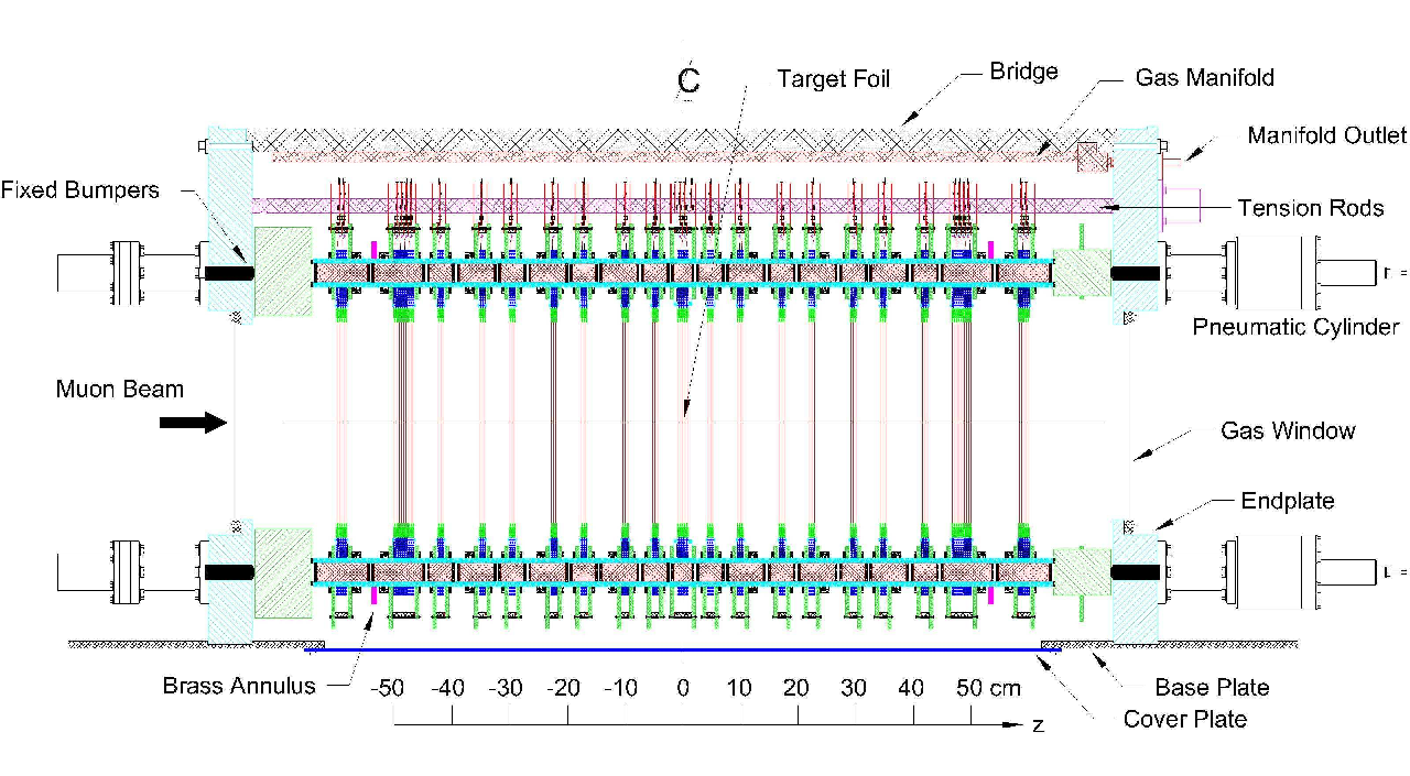
A side view of the stack of wire chambers is shown on Fig. 2.3. The order, as seen by an incoming muon, of the modules is: PCs (4 planes), the “dense stack” (8 DCs), seven modules of “sparse stack” containing a pair of DCs each, the target module. The downstream (after the stopping target) arrangement mirrors the upstream. The DC and PC planes are numbered sequentially, with the numbers increasing along the path of a muon. DC 22 is the last drift chamber and PC 6 is the last proportional chamber before the stopping target.

The target module consists of 4 PC planes. The central cathode foil in this module also serves as the muon stopping target. During the 2002 data taking this target was made from 125 $\mu$ m Mylar, with conductive graphite coating on both sides. (A high purity aluminum stopping target was not available at the time.) Depolarizing interactions in the target rendered 2002 data unsuitable for an improved measurement of $P_{\mu}\xi$ , but the extraction of $\delta$ does not require a precise knowledge of the value of $P_{\mu}$ (page 7.2).

An important advantage of the TWIST detector is the small amount of material in the tracking volume, leading to smaller effects from scattering and energy loss and thus to smaller related uncertainties. The thickness of one pair of DCs is only $1\cdot 10^{-4}$ radiation lengths. Also, the positrons cross only about $25$ mg/cm² of material before entering the tracking volume at the first DC, compared to $240$ mg/cm² before the tracking volume in the previous measurement [27].

A very high mechanical precision has been achieved in the production of the detector. The positions of the planes in the Z direction (along the beam) are defined by precise Sitall ceramic spacers with a negligible coefficient of thermal expansion. The cumulative error on the Z position is less than 50 $\mu$ m over the whole length of the detector [52]. The positions of wires within each plane are accurate to a few microns, see Fig. 2.4. The relative alignment of different wire planes within the detector has been accomplished using 120 MeV/c pion tracks taken with the spectrometer magnet off. The precision of this alignment is 5 $\mu$ m (translations) and 0.01 degrees (rotations) [52].

2.2.2 Electronics and DAQ

A 195 $\mu$ m thick scintillator mounted between the beam pipe and the upstream end of the TWIST detector is used to provide a trigger signal during physics data taking. The scintillator is read out by two PMTs and the trigger condition is a coincidence of the two signals. The thinness of the scintillator makes the system less sensitive to beam positrons, while muons, which have a higher density of energy loss at this momentum, produce a strong signal. An essential feature of the trigger is that it is unbiased: since the decay positron is not used by the trigger system, the trigger efficiency is not correlated with the muon decay parameters.

An electric signal from a DC or PC wire is fed to a pre-amplifier mounted inside the wire chamber module. The output of the pre-amplifier is connected to a post-amplifier/discriminator in a CAMAC crate outside of the detector. The discriminator circuit provides a time over threshold signal, which is recorded by a multihit TDC with 0.5 ns time resolution. Upon receiving a trigger signal the TDC analyzes its internal buffer, and any activity from 6 $\mu$ s before to 10 $\mu$ s after the scintillator hit is read out via FASTBUS by a PowerPC. Time of the leading edge, as well as the width (time over threshold) of the signal are recorded for each of up to 8 hits per wire. Data are sent through an Ethernet connection to a dual 1GHz Pentium Linux computer running a MIDAS [55] based data acquisition system [56], which writes them to a disk buffer, then to SDLT tapes.

The gas gain of the drift chambers combined with the electronic amplification leads to an effective threshold of 1.6 electrons collected from a track to produce a hit [52]. The wire chambers operated at about 99.95% efficiency [52], without a single dead or noisy channel during the 2002 data taking.

In addition to the TDC data, the DAQ logs hundreds of “slow control” variables. They include voltages and currents for individual wire planes, gas flows through the chambers, proton beam current, temperatures at numerous locations in the TWIST detector, NMR measured magnetic fields of the spectrometer and beamline magnets, currents of the beam line magnets, atmospheric pressure, etc.

2.2.3 Spectrometer magnet

The stack of wire chambers is placed inside of a 2 T superconducting solenoid. The solenoid, together with the outside steel yoke, produces highly uniform magnetic field in the tracking volume. The $B_{z}$ component of the field was mapped, Fig. 2.5 shows representative curves from the measurements.

An OPERA-3d [58] simulation model was tuned to the measured $B_{z}$ . The OPERA-3d simulation produces the complete $\vec{B}(\vec{\vphantom{B}r})$ field (as opposed to simply $B_{z}(\vec{r})$ ) that is used by TWIST Monte-Carlo and track reconstruction software. The simulated map reproduces the measured $B_{z}$ to better than 3 Gauss in the tracking region, giving the relative accuracy of $1.5\times 10^{-4}$ .

2.2.4 Beam degraders

To center the distribution of muon stopping position in the target, there is the possibility to fine tune the amount of material in the path of muons. This capability is provided by a gas degrader, a 21.67 cm long volume installed between the vacuum window of the beam pipe and the trigger scintillator. The gas degrader contains a He/CO₂ mixture. The fraction of CO₂ can be varied from 0% to 100%, affecting energy loss of muons in the degrader and their final stopping position.

It is also possible to install a plastic film in the path of muons. It was used to shift the stopping distribution to the upstream end of the stack of wire chambers to acquire the Monte-Carlo verification data (chapter 4).

Chapter 3 TWIST data

With a quasi-continuous beam from the TRIUMF cyclotron, the definition of a “data run” is arbitrary. In TWIST the DAQ was usually instructed to split data into files of about 1.9 GB each. One such file is a “data run”. A typical run contains about $8.5\times 10^{5}$ data events (triggers), and was acquired in about 7 minutes for nominal surface muon beam. Data quality was monitored on per-run basis, and, if a problem was detected, a complete run was excluded from the analysis.

A “data set” was defined as the amount of data required to achieve a statistical precision of ${}\sim 10^{-3}$ on the muon decay parameters. While acquiring a data set, all controllable running conditions were kept unchanged. (However variations in e.g. atmospheric pressure could still introduce differences between runs within a data set.) Set A became significantly smaller than other sets because of an off-line rejection of bad runs. Table 3.1 summarizes data sets used for the extraction of $\delta$ and systematic studies. Note that set A has much lower statistics than other data sets. This is why set B was used in this work to quote typical numbers or show example plots.

Set name	Dates	Number of runs	Fiducial events, millions	Comment
A	Oct 8–9	165	7.9	nominal
B	Nov 21–23	318	15.9	nominal
1.96 T	Dec 2–4	338	16.5	1.96 T spectrometer field
2.04 T	Dec 7–9	240	12.7	2.04 T spectrometer field
Cloud	Nov 6–28	561	12.4	Cloud muon beam
DS Al	Nov 29–30	160	7.7	Outside materials systematic
Slightly Upstream	Oct 5–8	307	7.3	Stopping location systematic
Low rate	Oct 13–20	338	17.9	Beam intensity systematic
High rate	Oct 11–13	341	14.1	Beam intensity systematic
B2 ${}+{}$ 10G	Oct 20–21	348	15.4	Channel magnets systematic

Table 3.1: Data sets mentioned in the thesis. Fiducial region is defined in chapter 5.

All dates are in 2002.

Chapter 4 Monte-Carlo simulation

TWIST uses a very detailed Monte-Carlo simulation program (MC), which is based on the GEANT [59] package. It produced digitized output in the same format as the DAQ, except that additional MC-specific information may be included. Production of a large amount of Monte-Carlo events, matching TWIST data statistics (chapter 3), was made possible by the use of WestGrid computing facility [60].

The geometrical description of the detector contains all the components of the hardware with which a muon or a decay positron could possibly interact. Each individual wire of the wire chambers is implemented in the software. The wire planes are offset and rotated to their as-measured positions. A map of the magnetic field (sections 2.2.3), which extends to the outside of the yoke, is used to propagate charged particles in the simulation.

The initial kinematics of an event contains a muon, and possibly other muons and/or beam positrons. The probability of having the pile-up particles is determined by the specified muon and beam positron rates. The positions and directions of flight of the muons are sampled from experimentally measured distributions $\{x,dx/dz\}$ and $\{y,dy/dz\}$ and reproduce the observed position-angle correlations. The beam particles, muons and positrons, are started outside of the yoke, and GEANT tracking propagates them through the fringe field of the spectrometer magnet into the TWIST detector.

In the TWIST Monte-Carlo, unlike the standard GEANT3, the direction of the muon spin is also tracked in the magnetic field. The initial spin direction is defined as antiparallel to the muon momentum. Depolarizing interactions of the stopped muons are simulated as a step function followed by an exponential relaxation. Setting the initial polarization to $-0.935$ and the time constant to $5.8\cdot 10^{-5}$ s [61] reproduces the behavior of $P_{\mu}(t)$ in data as it is observed for $t>1$ $\mu$ s (this time limit is discussed in chapter 5). A mismatch in polarization between data and Monte-Carlo would not bias the value of $\delta$ in the analysis, but a large difference in the average $P_{\mu}$ could require generating larger “derivative” (chapter 7) samples to achieve the same statistical precision.

The energy loss of a muon is simulated by GEANT, and determines the stopping position of the particle. The simulation of the muon stopping process has been validated using special data runs with muons stopping in the middle of the upstream part of the chamber stack. Because each of the chamber modules is much thinner than the stopping target, the muon stopping distribution in these runs spreads out over several wire chambers, and the distribution of the last (the most downstream) wire plane hit by muon can be used to observe the shape of the stopping distribution. It has been shown [62] that the simulation matches the shape of the stopping distribution well, but a constant offset equivalent to an about 86 $\mu$ m of additional plastic (Mylar) is required in Monte-Carlo to match the mean stopping position of the muons. The peak of the stopping distribution within the target is not directly observable in data, but the tails of the distribution are still accessible through the last plane hit information. The following procedure was used to determine the setting of the gas degrader for the nominal data taking. A histogram of the last muon hit from Monte-Carlo, with the stopping distribution centered in the target, was compared with similar histograms from data for different settings of the gas degrader. The setting corresponding to the best match to the Monte-Carlo distribution was used for the data taking. All nominal Monte-Carlo sets were generated with the muon stopping distribution centered in the target. The energy calibration procedure (chapter 6) compensates for any remaining differences in the average muon stopping position.

A muon decay subroutine returns the energy and angle of the decay positron with respect to the muon spin as dictated by the Michel parameters input. The theoretical decay spectrum includes full ${\cal{O}}(\alpha)$ radiative corrections with exact electron mass dependence, as well as leading and next-to-leading logarithmic terms of ${\cal{O}}(\alpha^{2})$ , leading logarithmic terms of ${\cal{O}}(\alpha^{3})$ , corrections for soft pairs, virtual pairs, and an ad-hoc exponentiation [17, 18, 19, 20, 21]. The actual implementation of the muon decay spectrum is separated from the rest of the Monte-Carlo code to make possible a blind analysis, as is explained in section 7.4.

The wire chamber response is simulated by randomly creating ionization clusters along the path of a charged particle when it crosses a drift cell, calculating the drift time of each cluster to the wire, and simulating the overlap of different clusters to produce an above-the-threshold signal. The obtained time of the signal is smeared to simulate electronics effects. The parameters of the method are derived from a detailed GARFIELD [63] simulation study [64], and the “electronics” smearing is tuned to TWIST data. The critical piece of information affecting the accuracy of track reconstruction (chapter 5) is the time of the leading edge of DC chamber signals. A good match of the simulated distribution to TWIST data has been demonstrated [65].

Full GEANT physics interactions are enabled, so such processes as creation of delta-electrons, or conversion of a bremsstrahlung photon into an electron-positron pair, may create additional hits on the detector wires.

Interactions of decay positrons in detector materials distort the reconstructed spectrum and can lead to biases in the values of the measured decay parameters. TWIST relies on Monte-Carlo to compensate for these effects (chapter 7). Knowing the accuracy of the simulation of the interactions is important to determine the corresponding systematic uncertainty (chapter 8). To verify a claim that in GEANT3

the cross-sections of the electromagnetic processes are well reproduced (within a few percent) from 10 keV up to 100 GeV, both for light (low Z) and for heavy materials

([59], section PHYS001), data runs with muons stopped in the upstream end of the detector have been taken. In these runs a decay positron emitted in the downstream direction crosses the whole spectrometer. The upstream and downstream halves of the detector can be used as two independent devices to measure the momentum and angle of the positron before and after the central target, thus allowing an extraction of the energy loss and angular scattering distributions from data. These distributions can be compared with similar distributions obtained from a corresponding Monte-Carlo simulation. The Monte-Carlo validation data were taken in 2003, with a high purity aluminum stopping target of a known thickness. Thus the validation, unlike the final result, is not affected by the uncertainty in the thickness of the graphite coating on the Mylar stopping target used for the main 2002 data sets.

Fig. 4.1 shows an overlay of the momentum loss distributions for data and Monte-Carlo. There $\Delta{p}=p_{\text{downstream}}-p_{\text{upstream}}$ is the difference between the positron momenta reconstructed by the two halves of the detector. In TWIST geometry momentum loss of a positron is proportional to $1/|\cos(\theta)|$ (see chapter 6); a factor of $|\cos(\theta)|$ is used in the study to compensate for a possible difference in the angular distributions of the emitted positrons between data and Monte-Carlo while comparing the momentum losses. The difference between the data and the simulation does not exceed 5% for both the average losses, and the widths of the distributions. To separately look at “hard” processes, an arbitrary bound of 1 MeV/c was defined. The tails of the distributions shown on Fig. 4.1 were integrated from $-\infty$ to $-1.12$ MeV/c (i.e. to 1 MeV/c below the average). The discrepancy in the fraction of such “hard scatter” events was found to be 14%. Therefore the numbers we used to estimate a systematic uncertainty due to the quality of GEANT simulation of positron interactions are 14% for hard interactions, and 5% for intermediate and soft interactions.

The distribution of $\Delta\theta=\theta_{\text{downstream}}-\theta_{\text{upstream}}$ is shown on Fig. 4.2. The width of the distributions agrees to about 1%, but there is a noticeable shift in the mean value of $\Delta{\theta}$ . The interpretation of the mean value of this distribution is complicated. Since there is more phase space at higher angles due to the $\sin\theta$ factor, a naive expectation is to observe a small positive shift in $\Delta\theta$ . This has been confirmed by a Monte-Carlo study [66], which demonstrated a ${}\sim 1$ mrad positive bias. An effect of a non-uniformity of the magnetic field is negligible [66]. However the distribution of the reconstructed $\Delta\theta$ has a negative mean for both data and Monte-Carlo. Thus is should be attributed to biases in the track reconstruction, which affect the two halves of a track in a different way. At least two causes for such biases are known. In the GEANT validation studies positrons originate in PC 4, and no information from PC 1–3 is available for pattern recognition (chapter 5) for the upstream part of a track, but full information is available for the downstream part. Also, the track fitting always assumes that a positron originates in the stopping target to determine the sign of a time-of-flight correction to drift chamber hits. Therefore the correction was applied with the wrong sign for the upstream parts, and with the correct sign for the downstream parts of tracks in the validation study. Such biases are common for the data and the simulation, and may shift the distributions to negative $\Delta\theta$ . A possible explanation for the difference in the central values between data Monte-Carlo is a misalignment of the detector to the magnetic field. Chapter 8 evaluates a systematic uncertainty associated with such a misalignment.

It has to be noticed, that the widths of the distributions on Fig. 4.1 and Fig. 4.2 do not represent TWIST resolutions. The lack of information from PC1–3, and the wrong time-of-flight correction mentioned above worsen the tracking quality. Moreover, a positron in these studies goes through twice as much material as a positron from a muon stopped in the target. Also, a track is reconstructed in the two halves of the detector, so random fitting errors contribute twice.

Chapter 5 Spectrum reconstruction

The primary purpose of the spectrum reconstruction is to produce a 2-dimensional spectrum of decay positrons in momentum and angle using information available from the TWIST detector.

Real and simulated data are analyzed by the same reconstruction code in essentially the same way. The only non-trivial difference in treating the two cases is the crosstalk removal, which is discussed below. Technically the analysis was done in two stages. The first stage, required a large amount of computations and was performed at WestGrid [60]. It consisted of the following steps:

Crosstalk removal.: A hit on a wire may induce a signal in a different channel through electronics crosstalk. Most of crosstalk in TWIST is induced by highly ionizing muons, therefore it does not affect decay positrons a microsecond later.

The effect has been studied in detail in the hardware by pulsing a channel and observing the crosstalk signal on an oscilloscope. Crosstalk signals have characteristics allowing for their identification and removal by software [67]: there is a 5–65 ns delay from the generating pulse, and the width of a crosstalk signal is much smaller than the width of a real signal.

An algorithm utilizing these characteristics removes crosstalk hits from real data events before any other analysis is done. Because crosstalk is not simulated by TWIST Monte-Carlo, and also because the width of chamber signals in the simulation is not tuned to data, this algorithm is not invoked on Monte-Carlo events.
Windowing.: Chamber hits are grouped in time. Different groups correspond to tracks from different particles.
Classification.: For each time window, characteristics of its chamber hits are used to guess what process has occurred there [68]. For example, a decay positron hits wire chambers in only one half of the detector, while a beam positron crosses the whole detector. Based on the number and type of time windows in an event, and the times of different windows, a classification code is assigned to the event [68].
Pattern recognition.: A cluster of consecutive wires hit in a plane determines only one transverse coordinate of a passing track. Information from an orthogonal pair of wire planes can be used to determine a “space point” on the track.

For a time window, the pattern recognition uses space points formed by the hits belonging to the window to find parameters of possible helical tracks passing through the points. It uses a combinatorial technique [69, 70] and can find more than one track per window.

A feature of the arrangement of the wire chamber modules in the detector, which can be seen on Fig. 2.3, is that the distances between the corresponding planes of different pairs form a pattern: 5.2 cm, 7.2 cm, 5.2 cm, 7.2 cm, 5.2 cm, 7.2 cm, with only two independent distances, for the 7 modules closest to the stopping target on either side. That means that a helix with the wavelength $L=5.2+7.2=12.4$ cm has only two distinct measurements of its transverse position, so its radius can not be reconstructed using the space points [71, 72]. (In a projection along the detector axis, the 7 space points collapse into only 2 points on the circle—projection of the helix.)

The “dense stacks” of wire planes at the outer edges of the detector, along with information from PC chambers, help to resolve the ambiguity. However the worsening of the quality of reconstruction of such tracks still prompted the introduction of a fiducial cut on $p_{z}$ , described below, to stay away from the “magic wavelength” zone.
Wire center fits.: Tracks are fit to the positions of hit wires in a time window. The “narrow windows” technique [73] is used. To account for multiple scattering, kinks at the positions of sparse stack chamber modules are allowed [74]. The magnetic field map (section 2.2.3) is used. The resulting fit has sufficient precision to resolve most left-right ambiguities.
Track fitting: The parameters of the tracks are refined using drift time information. The necessary space-time relations are obtained from GARFIELD. Kinks and magnetic field map are used.

No cuts on events were imposed at the first stage, and a summary of each event was written out in a “ROOT tree” format [75]. The output data were subsequently analyzed to select events and tracks to be used in the final spectrum. The following cuts, illustrated on Fig. 5.1, were used.

TCAP.: This is a cut on the time of flight of the trigger particle through the M13 beam line. It selects muons from stopped pions that decayed in between the proton pulses from the cyclotron, and rejects “cloud” muons (section 2.1). The purpose of the cut is to improve muon polarization. It also rejects triggers from beam pions and prompt positrons.

The time of flight cut is only applied to data events. The Monte-Carlo does not simulate the 43 ns time structure of the beam, and is instead produced using measured parameters of the surface muon beam with the TCAP cut applied.
Event Type.: This cut uses the event classification code, and is a combination of several requirements. The event must be triggered by a muon, and not a beam positron. There must be only one identified muon. A unique decay time window must be identified.

The decay must happen at least 1.05 $\mu$ s after the trigger to ensure that DC hits with the longest drift time ${}\sim 1$ $\mu$ s from the muon do not affect reconstruction of the decay positron. Since the muon life time is about 2.2 $\mu$ s, this requirement alone rejects 38% of events.

Pile-up beam positrons are allowed, but they must be well separated in time (at least 1.05 $\mu$ s) from both the muon and the decay positron to avoid an overlap of DC hits. Events with DC overlap constitute another major fraction of all events rejected by the Event Type cut. It is important to note that rejection of DC overlap events does not introduce a bias in the spectrum, because the probability of an overlap does not depend on the momentum and angle of the decay positron.

On the other hand, beam particles within ${}\sim 100$ ns of the decay can not be reliably separated by the classification code from such processes as creation of delta-electrons or backscattering of the decay positron. Therefore all such “PC overlap” events are kept at this stage.
Muon Z.: Require that the event is consistent with the muon stopped in the central target, i.e. require that the last chamber hit by the muon is PC 6.
Muon radius.: Constrain muon stopping position in the transverse plane to $r<2.5$ cm.
Decay Window Time.: Require the decay to occur before 9 $\mu$ s from the trigger, so that long drift time hits are not cut off by the 10 $\mu$ s DAQ limit.
N tracks: Require at least one track candidate, as defined by the pattern recognition, in the decay window.

All the cuts above are essentially event-level cuts. An event may contain more than one successfully reconstructed track. There are several reasons for multiple tracks to be found. For example, due to a hard scatter a decay track may be split into two helical parts, before and after the scatter, by the pattern recognition. That would lead to two fit tracks for a single decay positron. Or a decay positron may backscatter off material outside, re-enter the tracking volume, and produce a second track, which may cross the whole detector. Such events may be indistinguishable from a decay being overlapped by a beam positron particle. A genuine beam positron overlap is yet another possibility to produce multiple tracks.

The challenge is to identify the “correct” track to be included in the spectrum. It is handled as following [76]. A set of “decay candidate tracks” is created. Initially it consists of all tracks identified in the decay window by the pattern recognition. Then each of the candidates is subject to the cuts below. Failed candidates are eliminated from the set. A corresponding event-level cut is defined as the requirement that the set of decay candidates is not empty after the track cuts.

ierror

Eliminate track candidates that did not produce a successful fit.

startstop

Require that the ends of a fit track are on the “correct side” of the detector, as determined by the classification. I.e. the track begins and ends in the upstream half for upstream decay type events, in the downstream half for downstream decay type events. Tracks that cross the central target are always rejected here.

charge

The direction of the winding of the helix must be consistent with a positive particle that originated in the central target.

pair matches

This piece of code essentially attempts to “glue” pieces of tracks that were split in the reconstruction because of a hard scatter [76].

The cut is done in two stages. First, for each track among the decay candidates, a set of “anti-tracks” is found as described below. An “anti-track” for a decay candidate is a track in the decay window that, if successfully “glued” to the candidate, would indicate that the candidate track should not be used.

Then the closest distance of approach¹¹ 1 The distance used is the shortest distance between two tracks in the transverse plane, not in 3D. (CDA) is calculated between the candidate and each of its anti-tracks. If CDA is less than 0.5 cm for at least one anti-track, the candidate is rejected: probably the anti-track and the candidate track belong to the same particle. The decision is done on purely geometrical grounds: do the two tracks intersect? They can belong to the same particle only if they do.

Selection of anti-tracks

The set of anti-tracks for a decay candidate is found through the following procedure:

1.

Start with all good fits in the decay window, but exclude the decay candidate itself, to form a set of anti-track candidates.
2.

Exclude all tracks which overlap with the decay candidate in Z. If two tracks have hits in the same DC plane, they can’t be from the same particle. (Sharing of DC hits in not allowed in the track fitter. One DC hit could belong to no more than one fit track.)
3.

Exclude all tracks which are in the same half of the detector and farther from the target than the decay candidate. We want to keep the decay candidate because it is closer to the target, and therefore provides more accurate information on the momentum and angle of the positron at the decay point, even if the anti-track belongs to the same particle.

At this point an event is accepted and will produce an entry in the final spectrum. However there is still no guarantee that a unique decay track has been identified. In fact about 0.7% of events still contain more than one decay track candidate, as can be seen on Fig. 5.2. The following algorithm [76] is used to decide among the multiple candidates. These “selects”, unlike cuts, never reject all candidates, but choose one.

dplane to target: Find the DC plane closest to the central target, which is used by a decay candidate. Eliminate all candidates that do not use a hit from that plane, and therefore start farther from the target.
mu-e vertex: The remaining ${}\lesssim 10^{-4}$ fraction of multiple track cases is resolved by the proximity of extrapolation of the positron tracks to the muon stopping position. Since the error on the two muon coordinates is significantly different because of the large scattering near its stopping position, an elliptical metric is used: $R_{\text{ellipse}}=(U_{e}-U_{\mu})^{2}+(V_{e}-V_{\mu})^{2}/\sigma_{vu}^{2}$ , with $\sigma_{vu}=1.7$ found empirically by comparing RMS of muon-positron mismatch in the $U$ and $V$ directions.

The code is guaranteed to select only one decay track per event.

The momentum and $\cos(\theta)$ values of the selected tracks represent an unbinned decay spectrum. This “raw” spectrum was used to perform the energy calibration procedure, described in chapter 6. Then calibration results were applied to the unbinned decay spectrum (chapter 6), and the corrected spectrum was filled into a 2-dimensional histogram in momentum and $\cos(\theta)$ , which was further used to perform a fit and extract values of the muon decay parameters (chapter 7). An example of a reconstructed data spectrum is shown in Fig. 5.3.

The fiducial region used in the extraction of $\delta$ is defined by the following constraints:

$\boldsymbol{p}\boldsymbol{<}\boldsymbol{50}$ MeV/c: The shape of the reconstructed spectrum at the end point is defined by the detector resolution. On the other hand, in the bulk of a smooth spectrum its distortion due to detector resolution is a second order effect. Excluding the end point region from the decay parameter fits (chapter 9) drastically reduces the sensitivity of the result to discrepancies between resolutions for real and simulated data.

Another reason to stay away from the end point is to keep the decay parameter fits statistically independent from the energy calibration fits (chapter 6).
$\boldsymbol{|p_{z}|>13.7}$ MeV/c: This cut eliminates tracks affected by the “magic wavelength” problem, which is discussed above in this chapter.
$\boldsymbol{p_{t}<38.5}$ MeV/c: That requirement, together with the $r<2.5$ cm cut on the muon stopping position, insures that the decay positron track is radially contained within the instrumented region of the detector.
$\boldsymbol{0.50<|\cos\theta|<0.84}$: Events at high angles (small $|\cos(\theta)|$ ) are more affected by multiple scattering and momentum struggling, leading to worse resolution. They are also more difficult to reconstruct.

At small angles, it becomes difficult to determine the wavelength ( $p_{z}$ ) of the tracks. Reconstruction biases observed in this region lead to a deviation of the average energy loss $p_{\text{rec}}-p_{\text{MC}}$ from the $1/|\cos(\theta)|$ behavior required for energy calibration (chapter 6).

The shape of the fiducial region in the momentum and $\cos(\theta)$ plane can be seen in the upper left panel of Figs. 9.1–9.5.

The average resolutions in the fiducial region are: 150 keV (FWHM) for momentum, 0.015 rad (FWHM) for the $\theta$ angle, and 0.01 (FWHM) for $\cos(\theta)$ . Distributions of the differences of reconstructed and Monte-Carlo values for events reconstructed within the fiducial are shown on Fig. 5.4.

Chapter 6 Energy calibration

The momentum of a decay positron measured by TWIST is affected by energy loss in the detector materials. For a muon stopping distribution that is not centered in the target the average momentum shift is different for upstream and downstream decays, introducing an asymmetry in the spectrum. Also the average energy loss may be different in data and the simulation even for a centered stopping distribution. The momentum also scales with the ratio of the “true” magnetic field seen by the particle to the field used by the reconstruction program. The ratio is unity for the Monte-Carlo, but the field map is not a perfect representation of the real field. These effects may lead to different spectrum distortions for real and simulated data, producing a bias in the extracted values of the muon decay parameters. The goal of the energy calibration procedure is to correct the reconstructed spectra to compensate for these differences between the data and the simulation.

The calibration is done on physics data, using the same reconstructed spectrum as for the extraction of the decay parameters. The calibration point is provided by the sharp edge of the muon decay spectrum at the upper kinematic limit. Its position is determined by the muon and the positron masses, and is therefore known.

The planar geometry of the TWIST spectrometer leads to an exact $1/|\cos(\theta)|$ dependence of the amount of material traversed by a decay positron [50]. This dependence is obvious for the flat stopping target, cathode foils, and the gas layers. For the cylindrical wires, that dependence still applies on average, because the probability of hitting a wire changes as $1/|\cos(\theta)|$ . In the 15–53 MeV/c TWIST range of momenta, this translates into a linear dependence of the average energy loss of the positron on $1/|\cos(\theta)|$ . That known dependence provides a way to disentangle the effects of the magnetic field scale, which is angle-independent, and the energy loss. The position of the spectrum end point as a function of angle is given by

p^{\text{raw}}_{\text{edge}}(\theta)=\left(1+\frac{{\beta}}{p_{0}}\right)\left(p_{0}-\frac{{\alpha}}{|\cos(\theta)|}\right).

(6.1)

Here $p^{\text{raw}}_{\text{edge}}(\theta)$ is the end point position of the “raw” reconstructed spectrum, $p_{0}\approx 52.828\text{~MeV}$ is the kinematic spectrum limit, and the constants $\alpha$ and $\beta$ describe the momentum loss and the field scale mismatch, respectively. To accommodate a non-centered muon stopping distribution, the calibration procedure allows for different energy loss parameters in the upstream and the downstream parts of the detector, $\alpha=\alpha_{u}$ or $\alpha=\alpha_{d}$ . The difference of the upstream and downstream energy losses $\alpha_{\text{diff}}=\alpha_{u}-\alpha_{d}$ is proportional to an offset of the muon stopping distribution from the centered position, while the sum $\alpha_{\text{sum}}=\alpha_{u}+\alpha_{d}$ does not depend on the muon stopping position and is a measure of an effective thickness of the detector.

A determination of the calibration parameters $\beta$ , $\alpha_{u}$ , $\alpha_{d}$ is not trivial. The challenge is to determine the end point position, $p^{\text{raw}}_{\text{edge}}(\theta)$ , on reconstructed data, where the sharp edge of the theoretical spectrum is smeared by the detector resolution. A model function describing the spectrum shape at the end point is needed. This complicated shape is a convolution of the muon decay spectrum and the detector resolution, and a model function can not be expected to perfectly describe the data distribution. Therefore the result of a fit depends on the range of momenta used. An objective procedure establishing the range must be developed. Since the bias of a fit depends on the relative position of the fit range with respect to the end point, that procedure should be adaptive and produce the same relative position for different absolute positions of the end point in the input data. It also has to be noticed that fitting in the end point region by definition involves transition from high to low per bin statistics, and care must be exercised in handling the statistical issues properly.

A straightforward approach of fitting $p^{\text{raw}}_{\text{edge}}(\theta)$ independently for different angles, with an adaptive choice of fit range, and then applying Eq. (6.1) to fit a straight line through the resulting points, has been tried [77, 78]. Different end point model functions were used, some including the effects of radiative corrections on the muon decay spectrum [77]. An important result of these studies is a demonstration that the end point indeed has a $1/|\cos(\theta)|$ dependence. However to stabilize the independent end point fits, especially for small downstream angles where the statistics is low, a large range of momenta ${}\approx 2$ MeV/c needs to be used. It is more difficult to find a model function describing the data in a large range. Another issue is that the shape of the data distribution becomes sensitive to the values of the muon decay parameters if a large range of momenta is looked at, which is an undesirable effect. Also, there is no single goodness of fit criteria in this approach. The goodness of the final straight line fit does not include any information about goodness of the individual end point fits.

To overcome these issues, a fitting procedure that uses a global fit to the 2-dimensional momentum and $\cos(\theta)$ reconstructed distribution has been developed [79]. The model function is constructed as following. The momentum dependence is given by a convolution of a “slope and a step” shape

a\,(1+by)\,\Theta(y),\quad\text{where}\quad y=p-p_{\text{edge}}

(6.2)

with a Gaussian, illustrated on Fig. 6.1. Here $\Theta(y)$ is the Heaviside step function. There are 4 parameters $a$ , $b$ , $p_{\text{edge}}$ , which defines the position of the end point, and the Gaussian $\sigma$ . The explicit form of the end point model is

\frac{1}{2}(a+by)\erfc(\frac{y}{\sqrt{2}\,\sigma)})-\frac{b\sigma}{\sqrt{2\pi}}\exp(-\frac{y^{2}}{2\sigma^{2}}).

(6.3)

This one-dimensional function is used to describe the momentum dependence of the spectrum for a fixed angle $\theta$ . To obtain a 2-dimensional function, a dependence of the parameters $a$ , $b$ , $p_{\text{edge}}$ and $\sigma$ on $\theta$ is introduced. For $p_{\text{edge}}$ , the expected linear in $1/|\cos(\theta)|$ behavior from Eq. (6.1) is used, with different momentum loss parameters $\alpha_{u}$ and $\alpha_{d}$ but common field scale $\beta$ in the upstream and the downstream:

	$\displaystyle p^{\text{raw}}_{\text{edge}}(\theta)$	$\displaystyle=\left(1+\frac{{\beta}}{p_{0}}\right)\left(p_{0}-\frac{\alpha_{u}\Theta(-\cos(\theta))+\alpha_{d}\Theta(\cos(\theta))}{\|\cos(\theta)\|}\right).$	(6.4)
The muon decay spectrum is linear in $\cos(\theta)$ , therefore a linear parameterization
	$\displaystyle a(\theta)$	$\displaystyle=a_{0}+a_{1}\cos(\theta)$	(6.5)
is used for the normalization. For $\sigma$ and $b$ , suitable parametrizations were found empirically by fitting Eq. (6.3) to the data distribution independently for different angular bins, and observing the behavior of the fitted parameters as functions of angle. That resulted into the following choice:
	$\displaystyle b(\theta)$	$\displaystyle=b_{0}+b_{1}\cos(\theta).$	(6.6)
	$\displaystyle\sigma(\theta)$	$\displaystyle=\frac{\sigma_{0}}{\|\sin(\theta)\|},$	(6.7)

Equations (6.3)–(6.7) completely define the shape of the fitting function. They contain 8 parameters: $\beta$ , $\alpha_{u}$ , $\alpha_{d}$ , $a_{0}$ , $a_{1}$ , $b_{0}$ , $b_{1}$ , $\sigma_{0}$ , that are determined from a fit to a reconstructed spectrum. Fig. 6.2 shows an energy calibration fit to data for several angles.

The fit is done by minimizing $-2\ln\lambda$ , where $\lambda$ is the Poisson likelihood ratio [80]:

-2\ln\lambda=2\sum_{i=1}^{N}\left[f_{i}-n_{i}+n_{i}\ln\frac{n_{i}}{f_{i}}\right].

(6.8)

In (6.8) the summation runs over the bins of the histogram in the fit range, $n_{i}$ is the number of entries in a bin, and $f_{i}$ is the expectation value for $n_{i}$ computed using Eqs. (6.3)–(6.7). The advantage of the binned likelihood statistics $-2\ln\lambda$ is that it can be used not only to perform the fitting, but also to easily estimate a goodness of the resulting fit [80]. In the large sample limit the minimum value of $-2\ln\lambda$ is distributed as $\chi^{2}$ .

As is mentioned above, for a fixed angle the same momentum fit range relative to the end point must be selected, so that no biases between data and Monte-Carlo are introduced due to different absolute positions of end points. A series of tests, described in Appendix Appendix B
Optimization of fit range
for the energy calibration procedure, led to the following choice:

p_{\text{edge}}(\theta)-0.75\text{~MeV/c}<p<p_{\text{edge}}(\theta)+0.5\sigma(\theta).

(6.9)

The fit is done iteratively. It uses its current estimate of $p_{\text{edge}}(\theta)$ to fix the fit range for the next iteration. There is no explicit limit on the number of iterations. Instead each new 2-dimensional fit region $\Omega_{k}$ is compared with all previously seen regions $\Omega_{1},\ldots,\Omega_{k-1}$ . The stopping condition is $\Omega_{k}=\Omega_{k-l}$ . Because a binned fit is used, a rounding to histogram bin boundaries ensures that the number of possible fit regions is finite, so the fit always converges. In practice it usually takes ${}\lesssim 10$ iterations. It is common to have $l>1$ , in that case the average value of $\beta$ over iterations $k-l+1,\ldots,k$ is computed, and the iteration with $\beta$ closest to the average is chosen as the final result. This is an arbitrary procedure, but the spread of the results over the regions of the “convergence cycle” is always much smaller than the statistical error of the fit.

Table 6.1 shows results of energy calibration fits for data sets and corresponding Monte-Carlo sets used in the extraction of $\delta$ . A systematic difference in the momentum resolution parameter $\sigma_{0}$ at the end point is apparent from the numbers.

Spectrum	$\beta$	$\alpha_{u}$	$\alpha_{d}$	$\sigma_{0}$
Set A	$-5.4\pm 6.2$	$67.7\pm 5.4$	$56.9\pm 5.4$	$76.0\pm 1.7$
Set B	$3.6\pm 5.5$	$74.0\pm 3.8$	$60.2\pm 3.8$	$74.1\pm 1.2$
1.96 T	$9.0\pm 5.4$	$79.0\pm 3.8$	$71.3\pm 3.8$	$76.8\pm 1.2$
2.04 T	$8.0\pm 6.0$	$75.9\pm 4.2$	$64.8\pm 4.2$	$73.3\pm 1.3$
MC A	$-41.2\pm 4.5$	$61.4\pm 3.1$	$57.8\pm 3.1$	$69.3\pm 0.9$
MC B	$-42.0\pm 4.5$	$60.3\pm 3.1$	$57.3\pm 3.1$	$69.1\pm 1.0$
MC 1.96 T	$-7.1\pm 4.5$	$58.4\pm 3.2$	$56.0\pm 3.1$	$69.7\pm 1.0$
MC 2.04 T	$-9.0\pm 4.5$	$56.8\pm 3.1$	$55.4\pm 3.1$	$68.7\pm 0.9$

Table 6.1: Energy calibration results. All parameters are in keV/c. The large deviations in

\beta

for two of the Monte-Carlos are because of a mistake in setting the field scale in MC production. The energy calibration procedure corrects for this mistake.

This discrepancy may arise for multiple reasons. For example, the spectrum reconstruction uses the same drift chamber space-time relations for data and Monte-Carlo. These relations may be slightly different in the real detector, but the simulation uses exactly the same drift tables as the reconstruction to generate Monte-Carlo events. Therefore the reconstruction of Monte-Carlo can be expected to perform better. This holds true for all other calibrations, such as alignment corrections, electronic timing offsets T0, etc. The GEANT handling of positron interactions in detector materials may also contribute to the effect. All the calibrations are counted as sources of their corresponding systematic uncertainties, as well as an imperfection of the GEANT simulation, chapter 8. However an effect of the momentum resolution discrepancy on the final result, regardless of its cause, has been estimated and included in the final estimate of systematic uncertainty, chapter 8.

Typical correlation coefficients among fit parameters are shown in Table 6.2. Since the parameters of interest $\beta$ , $\alpha_{u}$ and $\alpha_{d}$ are highly correlated, their correlation must be taken into account while estimating a systematic uncertainty of the result due to energy calibration.

\begin{array}[]{l|d{2.2}d{2.2}d{2.2}d{2.2}d{2.2}d{2.2}d{2.2}}&\lx@intercol\hfil\alpha_{u}\hfil\lx@intercol&\lx@intercol\hfil\alpha_{d}\hfil\lx@intercol&\lx@intercol\hfil\sigma_{0}\hfil\lx@intercol&\lx@intercol\hfil a_{0}\hfil\lx@intercol&\lx@intercol\hfil a_{1}\hfil\lx@intercol&\lx@intercol\hfil b_{0}\hfil\lx@intercol&\lx@intercol\hfil b_{1}\hfil\lx@intercol\\ \hline\cr\beta&0.98$&0.93$&-0.14$&-0.27$&-0.09$&-0.24$&0.14$\\ \alpha_{u}&$&0.92$&-0.06$&-0.12$&-0.14$&-0.11$&0.00$\\ \alpha_{d}&$&$&-0.06$&-0.12$&0.13$&-0.10$&0.16$\\ \sigma_{0}&$&$&$&0.65$&-0.01$&0.58$&-0.45$\\ a_{0}&$&$&$&$&0.03$&0.96$&-0.72$\\ a_{1}&$&$&$&$&$&0.02$&0.59$\\ b_{0}&$&$&$&$&$&$&-0.75$\end{array}

Table 6.2: Correlation coefficients for energy calibration fit to set B.

An energy calibrated decay spectrum is obtained from the corresponding “raw” spectrum by recomputing the reconstructed momentum for every event:

p^{\text{ec}}=\frac{p^{\text{raw}}}{1+\beta/p_{0}}+\frac{\alpha}{|\cos(\theta)|}

(6.10)

The momentum is scaled by the magnetic field scale, and corrected for the energy loss. $\alpha=\alpha_{u}$ for upstream decays, $\alpha_{d}$ for downstream. $p_{0}$ is defined after Eq. (6.1). This calibration procedure brings the end point of the calibrated spectrum to its “theoretical” value, $p_{\text{edge}}(\theta)=p_{0}$ . Checks by running energy calibration fits on calibrated (instead of raw) spectra were done. As expected resulting $\beta$ , $\alpha_{u}$ , and $\alpha_{d}$ were consistent with zero.

Chapter 7 Method for extraction of the decay parameters

A reconstructed spectrum differs from a theoretical one because of finite experimental resolution and because the interaction of the decay positrons with detector materials changes the energy and angle of the particles.

Consider a parametrized theoretical probability distribution function $f_{\text{theor}}(x^{\prime};\lambda)$ , $x^{\prime}\in\Omega_{0}$ , where $\lambda$ are the parameters of the theory, and the $x^{\prime}$ are the kinematic variables of interest. The probability $K(x,x^{\prime})\,dx$ of reconstructing an event that occurred at $x^{\prime}$ in a volume $dx$ around some point $x$ defines the response function $K$ , which describes the combined effect of the detector and the reconstruction. The reconstructed spectrum $f_{\text{rec}}(x;\lambda)$ can be written as

f_{\text{rec}}(x;\lambda)=b(x)+\int_{\Omega_{0}}K(x,x^{\prime})\,f_{\text{theor}}(x^{\prime};\lambda)\,dx^{\prime},

(7.1)

where $b(x)$ is the background term.

Several approaches can be used to deduce the theory parameters $\lambda$ from a measured spectrum, $f_{\text{rec}}$ . One can try to solve (7.1) for $f_{\text{theor}}$ . Deconvolution methods are available [81], and were used by some experiments (e.g. [82]). However they are not practical for TWIST where since $x=\{p,\cos(\theta))\}$ , $K$ is a function of 4 variables $p$ , $\cos(\theta)$ , $p^{\prime}$ , $\cos(\theta^{\prime})$ . It is difficult to estimate a 4-dimensional function accurately from Monte-Carlo. In addition, a general feature of unfolding methods is a need for a regularization parameter, which biases the result.

Another approach is to approximate (7.1) by an analytic expression, and use the resulting $f_{\text{rec}}(x;\lambda)$ to fit the data. Some terms in the approximate expression usually need to be determined from simulations. This method is used by e.g. [27]. It would be difficult to find a suitable expression for the high precision representation of the spectrum required by TWIST.

The rest of this chapter describes yet another technique, which was used by TWIST. The idea is to parametrize the reconstructed spectrum in terms of $\lambda$ , and use that parameterization to fit the data. The method is similar to the one described in [83]. The TWIST method differs from [83] in the fact that we fit only spectrum shape parameters, but not the absolute normalization.

7.1 The fitting method

Appendix Appendix C
The spectrum expansion derives an expansion of a reconstructed spectrum in the general case. In TWIST background contamination is ${}\lesssim 10^{-4}$ [84]. Moreover, the primary background is simulated by TWIST Monte-Carlo. This means that there is a cancellation of the corresponding spectrum distortion, and the effect is negligible at the $10^{-3}$ level of precision. Therefore Eq. (C.22) can be simplified to

n_{i}(\lambda+\Delta\lambda)=\left[1-\sum_{\alpha=1}^{m}\Delta\lambda_{\alpha}\,{\cal E}^{-1}\nu^{\alpha}\right]n_{i}(\lambda)+\sum_{\alpha=1}^{m}\Delta\lambda_{\alpha}\>{\cal E}^{-1}\nu_{i}^{\alpha}

(7.2)

where we also have omitted the ${\cal{O}}(\Delta\lambda^{2})$ term. Here $n_{i}(\lambda+\Delta\lambda)$ are bin contents of a normalized data histogram, $n_{i}(\lambda)$ are corresponding “base” Monte-Carlo values, $\nu_{i}^{\alpha}$ are bins of a Monte-Carlo histogram for a “derivative” spectrum corresponding to $\lambda^{\alpha}$ , and ${\cal E}^{-1}$ is a constant that can be determined from simulation. See Appendix Appendix C
The spectrum expansion for details.

To extract values of the muon decay parameters, we minimize the

\chi^{2}=\sum_{\Omega}\frac{(n_{i}^{\text{Data}}-n_{i}^{\text{MC}})^{2}}{\sigma_{i}^{2}}

(7.3)

where $n_{i}^{\text{Data}}$ are the normalized contents of a data spectrum histogram, and $n_{i}^{\text{MC}}$ are calculated according to (7.2) using Monte-Carlo ‘‘base’’ and ‘‘derivative’’ spectra. The errors are assumed to be Gaussian, since the available statistics are sufficiently high¹¹ 1 The statistics are always high for “data” and “base” spectra. Some derivative functions cross zero in the fiducial, and around the crossings the count of events in a bin for the corresponding derivative may be small. However the total error on the bin is dominated by “data” and “base” distributions, so the smallness of a derivative count has no importance. . The error on the content of bin $i$ of an input histogram is taken as the square root of the number of entries in that bin, then the errors on different MC histograms are combined following (7.2), and $\sigma_{i}^{2}$ is calculated as $\sigma_{i}^{2}=(\sigma^{\text{Data}}_{i})^{2}+(\sigma^{\text{MC}}_{i})^{2}$ .

The technique of extracting muon decay parameters through expansion (7.2) takes into account effects of the detector (such as interactions of decay positrons in the detector materials) and of the reconstruction (such as possible biases and inefficiencies of the track fitting). No further corrections to the fit result are required.

An important advantage of the method is that effects of the reconstruction cancel exactly, since the same software is used to process real data and Monte-Carlo. This fact allows for attributing all systematic effects to deficiencies of the simulation. (Indeed, a perfect simulation would be reconstructed exactly as data by any reconstruction software.) On the other hand, the TWIST detector is very thin, so that the spectrum distortions it causes are small in the first place. Thus any discrepancy of the simulation is multiplied by a small factor, and that helps to achieve a high precision on the final result.

The fitting technique assumes independently reconstructed decays (the limit of zero beam intensity). If there is more than one muon decay in an event, they are not reconstructed independently, and, strictly speaking, the MC integration formulas become invalid. Another interpretation is that reconstruction of one decay from an event is affected by the presence of the second, so the response function $K$ becomes dependent on $\lambda$ . A systematic error accounting for beam intensity effects has been evaluated, see chapter 8.

It is beneficial to choose parameters $\lambda$ so that $F$ is linear in $\lambda$ . Then $\frac{\partial N_{i}}{\partial\lambda}$ does not depend on $\lambda$ , and the same Monte-Carlo derivative spectra can be used for any base $\lambda$ . Here $N_{i}$ is the number of entries in bin $i$ of the spectrum histogram, see Appendix Appendix C
The spectrum expansion. This is why instead of $\lambda=\{\rho,P_{\mu}\xi,\delta\}$ TWIST used $\lambda=\{\rho,z,w\}$ , where $z=P_{\mu}\xi|_{P_{\mu}\xi\delta=\text{const}}$ , and $w=P_{\mu}\xi\delta$ . However even with the linear parametrization $\frac{\partial^{2}N_{i}}{\partial\lambda^{2}}\equiv 0$ the expansion (7.2) is still an approximation, because $\frac{\partial^{2}n_{i}}{\partial\lambda^{2}}\neq 0$ if the normalization is affected by $\lambda$ . This bias could be overcome by doing iterations: generate MC spectra using $\lambda=\lambda^{(n)}$ , do the fit, take the fit result as $\lambda^{(n+1)}$ and repeat. In practice Michel parameters $\rho$ , $\xi$ , $\delta$ , were all already known to better than $10^{-2}$ precisions before the TWIST measurement, so that the ${\cal{O}}(\lambda^{2})$ contribution could be brought down below the $10^{-4}$ level in the first fit, and no more iterations were required.

It is easy to show that the second order term in the expansion is

\frac{\Delta\lambda_{\alpha}\Delta\lambda_{\beta}}{2}\,\left\{\frac{1}{N}\frac{\partial^{2}N_{i}}{\partial\lambda_{\alpha}\partial\lambda_{\beta}}-\frac{N_{i}}{N^{2}}\frac{\partial^{2}N}{\partial\lambda_{\alpha}\partial\lambda_{\beta}}\right.\\ \left.{}-\frac{1}{N^{2}}\frac{\partial N}{\partial\lambda_{\alpha}}\frac{\partial N_{i}}{\partial\lambda_{\beta}}-\frac{1}{N^{2}}\frac{\partial N}{\partial\lambda_{\beta}}\frac{\partial N_{i}}{\partial\lambda_{\alpha}}+\frac{2N_{i}}{N^{3}}\frac{\partial N}{\partial\lambda_{\alpha}}\frac{\partial N}{\partial\lambda_{\beta}}\right\}

(7.4)

The first two terms in the braces contain a second derivative of the rate and vanish in the case of a linear parameterization. The three remaining terms all contain a first derivative of the total number of reconstructed events. In the case of a symmetric response function $K(E,\cos(\theta),E^{\prime},\cos(\theta)^{\prime})=K(E,-\cos(\theta),E^{\prime},-\cos(\theta)^{\prime})$ derivatives $\partial N/\partial(P_{\mu}\xi|_{P_{\mu}\xi\delta})=\partial N/\partial(P_{\mu}\xi\delta)=0$ , so that in fact the dependence (7.2) of $n_{i}$ on $P_{\mu}\xi|_{P_{\mu}\xi\delta}$ and $P_{\mu}\xi\delta$ is exact without the ${\cal{O}}(\Delta\lambda^{2})$ term, and the only deviation comes from $(\Delta\rho)^{2}$ .

7.2 Specifics of $\delta$

Two ways of extracting $\delta$ from data were used by TWIST. A 2-dimensional spectrum (1.5) provides the most detailed information, and can be fit to extract $\rho$ , $\xi$ , and $\delta$ simultaneously. (The $\eta$ parameter was fixed to the world average, because TWIST could not provide a competitive constraint on it.) All systematics were evaluated, and the final result extracted, using this approach.

From (1.5)–(1.7) it is clear that an “upstream minus downstream” spectrum,

f({p,\cos(\theta)})-f(p,-\cos(\theta))\propto{}F_{\text{AS}}(p)\,\cos(\theta)

(7.5)

is manifestly independent of $\rho$ and $\eta$ . Of course, for a reconstructed spectrum it is true only to the degree that the response function is symmetric,

K(p,\cos(\theta),p^{\prime},\cos(\theta^{\prime}))=K(p,-\cos(\theta),p^{\prime},-\cos(\theta^{\prime})).

(7.6)

Integrating out $\cos(\theta)$ in (7.5) over a fiducial region, we obtain a 1-dimensional momentum spectrum that can be fit with only 2 parameters, $\lambda=\{P_{\mu}\xi|_{P_{\mu}\xi\delta},P_{\mu}\xi\delta\}$ . Such fits were employed to cross-check the result, chapter 9.

The previous measurement of $\delta$ [27] fitted instead the momentum dependence of the asymmetry $A(p)\propto{}F_{\text{AS}}(p)/F_{\text{IS}}(p)$ . However $A(p)$ is a 1-dimensional spectrum, which still depends on all the 4 muon decay parameters. A value of $\rho$ had to be assumed to extract $\delta$ in [27]. TWIST did not use asymmetry fits because of the disadvantage of this method.

Obviously $\delta$ could not be measured with unpolarized muons, because it only enters in the angle-dependent part of Eq. (1.5). However, the knowledge of the absolute value of muon polarization $P_{\mu}$ was not required to determine $\delta$ . Any inadequacies of simulating muon depolarization in the beam line and the detector could be absorbed into $P_{\mu}\xi$ , which is a free fit parameter. To achieve this, we need to rewrite (1.7) replacing

F_{\text{AS}}^{\text{RC}}(x)\longrightarrow{}\xi{}F_{\text{AS}}^{\text{RC}}(x).

(7.7)

TWIST uses radiative corrections computed within the Standard Model, where $\xi=1$ , therefore (7.7) does not introduce new assumptions. However after this replacement Eq. (1.5) contains only a single parameter $P_{\mu}\xi$ , instead of separate $P_{\mu}$ and $\xi$ .

7.3 Tests of the fitter

TWIST implementation of the fitting technique (7.2)–(7.3) is based on the ROOT rewrite [75] of the MINUIT package [85].

To test the program, about $3\times 10^{11}$ muon decays were sampled for “data” spectra using $\rho=0.76$ , $\eta=0$ , $P_{\mu}\xi=1$ , $\delta=0.76$ , the same amount for “base” spectra using $\rho=0.74$ , $\eta=0$ , $P_{\mu}\xi=0.97$ , $\delta=0.74$ , and 10% of that amount for each of the $\rho$ , $\eta$ , $P_{\mu}\xi|_{P_{\mu}\xi\delta}$ , $P_{\mu}\xi\delta$ derivatives. (The derivative spectra do not depend on Michel parameters.) Then different fits were done using these decays. The fiducial region for the tests was defined as

20\text{MeV/c}<p<50\text{MeV/c},\qquad 0.54<|\cos(\theta)|<0.80.

(7.8)

All histograms in the tests had 110 bins in momentum from 0 to 55MeV/c, and 100 bins in $\cos(\theta)$ from -1 to 1. This is the same binning as used in the actual data analysis.

For one test, the decays were split into samples of equal size. The size of the sample, $4.8\times 10^{7}$ decays, was chosen as to obtain approximately $10^{7}$ “data” events in the fiducial. Each of the “data” samples was fit to a different “base” sample using a new set of “derivatives”, so that results of all the fits are statistically independent. Tests were made in which all 4 parameters were fit as well as tests in which $\eta$ was set to zero so that only 3 parameters were fit. The fits were performed in the $P_{\mu}\xi|_{P_{\mu}\xi\delta}$ , $P_{\mu}\xi\delta$ parametrization and the results were converted to the $P_{\mu}\xi$ , $\delta$ parametrization using formulas from Appendix Appendix D
Conversion formulas for the $P_{\mu}\xi\delta$ parametrization. The distribution of fit probability (computed from fit $\chi^{2}$ and the number of degrees of freedom) for the case of the 3 parameter fits is shown on the top plot of Fig. 7.1. It is flat, as expected. The biases on all fit parameters are consistent with zero, see table 7.1, and the estimates of fit errors are close to the RMS of the corresponding distribution.

Parameter	Mean bias ${}\times 10^{4}$	Mean/(Error on mean)
$\rho$	-0.026	-0.24
$P_{\mu}\xi$	-0.014	-0.06
$\delta$	+0.287	+1.45

Table 7.1: Absolute and relative biases for different fit parameters.

As an example, the middle and the bottom plots of Fig. 7.1 show distributions of $\delta^{\text{fit}}-\delta^{\text{true}}$ , and of the error $\sigma_{\delta}$ , respectively.

Another test looked at the performance of the fitter as a function of statistics. The size of a “data” sample was varied from $10^{6}$ to $2^{13}\times 10^{6}$ events. (About $2\times 10^{5}$ to $2\times 10^{9}$ events in the fiducial.) For each sample size, 18 fits were performed using the same size of the “base” sample, and 10% of that size for each of the four derivatives. Each point on Fig. 7.2–7.4 aggregates 18 fits. Again, all of the fits in this test were statistically independent. Fig. 7.2 demonstrates that fit errors, except for the lowest tested statistics, scale as $1/\sqrt{N}$ . No statistically significant biases were observed in the test, see Fig. 7.3. It can be seen from Fig. 7.4 that fit errors are underestimated when the statistics is low. However they are consistent with the spread of the fitted parameters when the statistics used is higher than about $10^{6}$ events in the fiducial region. Our measurement used more than $10^{7}$ data events per typical fit, the lowest statistics fit had $0.79\times 10^{7}$ events in its fiducial region. Thus the fitting technique (7.2)–(7.3), the conversion formulas from Appendix Appendix D
Conversion formulas for the $P_{\mu}\xi\delta$ parametrization, and the software implementation of the fitter, have been completely validated for the measurement.

7.4 Blind analysis

Blind analysis is an increasingly popular tool to avoid (subconscious) experimenter’s bias when doing a physics measurement. There are subjective decisions to be made in e.g. setting the cuts and rejecting “bad” data samples. Several different choices may be equally valid and what gets actually used may be affected by the knowledge of what version gives a better agreement with the expected answer. Another possible source of a bias is looking for software bugs, or additional sources of systematic uncertainty when a result does not agree with the expectation, and not looking for them as hard otherwise. Often considerable judgment is involved in estimating the size of systematic uncertainties. Knowing how close a result is to an expected answer may affect the quoted error. A good discussion of motivation for blind analysis, and more examples, can be found in [86].

There is evidence for such bias in some particle physics measurements. For example, “history plots” in [87] show non-statistical variations of several measured quantities with time. In [23], there is the following remark about history of measurements of the Michel parameter $\rho$ , which is shown on Fig. 7.5:

The curve shows the improvement of the experiments, but perhaps also the prejudice of the experimentalists.

The point is that human bias may introduce an unquantifiable systematic uncertainty in the result of a measurement. It is desirable to avoid the possibility of such a bias. This can be accomplished by doing analysis in a “blind” fashion, i.e. keeping the final result hidden till the analysis is essentially complete. The value of a measurement does not contain any information about its correctness and is of no use in performing the analysis, therefore hiding the answer does not impede the work.

TWIST implementation of a blind analysis

Among our requirements for a blind analysis scheme were:

•

Does not exclude any TWIST member from doing any part of the analysis.
•

Convenient to use.
•

Minimal modifications to the existing software.
•

Hard to break.

A scheme of implementation satisfying these criteria is shown on Fig. 7.6. The idea of the method is to blind the MC samples, not the fitter. It is clear from (7.2) that the fitting method gives only deviations of the Michel parameters in data from the values used to generate a base Monte-Carlo spectrum. Thus it was sufficient to hide the values of Michel parameters used for MC production. The secrecy was based on using an asymmetric cryptography. A private-public key pair was produced, and the private key locked up in a place not accessible by TWIST members.

The piece of software written specifically to make a blind analysis possible is micheld, which is essentially a muon decay spectrum generator. The spectrum it produces includes all radiative corrections described in chapter 4. The program runs on a computer which is not controlled by the TWIST group, and none of TWIST members could login there during the analysis period. (Symbolized by a “wall” around micheld on Fig. 7.6.) micheld is a multi-threaded TCP/IP server, accepting data and control requests from a network. An operator uses micheld_ctl to instruct micheld to produce a random set of Michel parameters. They are sampled uniformly within the following limits:

\rho=\frac{3}{4}\pm 0.02,\quad\eta=0,\quad P_{\mu}\xi=1\pm 0.03,\quad\delta=\frac{3}{4}\pm 0.02

(7.9)

A candidate set of values is tested for being physically allowed (the end point asymmetry $P_{\mu}\xi\delta/\rho\leq 1$ ) before it is accepted. An accepted set of parameters is encrypted using the public key, and the encryption result is stored in a database. By another operator request an accepted set of Michel parameters is used to generate a series of muon decay samples, which are written to disk.

During a Monte-Carlo production run, a GEANT process obtains a sample of muon decays from the disk through micheld. Every time GEANT needs to decay a muon, it uses the energy and angle (with respect to the spin of the muon) of the next decay in the sample. Since different muon decay samples were produced with the same (unknown) Michel parameter values, we had the possibility to study consistency between different data sets, and to estimate systematics by fitting one MC sample to another, as explained in chapter 8.

After the analysis was complete, the “black box” was opened, and the final values of parameters were computed using the results of the fits and the revealed MC values. A small complication arises from the fact that the $(P_{\mu}\xi|_{P_{\mu}\xi\delta},P_{\mu}\xi\delta)\to(P_{\mu}\xi,\delta)$ conversion (Appendix Appendix D
Conversion formulas for the $P_{\mu}\xi\delta$ parametrization) requires the knowledge of “true” MC parameters. That was addressed by using the known approximate numbers $P_{\mu}\xi_{0}=1$ , $\delta_{0}=0.75$ , at the “blind” stage. This approximation introduces an uncertainty of about 5% on the deviation $\Delta\delta$ from the fit, which translates into a 5% uncertainty on sensitivities of $\delta$ to different systematics (see chapter 8). This was adequate for doing the analysis. After opening the black box all data and systematics fits were re-run using the revealed values of $P_{\mu}\xi_{0}$ and $\delta_{0}$ to get rid of the additional uncertainty. This was a mechanical procedure not involving any judgment, so it did not violate the philosophy of blind analysis.

Chapter 8 Determination of systematic uncertainties

To estimate the systematic uncertainty of the result, it is essential to account for all sources of systematic effects. On the other hand, it is important to avoid double counting, so that the same physical cause of a bias is not included more than once in the estimate. Also, one has to distinguish evaluation of systematic uncertainties from consistency checks [88]. The decision on what effects to consider and exactly how to treat them involves judgment and is, to some degree, arbitrary. An important feature of the present measurement is that it was done using a blind analysis scheme. (See 7.4.) This means that a complete list of systematic effects, along with a method to evaluate each of them, was fixed before “opening the black box” and revealing the measured value of $\delta$ . Such an approach reduces the possibility that the obtained estimate of systematic uncertainty is subjectively biased.

In our approach (chapter 7) all systematic effects can be attributed to imperfections of the Monte-Carlo. A simulation perfectly reproducing data would be reconstructed exactly as data by any reconstruction software, thus the result of a fit of data to Monte-Carlo would be unbiased. In other words, effects of reconstruction cancel in the comparison of data to Monte-Carlo to the degree that the simulation reproduces the data. Therefore the list of systematics does not include effects of the reconstruction. This of course does not mean that the quality of the reconstruction software is irrelevant: the sensitivity of the result to a given imperfection of the simulation may be reduced by improving the reconstruction program.

For TWIST the possible sources of systematic uncertainties can be classified into the following independent groups: positron interactions, spectrometer alignment, chamber response, momentum calibration, and muon beam stability. Some of the specific effects within these groups bias the result in the same way for all the data sets, while other effects are time dependent and may contribute differently to the different data sets. The former effects only contribute to the uncertainty of the result, while the time-dependent uncertainties also should be used in computing the weighted average value of $\delta$ from the four data sets. (chapter 9.)

Most of the systematics effects were evaluated using the following technique: evaluate the sensitivity $R^{\prime}=d\delta/da$ of the result $\delta$ to a systematic parameter $a$ known to a precision $\pm\sigma_{a}$ , and add $R^{\prime}\sigma_{a}$ quadratically to the systematic uncertainty [88]. To estimate $R^{\prime}$ , a data set set was taken or a Monte-Carlo set was generated under a different condition $a_{\text{test}}\neq{}a_{\text{nominal}}$ . The reconstructed “test” spectrum is then fit to the “nominal” one using (7.2)–(7.3). This expresses the change in the spectrum shape due to the systematic effect in terms of changes in the Michel parameters. The systematics estimate can therefore be written as

R^{\prime}\sigma_{a}=\frac{\Delta{R}}{\Delta{a}}\,\sigma_{a}=(\delta_{\text{test}}-\delta_{\text{nominal}})\,\frac{\sigma_{a}}{(a_{\text{test}}-a_{\text{nominal}})}=\frac{1}{S}\,(\delta_{\text{test}}-\delta_{\text{nominal}})

(8.1)

where we have introduced the scaling factor $S=(a_{\text{test}}-a_{\text{nominal}})/\sigma_{a}$ .

The following subsections present in tabular format summaries of individual systematics for each group, followed by a short explanation of each entry in the table. If all systematic uncertainties $R^{\prime}\sigma_{a}$ are identical for all data sets used in the measurement, a single column is used to present them, as in Tables 8.1, 8.2, 8.5. Otherwise individual numbers for data sets A, B, 1.96 T, and 2.04 T are shown, Tables 8.3, 8.4.

8.1 Spectrometer alignment

Table 8.1 summarizes alignment related systematic uncertainties, all of which are data set independent because the TWIST detector was mechanically stable and its parts did not move during the data taking [52].

Name	$10^{3}\times\Delta\delta$	Scaling	$10^{3}\times{}R^{\prime}\sigma_{a}$
Translations	$0.39$	$28$	$0.01$
Rotations	$-4.33$	$39$	$-0.11$
Z (longitudinal)	$-1.07$	$10$	$-0.11$
B field to detector axis	$-1.86$	$3.1$	$-0.60$
Total			$0.62$

Table 8.1: Alignment systematics.

The translational: alignment of the wire planes relative to each other is measured using straight tracks produced by 120 MeV pions with the solenoid off. The accuracy of the resulting alignment, $\sigma_{a}$ , is 5 $\mu$ m [52]. The test spectrum was produced by analyzing the nominal data set B with a special alignment file, which was produced by applying random shifts to the nominal alignment corrections file. The resulting translational spread of the wire planes from their nominal positions was 140 $\mu$ m (RMS), giving the scaling factor $S=140~\mbox{$\mu$m}/5~\mbox{$\mu$m}=28$ .
The rotational: alignment systematic was determined in a similar way, using a specially prepared rotational corrections file. The introduced angular spread of $0.39^{\circ}$ (RMS) yields a scaling factor of 39 compared to the $0.01^{\circ}$ precision of the nominal rotational alignment [52].
The Z (longitudinal): alignment of the wire planes is estimated to be accurate to 30 $\mu$ m from mechanical precision of the detector construction [52]. A Monte-Carlo set was generated with Z positions of the planes offset by 300 $\mu$ m (RMS) and compared to a nominal MC set, thus producing a scaling factor of 10.
B field to detector axis.: The nominal Monte-Carlo generation and data analysis assume a perfect alignment of the detector axis to the coordinate system of the magnetic field map. To produce the test spectrum, the field map was rotated in GEANT by $0.25^{\circ}$ . The actual misalignment is estimated from data by fitting (an approximation of) a helix that is not aligned to the detector axis to the positron tracks, with the alignment angles being two additional free parameters in the fit. The average misalignment found in this way is $0.08^{\circ}$ , so the scaling factor is $0.25^{\circ}/0.08^{\circ}=3.1$ .

8.2 Positron interactions

Name	$10^{3}\times\Delta\delta$	Scaling	$10^{3}\times{}R^{\prime}\sigma_{a}$
Energy smearing	$0.58$	$4$	$0.15$
Multiple scattering	$0.10$	$20$	$0.00$
Hard and intermediate interactions			$0.53$
Detector materials	$-0.73$	$2$	$-0.36$
Outside materials	$-2.09$	$70$	$-0.03$
Total			$0.66$

Table 8.2: Positron interactions systematics.

Energy smearing.

This systematic accounts for any mismatch between data and MC in the momentum resolution. This mismatch has been observed at the end point (chapter 6). A test spectrum was produced by applying a Gaussian smearing ( $\sigma_{p_{t}\,\text{smear}}=200$ keV/c) to the transverse component of momentum, $p_{t}$ , of reconstructed Monte-Carlo events. The same Monte-Carlo data analyzed in the standard way, without any smearing, gave the reference spectrum.

For $\sigma_{p_{t}\,\text{smear}}=50$ keV/c the width of the end point, as determined by the energy calibration procedure (chapter 6), agreed with data, $\sigma^{\text{smeared~MC}}_{\text{EC}}\approx\sigma^{\text{Data}}_{\text{EC}}$ . Therefore the scaling factor used was 200/50=4.

Multiple scattering.

The multiple scattering systematics addresses a potential deficiency in the simulation of multiple scattering (chapter 4). The angle $\theta$ of reconstructed Monte-Carlo events was smeared with a Gaussian using

\sigma_{\theta\,\text{smear}}=\frac{K(\text{rad})}{p\text{(MeV/c)}\,\sqrt{\frac{1}{|\cos(\theta)|}}}

(8.2)

to produce a test spectrum. Here $K$ is a parameter, while the functional dependence on momentum and angle comes from a simplified formula for the multiple scattering angle of a relativistic particle in matter. (See e.g. [87], page 245.) The $\frac{1}{|\cos(\theta)|}$ term is proportional to the amount of material traversed by a particle in the planar TWIST geometry. For $K=1\text{~rad}$ , $p=30$ MeV/c, and $\cos(\theta)=0.7$ , Eq. (8.2) gives $\sigma_{\theta\,\text{smear}}\approx 29$ mrad. The size of the discrepancy between data and Monte-Carlo was estimated as the bigger between the differences in mean and RMS between data and Monte-Carlo in the validation studies (chapter 4). None of the differences exceeded 1.5 mrad [89], so a scaling factor of 20 was chosen¹¹ 1 This estimate of the scaling factor is not well justified. However the typical smearing angle of 29 mrad is larger then the angular resolution (chapter 5), and the “raw” effect of the smearing is still small. This is why the obtained estimate of this systematics was never refined. .

Hard and intermediate interactions.

The systematic uncertainty due to the imperfect simulation of hard and intermediate interactions was estimated in the following way [90]. A spectrum of reconstructed and thrown positron momenta was prepared for events that lost less than 1 MeV/c in the detector (according to Monte-Carlo information). A similar spectrum was generated for positrons that lost greater than 1 MeV/c. The 1 MeV/c number is an arbitrary boundary between “intermediate” and “hard” interactions, consistent with the boundary used in the Monte-Carlo validations (chapter 4). Ratios of the (reconstructed)/(thrown) distributions, presented on Fig. 8.1, show the distortions of the momentum spectra for the two classes of events.

The fractional yield changes over the range 25–50 MeV/c are

	$\displaystyle y_{s}$	$\displaystyle=(s_{1}-s_{2})/\text{norm}\approx 0.0067$		$\displaystyle\text{(left plot, intermediate interactions)},$		(8.3)
	$\displaystyle y_{h}$	$\displaystyle=(h_{1}-h_{2})/\text{norm}\approx 0.0070$		$\displaystyle\text{(right plot, hard interactions)}.$		(8.4)

Here $h_{1}\approx 0.7458$ , $h_{2}\approx 0.7405$ , $s_{1}\approx 0.0153$ , $s_{2}\approx 0.0102$ are the readings at 25 MeV/c and 50 MeV/c from the plots, and $\text{norm}=\frac{1}{2}(h_{1}+h_{2}+s_{1}+s_{2})$ . The change of the Michel parameter $\rho$ by $0.0010$ leads to a fractional yield change of $0.0018$ over the same range. GEANT has been validated to 14% for hard interactions and to 5% for intermediate interactions (chapter 4). Therefore an uncertainty on $\rho$ can be estimated as $\frac{0.0010}{0.0018}\times(0.05\times{}y_{s}+0.14\times{}y_{h})$ . To determine the effect on $\delta$ , we scale the uncertainty on $\rho$ by the ratio of $\Delta\delta/\Delta\rho\approx 0.719$ obtained in the “Detector materials” systematic below. The final number is

0.719\times\frac{0.0010}{0.0018}\times(0.05\times{}y_{s}+0.14\times{}y_{h})\approx 0.00053

(8.5)

Detector materials.

The nominal thickness of the graphite coating on each side of the stopping target is 10 $\mu$ m. A test Monte-Carlo set was generated with 30 $\mu$ m graphite coating and fit to a nominal 10 $\mu$ m MC set. The setting of the gas absorber in the test MC run was tuned to keep the muon stopping distribution centered in the target, because the systematic effect related to shifts of this distribution is accounted for separately. Since the thickness of the graphite coating on each side of the stopping target is known to be between 5 $\mu$ m and 20 $\mu$ m [52], a scaling factor of $(30-10)/(20-10)=2$ has been applied.

Another output from this systematic study is the relative size of effects on $\delta$ and $\rho$ due to interactions of the positrons in detector materials, $\Delta\delta/\Delta\rho\approx 0.000726/0.001010\approx 0.719$ , used above in the estimation of the uncertainty due to hard and intermediate interactions.

Outside materials.

Decay positrons after leaving the tracking volume may scatter off the outside structures of the detector, re-enter the tracking volume, and produce more hits, and consequently confuse track reconstruction. The biggest source of backscatters is the upstream beam package, which holds the trigger scintillator and the degraders (Fig. 2.1). There were no materials other than air at the downstream end during the normal data taking.

To estimate the effect of an imperfect Monte-Carlo simulation of the positron backscattering process, a special data set was taken with an aluminum plate mounted outside of the downstream end of the detector. A fit of this data set to a nominal data set produced the shift $\Delta\delta=-2.09\times 10^{-3}$ , shown in Table 8.2.

Backscatters and beam particles overlapping in time with a decay positron may not be distinguishable on an event by event basis. A study of backscatter rates in data and Monte-Carlo [91] used the “PC time of flight” variable, $T_{\text{PC}}=t_{u}-t_{d}$ , where $t_{u}$ and $t_{d}$ are the average times of hits in the 4 most upstream and most downstream PCs. Accidental overlaps, such as those with beam positrons, produce a flat background, while backscatters produce a peak in the $T_{\text{PC}}$ distribution. This difference provides a way to measure the rate of backscatters. The rate of backscatters from the downstream direction under nominal conditions was demonstrated to be ${}\approx 0$ , and the scaling factor was estimated as the ratio of the backscatter rate from the downstream aluminum to the difference of the backscatter rates between the nominal data and simulation [91]:

S=\frac{N_{DdD}-0}{|N_{GuS}-N_{DuS}|}\approx 70.

(8.6)

Here $N_{GuS}$ is the number of backscatters seen in GEANT from the upstream material under the “standard” conditions, $N_{DuS}$ is the number of backscatters seen in data from the upstream material under the “standard” conditions, and $N_{DdD}$ is the number of backscatters seen in data from the downstream aluminum.

8.3 Chamber response

Name	$10^{3}\times\Delta\delta$	Scaling	$10^{3}\times{}R^{\prime}\sigma_{a}$
			A	B	1.96	2.04
DC efficiency	$0.27$	50	$0.01$	$0.01$	$0.01$	$0.01$
PC efficiency	$0.07$	50	$0.00$	$0.00$	$0.00$	$0.00$
Dead zone PC	$0.46$	6	$0.08$	$0.08$	$0.08$	$0.08$
Dead zone DC	$1.38$	15	$0.09$	$0.09$	$0.09$	$0.09$
Up-down differences	$-0.19$	4	$-0.05$	$-0.05$	$-0.05$	$-0.05$
HV variations	$0.08$	20	$0.00$	$0.00$	$0.00$	$0.00$
Temp, Pressure	$-2.66$		$-0.35$	$-0.35$	$-0.22$	$-0.35$
Foil bulges	$-1.3$		$-0.52$	$-0.26$	$-0.52$	$-0.26$
Crosstalk	$0.01$	10	$0.00$	$0.00$	$0.00$	$0.00$
T0 variations	$-1.83$	10	$-0.18$	$-0.18$	$-0.18$	$-0.18$
Total			$0.67$	$0.49$	$0.61$	$0.49$

Table 8.3: Chamber response systematics.

DC efficiency.: A special analysis of the nominal data set B deleted 5% of DC hits before passing events through the standard reconstruction chain. Once a hit was marked for deletion, all hits on the same wire within 700 ns were also deleted, since they were likely to come from the same track. The obtained Michel spectrum was fit against the standard analysis of the same set. The 5% inefficiency that was introduced for this test corresponds to an exaggeration factor of 50, because the actual efficiency of the DCs is about 99.9% [52].
PC efficiency.: The effect of inefficiencies in the PCs was estimated in a similar way. The test spectrum was produced from set B with a 5% artificial inefficiency and a hit removal time interval of 50 ns. This systematics becomes negligible after applying the scaling factor of 50. Note that even the “raw” effect of 5% PC inefficiency is small, because PCs are not used in the track fitting.
Dead zone PC.: Muons slow down in the detector and become highly ionizing before they stop. The large space charge they create in wire chambers may “deaden” a section of wire for some time after a passage of a muon. The effect is largest in PC 6, the chamber which is closest to the muon stopping target on the upstream side, and is also observable in PC 5. The nominal Monte-Carlo did not simulate this effect.

In a special study [92, 93], the dead zone effect was simulated by introducing a 100% inefficiency along the wire around the point of the muon hit. The rectangular in space inefficiency zone exponentially shrank in time. The initial length of the zone was computed as the length of the projection of the muon created space charge on the wire plus $\Delta{L}$ . A “realistic” simulation with the parameters $\Delta{L}/2=0.24$ cm and $\tau_{\text{heal}}=2444$ ns reproduced the “dip” in PC 6 efficiency around a muon hit that was observed in data reasonably well. An “exaggerated” simulation used $\Delta{L}/2=5.00$ cm and $\tau_{\text{heal}}=3500$ ns. Both simulations used the same dead zone parameters for all PC planes.

To measure the sensitivity $R^{\prime}$ , the “exaggerated” MC was fit against a nominal (no dead zone) simulation. The scaling factor was estimated using the ratio of the number of PC positron hits lost due to the dead zone in the “exaggerated” MC to the number lost in the “realistic” MC.
Dead zone DC.: A similar “dead zone” effect is also expected in the DCs. Its magnitude is smaller then in PC 6, because muons are less ionizing farther from their stopping position. A DC dead zone is also seen at a smaller solid angle from the stopping target than PC 5 or 6 dead zone, making the effect harder to observe.

With no estimate of DC dead zone parameters available from data, the same $\Delta{L}/2$ and $\tau_{\text{heal}}$ parameters as used in the PC study were applied to the DCs. The scaling factor was estimated using the ratio of the number of DC positron hits lost due to the dead zone in the “exaggerated” MC to the number lost in the “realistic” MC.
Upstream-downstream differences.: The average number of degrees of freedom of the track fits, $\left<\text{ndof}\right>$ , related to the number of drift chamber hits used in the tracking, is different between data and Monte-Carlo. Among many possible explanations (like the cathode foil bulges, see below) is an inaccuracy of simulation of the drift chamber response in the corners of a drift cell. Special analyses were run, which excluded “cell corner hits” with $t>t_{\text{max}}$ from the final track fitting. For a special analysis of Monte-Carlo, $t_{\text{max}}=400$ ns was used. In the special data analysis, the cut was tuned to match the average $\left<\text{ndof}\right>$ of the data track fitting to that of the 400 ns Monte-Carlo analysis. The tuning resulted in $t_{\text{max}}=522$ ns.

The data spectrum produced in the special analysis was fit to a nominal analysis of the same set, giving $\Delta\delta=0.000\times 10^{-3}$ . A similar fit of special to nominal Monte-Carlo spectra gave $\Delta\delta=0.193\times 10^{-3}$ . The “raw” effect was taken as the difference between the data and the Monte-Carlo fits: $\Delta\delta=-0.193\times 10^{-3}$ .

The effect of corner cell inefficiencies on the spectrum could be taken with a scaling factor of 1. However while tuning the average $\left<\text{ndof}\right>=\frac{1}{2}\,(\left<\text{ndof}\right>_{up}+\left<\text{ndof}\right>_{dn})$ , the long drift time cuts exaggerated a difference in the asymmetry $A_{\text{ndof}}=(\left<\text{ndof}\right>_{up}-\left<\text{ndof}\right>_{dn})/(\left<\text{ndof}\right>_{up}+\left<\text{ndof}\right>_{dn})$ between data and Monte-Carlo by about a factor of 15, from $A_{\text{ndof}}^{\text{Data}}-A_{\text{ndof}}^{\text{MC}}\sim-0.16$ % for the nominal analyses to 2–3% for the long drift time cut analyses. Since $\delta$ is an asymmetry parameter, a scaling factor of 15 was another possible choice. It has been decided to use a factor of 4 (the geometric mean) for this systematic.
HV variations.: This systematic represents the effect of our imperfect knowledge of high voltage on the wire chambers. The test spectrum was produced by analyzing the nominal data set B using drift tables corresponding to 1850 V, and comparing it to the same data set analyzed with the nominal, 1950 V, drift tables. The scaling factor is 20 because the accuracy of the high voltage if 5 V.
Temperature and pressure.: This systematic uncertainty represents effects of varying gas density in the TWIST drift chambers, caused by variations of the atmospheric pressure and outside temperature.

A special Monte-Carlo set was generated with settings corresponding to the temperature of $-10^{\circ}$ C, instead of the nominal $+20^{\circ}$ C, and fit to a nominal Monte-Carlo set, yielding $\Delta\delta=-2.66\times 10^{-3}$ . Scale factors were determined individually for each data set by comparing variations in the gas density that occurred during data taking (available from the Slow Control DAQ records) to the ${}\approx 10$ % density change in the $-10^{\circ}$ C test MC set. The scaling factors are: 10 (set A), 10 (set B), 20 (1.96 T), 10 (2.04 T).

A change in the gas density also affects the muon stopping distribution. To avoid double counting the stopping distribution effect, the latter systematic number, 0.09 (discussed below), was linearly subtracted from scaled per-set temperature and pressure estimates.
Foil bulges.: During the data taking, the differential pressure between the drift chambers and the enclosing He/N2 volume was not always stable. That led to a movement of the cathode foils, affecting both the space-time relationship of the drift chambers, and the average number of wires in a plane hit by a track at a given angle. For example, in the nominal geometry with square $4\text{~mm}\times 4\text{~mm}$ drift cells a track at $\theta<45^{\circ}$ can never hit more than 2 cells in a plane. But if the cathode foils bulge out, extending the cell size along the detector axis, the same track might produce more hits per plane.

To estimate the systematic uncertainty due to the foil movements, a special Monte-Carlo set with the foils moved out by 500 $\mu$ m was produced and fit to a nominal MC set, giving $\Delta\delta=-0.00130$ .

Several measurement of the differential pressure, done during the running period, were correlated to an analysis variable derived from the most probable value of $\chi^{2}/\text{ndof}$ in the tracking and corrected for gas density effects [94]. That variable was then used to set the following scaling factors for different data sets: 2.5 (set A), 5 (set B), 2.5 (1.96 T), 5 (2.04 T).
Crosstalk.: The test spectrum was produced by turning off the crosstalk removal algorithm (page Crosstalk removal.) and re-analyzing nominal set B. As expected, the effect is very small since decay positrons are weakly ionizing and do not produce large signals in the chambers, which could induce crosstalk. The removal algorithm is estimated to be correct at least 90% of time, thus the scaling factor of 10.
T0 variations.: Time offsets T0 for different wires were calibrated using 120 MeV pion tracks with solenoid off. Results from a calibration run taken at the beginning of the data taking period were used in the nominal data analysis.

To estimate the systematic uncertainty associated with the calibrations, another T0 run was taken at the end of the data taking period. The per-channel differences in the extracted offsets between the two runs were multiplied by 10 (the scaling factor) and added to the nominal T0 values. The obtained T0 calibration file was used to analyze data set B to produce the test spectrum, which was fit against the nominal set B spectrum, resulting in $\Delta\delta=-0.00183$ .

8.4 Momentum calibration

Name	$10^{3}\times\Delta\delta$	$10^{3}\times{}R^{\prime}\sigma_{a}$
		A	B	1.96	2.04
End point fits		$0.27$	$0.21$	$0.21$	$0.24$
Field map	$0.68$	$0.07$	$0.07$	$0.17$	$0.34$
Total		$0.28$	$0.22$	$0.27$	$0.42$

Table 8.4: Momentum calibration systematics.

End point fits.

Sensitivities of $\delta$ to the energy calibration parameters $\beta$ , $\alpha_{u}$ , and $\alpha_{d}$ (chapter 6) were determined by fitting a nominal spectrum to a spectrum with the appropriate energy calibration constant offset by 100 keV/c. Covariance sub-matrices $V$ for $(\beta,\alpha_{u},\alpha_{d})$ from energy calibration fits to data and to the corresponding MC spectrum were added, and the resulting matrix multiplied with the vector of sensitivities $A$ in the usual way [95]:

\sigma^{2}=A^{T}(V_{\text{Data}}+V_{\text{MC}})A

(8.7)

Field map.

A mismatch between the measured $B_{z}$ component of the nominal 2 T spectrometer field and the OPERA field map was fit using the expression $\Delta{B_{z}}=c_{2}z^{2}+c_{3}z^{3}+c_{r}r$ [96]. This simple function describes the residuals to within 1 G throughout the entire tracking region, and to within 0.5 G over most of the tracking region. Nominal data set B was re-analyzed using a test field map, which was prepared by adding $10\times\Delta{B_{z}}$ to the nominal OPERA map, and then fit against the standard analysis of the same data. Thus the scaling factors are 10 for the 2 T sets A and B. Nominal analyses of the 1.96 T and 2.04 T data sets were done using a scaled 2 T field map. Comparisons of the scaled versions to the actual $B_{z}$ measurements at those fields gave the scaling factors of 2 for the 2.04 T data set, and -4 for the 1.96 T data set.

8.5 Muon beam stability

Systematics related to the stability of muon beam parameters are “data set dependent” by their nature. Since none contributed significantly to the final result, a common estimate for each of the scaling factors based on the worst case data set was used, instead of assigning individual scalings to different data sets.

Name	$10^{3}\times\Delta\delta$	Scaling	$10^{3}\times{}R^{\prime}\sigma_{a}$
Stopping location	$0.52$	$6$	$0.09$
Beam intensity	$0.26$	$6$	$0.04$
Channel magnets	$-1.29$	$50$	$-0.03$
Total			$0.10$

Table 8.5: Muon beam systematics.

Stopping location.: The average position of muon stops in the stopping target affects the amount of the target material seen by decay positrons. E.g. if muons stop before reaching the center of the target, positrons going upstream will be less affected by energy loss and multiple scattering than those going downstream. The energy calibration procedure (chapter 6) compensates, to first order, for differences in energy loss. The “stopping location” systematics covers any remaining effects.

A special data set was taken with the muon stopping position displaced slightly upstream (by introducing more $CO_{2}$ in the gas degrader). That set was fit to a nominal data set to measure the effect. The scaling factor was obtained by comparing the ratio $\alpha_{\text{diff}}/\alpha_{\text{sum}}$ for the special set, $-0.12$ , to the spread of that ratio for other data sets, ${}\sim 0.02$ . Here $\alpha_{\text{diff}}$ and $\alpha_{\text{sum}}$ are the energy calibration variables, see chapter 6.
Beam intensity.: The signal rate on the TWIST trigger counter was recorded during the data taking. After rejection of bad runs, the spread of the average trigger rate for different runs within the four nominal data sets was found to be smaller than $0.6\times 10^{3}$ $s^{-1}$ . To measure sensitivities of the Michel parameters to beam intensity, a low rate ( $1.1\times 10^{3}$ $s^{-1}$ ) and a high rate ( $4.7\times 10^{3}$ $s^{-1}$ ) data set were taken and fit against each other. The exaggeration factor $S$ in this measurement is $(4.7-1.1)/0.6=6$ .
Channel magnets.: This systematic accounts primarily for instabilities in the B2 beamline dipole (Fig. 2.2), which directly affects the position of the muon beam as it enters the TWIST spectrometer. The other dipole magnet, B1, defines the momentum of the muons accepted by the channel, and its instabilities are included in the “Stopping location” systematic.

The strength of the magnetic field in B2 was continuously monitored and was stable to 0.2 G. A test data set was taken with B2 intentionally offset from the nominal value by 10 G, giving the exaggeration factor of 50.

The deflection of beam particles by M13 quadrupole magnets is small compared to the $60^{\circ}$ bend by B2. Since the systematic effect of B2 is already small, contributions of the quadrupoles to the systematic were neglected.

8.6 Summary of systematics

Table 8.6 shows a summary of the systematic uncertainties. The “stopping target thickness” is shown separately from the rest of “positron interactions” uncertainties, and “Upstream/Downstream differences” separately from the rest of “Chamber response”, following [97].

An entry not discussed above is the uncertainty from theoretical radiative corrections. Theoretical uncertainty on $\delta$ is estimated as $1\times 10^{-4}$ [18], if terms of up to ${\cal{O}}(\alpha^{2}L^{2})$ are included in the spectrum. Here $L=\ln(m^{2}_{\mu}/m^{2}_{e})\approx 10.66$ , and $\alpha$ is the fine structure constant. TWIST uses an even more precise spectrum description (chapter 4), therefore this estimate provides a safe upper bound on the uncertainty.

Effect	Uncertainty
Spectrometer alignment	$\pm$ 0.00062
Chamber response(ave)	$\pm$ 0.00056
Positron interactions	$\pm$ 0.00055
Stopping target thickness	$\pm$ 0.00037
Momentum calibration(ave)	$\pm$ 0.00030
Muon beam stability(ave)	$\pm$ 0.00010
Theoretical radiative corrections	$\pm$ 0.00010
Upstream/Downstream differences(ave)	$\pm$ 0.00005
Total	$\pm$ 0.00112

Table 8.6: Contributions to the systematic uncertainty for

\delta

. For set-dependent systematics the average values, denoted by (ave), are shown.

Chapter 9 Determination of decay parameters

According to the philosophy of a blind analysis, the decision on which data sets to use for the extraction of a final result had been made prior to “opening the box” and revealing the physics result. Within each of the chosen data sets, an identification and exclusion of bad runs was also done at the blind stage of analysis.

All fits used for the extraction of $\delta$ were done using 2-dimensional histograms of reconstructed data and Monte-Carlo spectra in momentum and $\cos(\theta)$ , which is the complete information available from the detector. The fits were done in the linear parametrization $\{\Delta\rho,\Delta{z},\Delta{w}\}$ , where $z=P_{\mu}\xi|_{P_{\mu}\xi\delta=\text{const}}$ , and $w=P_{\mu}\xi\delta$ (Section 7.1), then the results were converted to the usual $\{\rho,P_{\mu}\xi,\delta\}$ parametrization and the covariance matrices recomputed. The 3-parameter fits, unlike the fits to the spectrum asymmetry $A(p)=F_{\text{AS}}(p)/F_{\text{IS}}(p)$ (see Eqs. 1.5–1.7) used in the previous measurement [27], do not require making any assumption regarding the value of $\rho$ in order to find $\delta$ . Sensitivity of $\delta$ to the value of $\eta=-0.007\pm 0.013$ [87] assumed in MC production was checked and found negligible.

The measurement of the decay parameter $\delta$ uses the following four data sets: set A, set B, 1.96 T, and 2.04 T. (See Table 3.1.) Table 9.1 shows results of fits to the chosen data sets, computed using black box offset values $\rho_{0}=0.74766$ , $P_{\mu}\xi_{0}=1.0148$ , $\delta_{0}=0.73645$ .

Data Set	$\delta$	$\rho$	$\chi^{2}$	Probability
Set A	$0.75087\pm 0.00156\pm 0.00073$	$0.75083\pm 0.00083$	1924	0.27
Set B	$0.74979\pm 0.00124\pm 0.00055$	$0.74911\pm 0.00066$	1880	0.54
1.96 T	$0.74918\pm 0.00124\pm 0.00067$	$0.74956\pm 0.00066$	1987	0.05
2.04 T	$0.74908\pm 0.00132\pm 0.00065$	$0.75203\pm 0.00071$	1947	0.16

Table 9.1: Fit results. Set-dependent systematic uncertainties from Tables 8.3, 8.4, 8.5 are shown for

\delta

after the statistical errors. Results for

\rho

are consistent with our previous measurement [98]. Large depolarizing effects in the graphite coated Mylar target (chapter 4) made the present data unsuitable for an improved measurement of

P_{\mu}\xi

, therefore this parameter is not shown. Each fit has 1887 degrees of freedom (NDOF). The last column is the fit probability computed from

\chi^{2}

and NDOF.

Correlation coefficients for set B are shown in Table. 9.2. Correlations for other surface muon sets are very similar. The small (less than 10%) correlation between $\rho$ and $\delta$ confirms that in our approach the two parameters are independent.

\begin{array}[]{l|c|c}&\Delta P_{\mu}\xi|_{P_{\mu}\xi\delta}&\Delta P_{\mu}\xi\delta\\ \hline\cr\Delta\rho&0.157&0.262\\ \Delta P_{\mu}\xi|_{P_{\mu}\xi\delta}&&0.422\end{array}\qquad\qquad\begin{array}[]{l|c|c}&\Delta P_{\mu}\xi&\Delta\delta\\ \hline\cr\Delta\rho&0.157&0.097\\ \Delta P_{\mu}\xi&&-0.541\end{array}

Table 9.2: Correlation coefficients. Left: in the original fit parametrization. Right: converted to the usual muon decay parameters, according to formulas from Appendix Appendix D
Conversion formulas for the

P_{\mu}\xi\delta

parametrization.

The simulation describes the data well, as it is demonstrated by $\chi^{2}/\text{NDOF}\approx 1$ and the reasonable fit probabilities shown in Table 9.1. Figures 9.1–9.5 show residuals of the fits, providing more details on fit quality. On each of the figures, the top left panel shows the normalized deviation of the best fit, $(\text{Data}-\text{Fit})/\sigma$ , for each bin of the 2-dimensional fit histogram. The deviation of a bin is normalized to its statistical error $\sigma$ , and shown on a color scale. The two solid contours delimit the fiducial region (page 5). It can be seen that most bins within the fiducial agree to 1–2 $\sigma$ .

The 2-dimensional fit and data histograms were independently projected onto the momentum (top right), and $\cos(\theta)$ (bottom left) axes, ignoring bins outside of the fiducial region. Deviations between the obtained data and fit projections are shown using the solid marker. The empty marker points on the top right plot were obtained by removing the $p<50$ MeV/c fiducial cut, and projecting the 2-dimensional distributions from the extended region. Similarly the $0.50<|\cos(\theta)|<0.84$ cut was removed to obtain points outside of the fiducial on the bottom left panel. The bottom right panel shows a match between the data and the fit for the $F_{AS}(p)$ distribution, which is the most relevant for $\delta$ . It was obtained by angle-integrating the spectra separately in the upstream ( $\cos(\theta)<0$ ) and the downstream ( $\cos(\theta)>0$ ) parts of the fiducial region, and computing the difference $F_{AS}(p)\propto\text{Upstream}-\text{Downstream}$ . Most of the residuals for bins inside the fiducial region are within 2 $\sigma$ off zero for all the views, and no pattern indicates a systematic difference between the data and simulation.

A series of consistency checks were done. A fit to the Cloud set gave $\delta=0.75245\pm 0.00526\text{~(stat)}$ . The fact that $\delta$ extracted from a data set with an opposite (and small) muon polarization, $P_{\mu}^{\text{cloud}}\sim+0.25$ , is consistent with the value extracted from surface muon data, with $P_{\mu}^{\text{surface}}\sim-1$ , demonstrates the absence of detector asymmetries that would lead to different biases on $\delta$ for the two cases.

Another check involved generating a Monte-Carlo set with values of the muon decay parameters determined from set B, and using the produced spectrum to do another fit to set B. The fit yielded all deviations of the decay parameters consistent with zero, as expected¹¹ 1 That test failed for $\delta$ in the first round of TWIST analysis. The problem was traced to a failure of implementing Eq. (7.7) in the spectrum generator. Since $\rho$ is decoupled from the asymmetry parameters, this flaw had no impact on $\rho$ , and its value was published [98]. On the other hand, it introduced an additional systematic uncertainty on $\delta$ , dependent on the difference of the average muon depolarization in data and Monte-Carlo. This systematics was estimated to be ${}\lesssim 0.001$ . This large value necessitated a reanalysis, with the generator fixed. A new black box was created, and a second round of analysis performed, which is presented in this work. Because the effect of the mistake on $\delta$ was large, we did not know the value of $\delta$ , so the analysis was still blind. Other changes between [98] and this analysis are improvements in track selection (chapter 5) and rotational alignment of the drift chambers. .

Yet another check used a modified fitting procedure. Instead of doing a 3-parameter fit to the 2-dimensional spectrum, a 1-dimensional distribution proportional to $F_{AS}(p)$ was extracted from it. (See (1.5)–(1.7).) The shape of that distribution is manifestly independent of $\rho$ and $\eta$ (provided the detector response function is symmetric). This 1-dimensional distribution was fit using the $P_{\mu}\xi|_{P_{\mu}\xi\delta}$ and $P_{\mu}\xi\delta$ parameters, and an alternative value of $\delta$ was extracted from that fit. A comparison of the alternative values, $\delta_{\text{ud}}$ , with the values extracted from fits to the 2-dimensional $(p,\cos(\theta))$ distribution, $\delta_{2D}$ , is shown in Table 9.3. The expected variance of the difference $\sigma^{2}_{\text{diff}}$ for correlated data was computed as $\sigma^{2}_{\text{diff}}={|\sigma^{2}_{\text{ud}}-\sigma^{2}_{\text{2D}}|}$ , assuming that one of the estimators saturates the Minimum Variance Bound [88, 99]. It can be seen from Table 9.3 that results of the alternative technique are highly consistent with those given by the 3-parameter fits.

Data Set	$\delta_{\text{ud}}-\delta_{\text{2D}}$	$\sigma_{\text{diff}}$	$(\delta_{\text{ud}}-\delta_{\text{2D}})/\sigma_{\text{diff}}$
Set A	$0.000218$	$0.000293$	$0.74$
Set B	$-0.000006$	$0.000230$	$-0.03$
1.96 T	$0.000168$	$0.000228$	$0.74$
2.04 T	$-0.000007$	$0.000239$	$-0.03$
Cloud	$0.000131$	$0.000711$	$0.18$

Table 9.3: Per-set differences between

\delta_{\text{ud}}

extracted from a fit to the “upstream minus downstream” distribution

F_{AS}(p)

, and

\delta_{2D}

from a 3-parameter fit to the

(p,\cos(\theta))

spectrum.

We compute the central value of $\delta$ as a weighted average [87], using for the weights a quadratic sum of statistical and set-dependent systematic uncertainties from Table 9.1. In the calculation of the final systematic uncertainty we do not assume that it shrinks in the combined measurement, and quadratically add set-independent and average values of set-dependent systematics as shown in Table 8.6. The final result is

\delta=0.74964\pm 0.00066\,\text{(stat.)}\pm 0.00112\,\text{(syst.)}

(9.1)

Chapter 10 Conclusion

The TWIST result for $\delta$ , Eq. (9.1), is consistent with the Standard Model prediction $\delta=\frac{3}{4}$ . It is also consistent with the previous best measurement [27, 87] $\delta=0.7486\pm 0.0026\,\text{(stat.)}\pm 0.0028\,\text{(syst.)}$ . TWIST result Eq. (9.1) can be rewritten with the errors combined:

\delta=0.74964\pm 0.00130.

(10.1)

Compared to the combined error of [27], the TWIST result is an improvement of a factor of $2.9$ . Because the measured value is consistent with the Standard Model, it places new limits on possible deviations from the theory.

10.1 Model-independent limits
on right-handed muon interactions

Model-independent limits on right-handed couplings of the muon can be obtained using Eq. (10.1), the TWIST result [98]

\rho=0.75080\pm 0.00105,

(10.2)

and a value of $P_{\mu}\xi\delta/\rho$ . Using [100, 101, 102] we get¹¹ 1 No erratum correcting a mistake in $\mu-e$ scattering [100] has been published for [101]. In [102], page 103, the value of $P_{\mu}\xi\delta/\rho=0.9984\pm 0.0016\pm 0.0016$ is quoted. Removing an upward correction factor of $1.0007$ (page 86) for depolarization in $\mu-e$ scattering, we obtain $P_{\mu}\xi\delta/\rho=0.9977\pm 0.0016\pm 0.0016$ . The latter number, combined with $P_{\mu}\xi\delta/\rho=0.99790\pm 0.00046\pm 0.00075$ from [100], gives the value quoted in the text. Because [100, 101, 102] quote their final results not as values but only as lower limits on $P_{\mu}\xi\delta/\rho$ , Eq. (10.3) can only be used to produce limits on, but not values of, other parameters.

P_{\mu}{\xi\delta}/{\rho}=0.99787\pm 0.00082.

(10.3)

We can transform Eq. (1.16)

	$\displaystyle Q^{\mu}_{R}$	$\displaystyle=\frac{1}{2}\,\left\{1+\frac{1}{3}\,\xi-\frac{16}{9}\,\xi\delta\right\}$	(10.4)
		$\displaystyle=\frac{1}{2}\,\left\{1-\xi\left(\frac{16}{9}\,\delta-\frac{1}{3}\right)\right\}.$	(10.5)
Since $\delta\approx 3/4$ , $16\,\delta/9-1/3>0$ . Also $P_{\mu}\leq 1$ , therefore
	$\displaystyle Q^{\mu}_{R}$	$\displaystyle\leq\frac{1}{2}\,\left\{1-P_{\mu}\xi\left(\frac{16}{9}\,\delta-\frac{1}{3}\right)\right\}$	(10.6)
		$\displaystyle=\frac{1}{2}\,\left\{1-\left(P_{\mu}\xi\delta/\rho\right)\,\rho\left(\frac{16}{9}-\frac{1}{3\delta}\right)\right\}.$	(10.7)
Substituting the values of $P_{\mu}\xi\delta/\rho$ , $\rho$ , and $\delta$
	$\displaystyle Q^{\mu}_{R}$	$\displaystyle=0.00061\pm 0.00086.$	(10.8)

Because mathematically $Q^{\mu}_{R}\geq 0$ , we convert Eq. (10.8) to a 1-sided limit:

Q^{\mu}_{R}<0.00184,\quad\text{90\% confidence level.}

(10.9)

This is our new limit on the fraction of muons decaying through right-handed interactions.

Using Eqs. (1.12)–(1.15) and (10.9), we can put new limits on interactions that couple right-handed muons to left-handed electrons. These limits are summarized in Table 10.1

Coupling	TWIST limit	Previous limit from [87]
$\|g^{S}_{LR}\|\vphantom{\Big\|}$	0.086	0.125
$\|g^{V}_{LR}\|\vphantom{\Big\|}$	0.043	0.060
$\|g^{T}_{LR}\|\vphantom{\Big\|}$	0.025	0.036

Table 10.1: 90% confidence level upper limits on couplings between right-handed muons and left-handed electrons.

10.2 Limits on $P_{\mu}\xi$

From the same inputs of $\delta$ , $\rho$ , and $P_{\mu}\xi\delta/\rho$ , as in the previous section, it is possible to place new limits on $P_{\mu}\xi$ . Using (10.3), (10.2), and (10.1), we obtain an intermediate result in the form $P_{\mu}\xi=v_{L}\pm\sigma_{L}$ , which is not a “value”, but can be used to set a lower limit on $P_{\mu}\xi$ (see footnote on page 1). Upper limits on $\xi$ are imposed by $\xi\delta/\rho\leq 1$ and $Q^{\mu}_{R}\geq 0$ , with the latter being the strongest. From $Q^{\mu}_{R}=0$ we get $\xi=v_{U}\pm\sigma_{U}$ , and can use it to compute a limit. Because $P_{\mu}\xi\leq\xi$ , the final result should be in the form $L<P_{\mu}\xi\leq\xi<U$ . This makes $L$ and $U$ weaker than the corresponding one-sided limits would be. We defined the lower, $L$ , and the upper, $U$ , bounds, as $L=v_{L}-k\sigma_{L}$ , $U=v_{U}+k\sigma_{U}$ , imposing the same sigma multipliers at both ends. Demanding that the sum of integrals of the normal distributions $\text{Gauss}(v_{L},\sigma_{L})$ and $\text{Gauss}(v_{U},\sigma_{U})$ between $L$ and $U$ is $2\times 0.9$ , we obtain a “90% confidence interval”

0.9960<P_{\mu}\xi\leq\xi<1.0040.

(10.10)

(In fact the two integrals are $0.8975$ (L), and $0.9025$ (U), so that each of the limits is very close to 90%.)

10.3 Limits on left-right symmetric models

The lower limit on $P_{\mu}\xi$ (10.10) can be used to put limits on mass of the second charged gauge boson and its mixing angle with the Standard Model $W$ in left-right symmetric theories, see (1.23)–(1.24).

Manifest left-right symmetric models assume that $g_{L}=g_{R}$ , the right-handed CKM matrix coincides with the known left-handed CKM matrix, and there is no CP violation in the mixing: $\omega=0$ . (Notation from section 1.3.2.) Pseudo-manifest models allow CP violation, but require $V^{L}=(V^{R})^{*}$ and $g_{L}=g_{R}$ . See pp. 377–379 in [87] for a recent review.

Some of the existing constraints in the mass—mixing angle plane for the manifest case are shown on Fig. 10.1. It can be seen that TWIST constraints indeed provide an improvement over previous muon decay data, including a dedicated search [100]. The new limit on $W_{R}$ mass is $m_{2}>420$ GeV/c², compared with the previous limit of 406 GeV/c² [100] (402 GeV/c² with the modern value $m_{1}=80.423$ GeV/c²). This new limit is also significantly stronger than the combined limit from many nuclear beta decay experiments summarized in [103].

A measurement of the Michel parameter $\rho$ provides a constraint on the mixing angle, which does not depend on the mass. The best limit, established by TWIST, is $|\zeta|<0.030$ at 90% confidence level [98]. There is also a very tight constraint on mixing angle from superallowed nuclear beta decays [105], that is dependent on nuclear theory and other inputs. When PDG recommended values [87] are used for elements of the CKM matrix, it yields a non-zero result $\zeta=0.00176\pm 0.00074$ .

Limits from direct searches at colliders do not constrain $\zeta$ , but provide better constraints on the mass. The strongest combined result is $m_{2}>786$ GeV/c² at 95% confidence level [106]. (At 95% CL, $0.99523<P_{\mu}\xi\leq\xi<1.00472$ , and $m_{2}>402$ GeV/c² from TWIST.) Collider results need less restrictive assumptions about mass of right-handed neutrino than low-energy tests, but depend on the assumed decay channels of the right-handed boson.

Under the assumption of manifest left-right symmetry a yet stronger limit of $m_{2}>1.6$ TeV/c² can be extracted from the $K_{L}-K_{S}$ mass difference $\Delta{m_{K}}$ [107].

Manifest and pseudo-manifest left-right symmetric models have severe difficulties explaining experimental data (see e.g. [109]), therefore a more general case has to be considered. The number of parameters become much larger in generalized models, since no statement about the right-handed CKM matrix can be made. Many limits become significantly weaker for generalized left-right symmetric models, and may cease to be useful if fine-tuning is allowed. This is true for constraints from $\Delta{m_{K}}$ [110, 109], nuclear beta decays (Fig. 12 in [103]), and collider results [111]. Muon decay data, on the other hand, have very little sensitivity to assumptions about the unknown right-handed sector. An illustration of this statement is given on Fig. 10.2. The two vertical lines represent 95% D0 limit under assumption of manifest symmetry (solid), and a significantly weaker one obtained assuming a different specific set of model parameters (dashed) [108]. To make a direct comparison to the quoted D0 results, the TWIST limit from Fig. 10.1 was converted to 95% CL, and shown as the solid curved line. The dashed curved line on Fig. 10.2 shows 95% CL excluded region from TWIST for the most general case, with an arbitrary fine tuning allowed. If a point is outside of the dashed curve, it is excluded for any possible combination of the parameters with at least 95% confidence level. (Of course, right-handed neutrinos still have to be light.)

A very strong limit on the mass of the second $W$ boson, of the order of 3 TeV/c², can be obtained from big bang nucleosynthesis [112]. They require right-handed neutrinos to be lighter than about $1$ MeV/c², and depend on assumptions about cosmological models that are outside of the scope of particle physics.

Among tests of left-right symmetric models done within the context of particle physics, muon decay provides better mass limits than nuclear (and neutron) decay data. These limits are still weaker than limits from direct collider searches. Unlike direct collider searches, muon decay constrains the mixing angle as well as the mass parameter. But muon decay constraints are conditional on the lightness of right-handed neutrinos. On the other hand, collider results are obtained using assumptions of manifest or pseudo-manifest symmetry. An important advantage of muon decay results is their weak dependence on unknown parameters of more general left-right symmetric models, making them complementary to data from other sources. A discussion on complementarity of different observables for generalized left-right symmetric models can be found in [103]. Muon decay results are also not subject to complications of QCD and nuclear theory.

10.4 Limit on non-local tensor interactions

Using (1.26) and a 90% confidence level lower limit for $\delta$ from (10.1), we obtain

|g^{T}_{RR}|<0.024,\quad\text{90\% confidence level}.

(10.11)

Since the proposed value is $g^{T}_{RR}\approx 0.013$ (Section 1.3.3), this limit does not constrain the model significantly.

References

[1] S. L. Glashow, “Partial symmetries of weak interactions,” Nucl. Phys. 22 (1961) 579.
[2] S. Weinberg, “A model of leptons,” Phys. Rev. Lett. 19 (1967) 1264.
[3] A. Salam, Elementary Particle Theory, p. 367. ed. N. Svartholm, (Almquist and Wiksells, Stokholm, 1969).
[4] M. K. Gaillard, P. D. Grannis, and F. J. Sciulli, “The standard model of particle physics,” Rev. Mod. Phys. 71 (1999) S96, hep-ph/9812285.
[5] A. I. Davydychev, K. Schilcher, and H. Spiesberger, “Hadronic corrections at ${{\cal{O}}}(\alpha^{2})$ to the energy spectum of muon decay,” Eur. Phys. J. C19 (2001) 99, hep-ph/0011221.
[6] L. Michel, “Interaction between four half spin particles and the decay of the mu meson,” Proc. Phys. Soc. A63 (1950) 514.
[7] W. Fetscher, H. J. Gerber, and K. F. Johnson, “Muon decay: Complete determination of the interaction and comparison with the standard model,” Phys. Lett. B173 (1986) 102.
[8] F. Scheck, “Muon physics,” Phys. Rept. 44 (1978) 187.
[9] F. Scheck, Leptons, Hadrons and Nuclei, ch. V section 6.2.2. North Holland, Amsterdam, 1983.
[10] K. Mursula and F. Scheck, “Analysis of leptonic charged weak interactions,” Nucl. Phys. B253 (1985) 189. Preprint MZ-TH/84-08.
[11] W. Fetscher and H. J. Gerber, “Precision measurements in muon and tau decays,” in Precision tests of the standard electroweak model, P. Langacker, ed., Advanced Series on Directions in High Energy Physics, p. 658. World Scientific, Singapore, 1995. Preprint THZ-IMP-PR-93-1.
[12] C. Bouchiat and L. Michel, “Theory of $\mu$ -meson decay with the hypothesis of nonconservation of parity,” Phys. Rev. 106 (1957) 170.
[13] T. Kinoshita and A. Sirlin, “Muon decay with parity nonconserving interactions and radiative corrections in the two-component theory,” Phys. Rev. 107 (1957) 593.
[14] W. Fetscher and H. J. Gerber, “Muon decay parameters,” Phys. Lett. B592 (2004) 410. (Review of particle physics.).
[15] R. E. Behrends, R. J. Finkelstein, and A. Sirlin, “Radiative corrections to decay processes,” Phys. Rev. 101 (1956) 866.
[16] S. M. Berman, “Radiative corrections to muon and neutron decay,” Phys. Rev. 112 (1958) 267.
[17] A. B. Arbuzov, “First order radiative corrections to polarized muon decay spectrum,” Phys. Lett. B524 (2002) 99, hep-ph/0110047. Erratum: ibid. B535 (2002) 378.
[18] A. Arbuzov, A. Czarnecki, and A. Gaponenko, “Muon decay spectrum: Leading logarithmic approximation,” Phys. Rev. D65 (2002) 113006, hep-ph/0202102.
[19] A. Arbuzov and K. Melnikov, “ ${\cal{O}}(\alpha^{2}\ln(m_{\mu}/m_{e}))$ corrections to electron energy spectrum in muon decay,” Phys. Rev. D66 (2002) 093003, hep-ph/0205172.
[20] A. Arbuzov, “Higher order QED corrections to muon decay spectrum,” JHEP 03 (2003) 063, hep-ph/0206036.
[21] A. B. Arbuzov, “Virtual and soft pair corrections to polarized muon decay spectrum,” JETP Lett. 78 (2003) 179, hep-ph/0301114.
[22] V. B. Berestetskii, E. M. Lifshitz, and L. P. Pitaevskii, Quantum electrodynamics, vol. IV of Course of theoretical physics. Pergamon Press, 1982.
[23] W. Greiner and B. Müller, Gauge theory of weak interactions. Springer, 1996.
[24] A. A. Poblaguev, “On the $\pi\to e\nu\gamma$ decay sensitivity to a tensor coupling in the effective quark lepton interaction,” Phys. Lett. B238 (1990) 108.
[25] M. V. Chizhov, “New tensor interactions in mu decay,” Mod. Phys. Lett. A9 (1994) 2979, hep-ph/9407236.
[26] P. Langacker and D. London, “Analysis of muon decay with lepton number nonconserving interactions,” Phys. Rev. D39 (1989) 266.
[27] B. Balke et al., “Precise measurement of the asymmetry parameter $\delta$ in muon decay,” Phys. Rev. D37 (1988) 587.
[28] E. M. Lipmanov, “On possible experimental manifestations of $(V+A)$ currents in weak interactions of elementary particles,” Yad. Fiz. 6 (1967) 541. [Sov. J. Nucl. Phys. 6 (1968) 395].
[29] J. C. Pati and A. Salam, “Is baryon number conserved?,” Phys. Rev. Lett. 31 (1973) 661.
[30] J. C. Pati and A. Salam, “Lepton number as the fourth color,” Phys. Rev. D10 (1974) 275. Erratum: ibid. 11 (1975) 703.
[31] R. N. Mohapatra and J. C. Pati, “Left-right gauge symmetry and an ’isoconjugate’ model of CP violation,” Phys. Rev. D11 (1975) 566.
[32] R. N. Mohapatra and J. C. Pati, “A ’natural’ left-right symmetry,” Phys. Rev. D11 (1975) 2558.
[33] G. Senjanovic and R. N. Mohapatra, “Exact left-right symmetry and spontaneous violation of parity,” Phys. Rev. D12 (1975) 1502.
[34] P. Herczeg, “On muon decay in left-right symmetric electroweak models,” Phys. Rev. D34 (1986) 3449.
[35] V. N. Bolotov et al., “The experimental study of the $\pi^{-}\to e^{-}\bar{\nu}\gamma$ decay in flight,” Phys. Lett. B243 (1990) 308.
[36] P. A. Quin, T. E. Pickering, J. E. Schewe, P. A. Voytas, and J. Deutsch, “Nuclear beta decay constraints on tensor contributions in $\pi\to{}e\nu\gamma$ ,” Phys. Rev. D47 (1993) 1247.
[37] P. Herczeg, “On the question of a tensor interaction in $\pi\to{}e\nu_{e}\gamma$ decay,” Phys. Rev. D49 (1994) 247.
[38] E. Frlez et al., “Precise measurement of the pion axial form factor in the $\pi^{+}\to e^{+}\nu\gamma$ decay,” Phys. Rev. Lett. 93 (2004) 181804, hep-ex/0312029.
[39] M. V. Chizhov, “New tensor particles from $\pi\to{}e\nu\gamma$ and $K\to\pi{}e\nu$ decays,” Mod. Phys. Lett. A8 (1993) 2753, hep-ph/0401217.
[40] M. V. Chizhov, “Predictions for energy distribution and polarization of the positron from the polarized muon decay,” hep-ph/0405073.
[41] W. Buchmuller and F. Scheck, “Light scalar neutrinos and muon decay,” Phys. Lett. B145 (1984) 421.
[42] OPAL Collaboration, G. Alexander et al., “Measurement of the Z0 line shape parameters and the electroweak couplings of charged leptons,” Z. Phys. C52 (1991) 175.
[43] DELPHI Collaboration, P. Abreu et al., “Determination of Z0 resonance parameters and couplings from its hadronic and leptonic decays,” Nucl. Phys. B367 (1991) 511.
[44] ALEPH Collaboration, D. Decamp et al., “Searches for new particles in Z decays using the ALEPH detector,” Phys. Rept. 216 (1992) 253.
[45] L3 Collaboration, O. Adriani et al., “Results from the L3 experiment at LEP,” Phys. Rept. 236 (1993) 1.
[46] ALEPH Collaboration, A. Heister et al., “Absolute lower limits on the masses of selectrons and sneutrinos in the MSSM,” Phys. Lett. B544 (2002) 73, hep-ex/0207056.
[47] DELPHI Collaboration, J. Abdallah et al., “Searches for supersymmetric particles in e+ e- collisions up to 208-GeV and interpretation of the results within the MSSM,” Eur. Phys. J. C31 (2004) 421, hep-ex/0311019.
[48] K. S. Babu and S. Pakvasa, “Lepton number violating muon decay and the LSND neutrino anomaly,” hep-ph/0204236.
[49] B. Armbruster et al., “Improved limits on ${\bar{\nu}}_{e}$ emission from $\mu^{+}$ decay,” Phys. Rev. Lett. 90 (2003) 181804, hep-ex/0302017.
[50] A. A. Khrutchinsky, Y. Y. Lachin, and V. I. Selivanov, “A Monte-Carlo study of a precision magnetic spectrometer with planar geometry,” Nucl. Instrum. Meth. A396 (1997) 135.
[51] A. E. Pifer, T. Bowen, and K. R. Kendall, “A high stopping density $\mu^{+}$ beam,” Nucl. Instrum. Meth. 135 (1976) 39.
[52] R. S. Henderson et al., “Precision planar drift chambers and cradle for the twist muon decay spectrometer,” hep-ex/0409066.
[53] C. J. Oram, J. B. Warren, G. M. Marshall, and J. Doornbos, “Commissioning of a new low-energy $\pi-\mu$ channel at TRIUMF,” Nucl. Instrum. Meth. 179 (1981) 95.
[54] R. P. MacDonald, “Examination and removal of backgrounds for TWIST at TRIUMF,” master’s project, University of Alberta (Canada), 2002.
[55] S. Ritt and P. Amaudruz, “The MIDAS DAQ system,” Proceedings of the 10th IEEE Real Time Conference, Beaune (1997) 309. http://midas.triumf.ca, http://midas.psi.ch.
[56] R. Poutissou, P.-A. Amaudruz, A. Gaponenko, P. Green, K. Olchanski, and A. Olin, “The TWIST data acquisition system at TRIUMF,” Proceedings of the 13th IEEE Real Time Conference, Montreal (2003). TRI-PP-04-16.
[57] R. Armenta, “TWIST magnet: Field map study,” TWIST Technical Note 68, TRIUMF, August, 2002.
[58] “OPERA-3d.” Vector Fields Inc., 1700 North Farnsworth Avenue Aurora Il 60505 USA.
[59] R. Brun et al., GEANT3 Users Guide, CERN Program Library W5013, 1994. Version 3.21/14, 2002.
[60] WestGrid, http://www.westgrid.ca/.
[61] B. Jamieson, “Re: Mylar Depolarization?,” December, 2003. TWIST internal communication, the Physics forum, key=1070787699.
[62] D. Gill, “G3 vs data mustops upstream,” May, 2003. TWIST internal communication, the General forum, key=1052947164.
[63] R. Veenhof, GARFIELD. Version 7.10.
[64] V. Selivanov, “Accurate GARFIELD calculations of DC4 at B=0,” TWIST Technical Note 81, TRIUMF, May, 2003.
[65] K. Olchanski, “Tuning of GEANT ionization clustering to data,” May, 2003. TWIST internal communication, the General forum, key=1053913884.
[66] A. Gaponenko, “Re: Referee comments: mean value of theta,” November, 2004. TWIST internal communication, the Publications forum, key=1101276367.
[67] M. Lalancette, “Crosstalk report,” summer student report, TRIUMF, August, 2002.
[68] B. Jamieson, “Event classification codes,” March, 2003. TWIST internal communication, the Software forum, key=1048842376. Erratum: ibid., key=1048884700.
[69] K. Olchanski, “FirstGuessKO update,” April, 2004. TWIST internal communication, the Software forum, key=1081884201.
[70] K. Olchanski, “Re: Stop the presses—updated FGKO is here!,” June, 2004. TWIST internal communication, the Software forum, key=1086409076.
[71] A. Gaponenko, “Detector granularity,” April, 2003. TWIST internal communication, the Software forum, key=1050476690.
[72] A. Gaponenko, “Drift distance helix fitter, iteration 4: magic wavelength,” September, 2003. TWIST internal communication, the Software forum, key=1064375351.
[73] F. James, “Fitting tracks in wire chambers using the Chebyshev norm instead of least squares,” Nucl. Instr. Meth. 211 (1983) 145.
[74] G. Lutz, “Optimum track fitting in the presence of multiple scattering,” Nucl. Instrum. Meth. A273 (1988) 349.
[75] R. Brun, F. Rademakers, S. Panacek, I. Antcheva, and D. Biskulic, “ROOT users guide.” Available at http://root.cern.ch.
[76] A. Gaponenko, “Re: Consistency of analyses: a comparison of the cuts,” August, 2004. TWIST internal communication, the Physics forum, key=1093914516.
[77] A. Gaponenko, “Positron energy scale calibration,” TWIST Technical Note 62, TRIUMF, March, 2002. Presented at Western Regional Nuclear and Particle Physics Conference, Lake Louis, Alberta, 2002.
[78] A. Gaponenko, “Re: A good fit to data (and some not so good): Energy calibration,” December, 2003. TWIST internal communication, the Physics forum, key=1071634664, and other postings.
[79] A. Gaponenko, “Energy calibration code,” April, 2004. TWIST internal communication, the Physics forum, key=1082570194.
[80] S. Baker and R. D. Cousins, “Clarification of the use of chi square and likelihood functions in fits to histograms,” Nucl. Instrum. Meth. A221 (1984) 437.
[81] G. Cowan, “A survey of unfodling methods for particle physics,” in Proceedings of the conference on Advanced Statistical Techniques in Particle Physics [113].
[82] ALEPH Collaboration, R. Barate et al., “Measurement of the spectral functions of vector current hadronic tau decays,” Z. Phys. C76 (1997) 15.
[83] F. Liu, Measurement of the Michel parameter $\rho$ with the MEGA positron spectrometer. PhD dissertation, Texas A&M University, 1994.
[84] A. Gaponenko, “Background in TWIST,” February, 2005. TWIST internal communication, the Physics forum, key=1109638644.
[85] CN/ASD Group, CERN, MINUIT Users Guide, Program Library D506, 1993.
[86] P. F. Harrison, “Blind analysis,” in Proceedings of the conference on Advanced Statistical Techniques in Particle Physics [113].
[87] S. Eidelman et al. Phys. Lett. B592 (Review of particle physics), 2004.
[88] R. Barlow, “Systematic errors: Facts and fictions,” in Proceedings of the conference on Advanced Statistical Techniques in Particle Physics [113]. hep-ex/0207026.
[89] R. Mischke, “Re: Upstream Stops studies (Al Target): dTheta vs Ptot,” September, 2004. TWIST internal communication, the Physics forum, key=1094417426.
[90] C. Gagliardi, “Sensitivity to intermediate and hard interactions: Andrei’s tree sum v2,” October, 2004. TWIST internal communication, the Physics forum, key=1097289460.
[91] R. MacDonald, “Scaling of the outside materials systematic,” August, 2004. TWIST internal communication, the Physics forum, key=1091582623.
[92] B. Barrett, “Space charge and dead zone analysis in the TWIST spectrometer,” summer student report, TRIUMF, August, 2004.
[93] A. Olin. Private communication.
[94] K. Olchanski, “Re: chi2 vs gas density plots,” August, 2004. TWIST internal communication, the Physics forum, key=1093556369.
[95] W. T. Eadie, D. Drijard, F. E. James, M. Roos, and B. Sadoulet, Statistical methods in experimental physics. Norht-Holland, 1971.
[96] C. Gagliardi, “Measuring our sensitivity to field errors,” August, 2004. TWIST internal communication, the Physics forum, key=1092271777.
[97] TWIST Collaboration, A. Gaponenko et al., “Measurement of the muon decay parameter delta,” Phys. Rev. D71 (2005) 071101, hep-ex/0410045.
[98] TWIST Collaboration, J. R. Musser et al., “Measurement of the Michel parameter rho in muon decay,” Phys. Rev. Lett. 94 (2005) 101805, hep-ex/0409063.
[99] M. G. Kendall and A. Stuart, The Avanced Theory of Statistics, vol. II, section 17.27. Charles Griffin and Co, 4th 3 volume ed., 1979.
[100] A. Jodidio et al., “Search for right-handed currents in muon decay,” Phys. Rev. D34 (1986) 1967. Erratum: ibid. D37 (1988) 237.
[101] D. P. Stoker et al., “Search for right-handed currents using muon spin rotation,” Phys. Rev. Lett. 54 (1985) 1887.
[102] D. P. Stoker, Search for right-handed currents by means of muon spin rotation. PhD dissertation, 1985. LBL-20324.
[103] E. Thomas, R. Prieels, M. Allet, K. Bodek, J. Camps, J. Deutsch, F. Gimeno-Nogues, J. Govaerts, J. Lang, O. Naviliat-Cuncic, et al., “Positron polarization in the decay of polarized ${}^{12}N$ : a precision test of the Standard Model,” Nucl. Phys. A694 (2001) 559.
[104] I. Beltrami et al., “Muon decay: Measurement of the integral asymmetry parameter,” Phys. Lett. B194 (1987) 326.
[105] J. C. Hardy and I. S. Towner, “New limit on fundamental weak-interaction parameters from superallowed beta decay,” nucl-th/0412050.
[106] CDF Collaboration, T. Affolder et al., “Search for quark lepton compositeness and a heavy $W^{\prime}$ boson using the $e\nu$ channel in $p\bar{p}$ collisions at $\sqrt{s}=1.8$ TeV,” Phys. Rev. Lett. 87 (2001) 231803, hep-ex/0107008.
[107] G. Beall, M. Bander, and A. Soni, “Constraint on the mass scale of a left-right symmetric 1 electroweak theory from the $K_{L}-K_{S}$ mass difference,” Phys. Rev. Lett. 48 (1982) 848.
[108] D0 Collaboration, S. Abachi et al., “Search for right-handed $W$ bosons and heavy $W~\prime$ in $p\bar{}p$ collisions at $\sqrt{s}=1.8$ TeV,” Phys. Rev. Lett. 76 (1996) 3271, hep-ex/9512007.
[109] P. Langacker and S. Uma Sankar, “Bounds on the mass of $W_{R}$ and the $W_{L}-W_{R}$ mixing angle $\zeta$ in general $SU(2)_{L}\times{}SU(2)_{R}\times{}U(1)$ models,” Phys. Rev. D40 (1989) 1569.
[110] F. I. Olness and M. E. Ebel, “Constraints on the right W boson mass in nonmanifest left- right gauge theories,” Phys. Rev. D30 (1984) 1034.
[111] T. G. Rizzo, “Model dependence of $W_{R}$ searches at the Tevatron,” Phys. Rev. D50 (1994) 325, hep-ph/9311265.
[112] R. H. Cyburt, B. D. Fields, K. A. Olive, and E. Skillman, “New BBN limits on physics beyond the Standard Model from ${}^{4}He$ ,” astro-ph/0408033.
[113] Advanced Statistical Techniques in Particle Physics. Available at http://www.ippp.dur.ac.uk/Workshops/02/statistics, 2002.

Appendix A
TWIST coordinate system
and kinematic variables

The origin of the TWIST coordinate system is in the center of the muon stopping target. The $Z$ axis is along the detector stack, in the direction of the muon beam (see Fig. 2.3). The $Y$ axis points upwards, and the $X$ axis completes a right-handed $XYZ$ coordinate system. The $U$ and $V$ axes are obtained from the $X$ and $Y$ axes, correspondingly, by a $+45^{\circ}$ rotation about the $Z$ axis. TWIST wire chambers measure $U$ and $V$ coordinates, not $X$ and $Y$ , see chapter 2.

The angle $\theta$ of a track is defined by $\cos(\theta)=p_{z}/p$ , where $p=|\vec{p}|$ is the momentum of the particle, and $p_{z}$ is the projection of the momentum on the $Z$ axes. The transverse momentum, $p_{t}$ , is defined as $p_{t}^{2}=p^{2}-p_{z}^{2}$ .

The “upstream” and “downstream” directions are defined relative to the muon beam, that is $\cos(\theta)<0$ for an upstream decay, $\cos(\theta)>0$ for a downstream decay. Upstream part of the detector is the one seen by an incoming muon before it comes to rest in the central stopping target.

Appendix B
Optimization of fit range
for the energy calibration procedure

The energy calibration procedure attempts to compensate for differences between data and Monte-Carlo that affect the position of the end point. To accomplish that task, the calibration results should not be sensitive to these same differences. This can be re-stated as a requirement that the fit should be able to recoup a change in $\beta$ , $\alpha_{u}$ , $\alpha_{d}$ . So the optimization criteria is not the minimization of a fit bias, but the minimization of any dependence of a bias on the shape of the end point region.

To quantify the ability of the fit to recoup a shape change, a data spectrum was distorted by applying the energy calibration transformation (6.10) with e.g. $\beta^{\text{shift}}=25$ keV/c. The energy calibration procedure was run on both the original and the distorted spectrum, and the changes

$\displaystyle\Delta\beta$	$\displaystyle=\beta^{\text{shifted}}-\beta^{\text{raw}}-\beta^{\text{shift}},$	(B.1)
$\displaystyle\Delta\alpha_{u}$	$\displaystyle=\alpha_{u}^{\text{shifted}}-\alpha_{u}^{\text{raw}},$	(B.2)
$\displaystyle\Delta\alpha_{d}$	$\displaystyle=\alpha_{d}^{\text{shifted}}-\alpha_{d}^{\text{raw}},$	(B.3)
$\displaystyle\Delta\sigma_{0}$	$\displaystyle=\sigma_{0}^{\text{shifted}}-\sigma_{0}^{\text{raw}},$	(B.4)

were computed. These changes characterize stabilities of different parameters to the given shape change. To obtain more reliable estimates, several values of $\beta^{\text{shift}}$ , from $-75$ keV/c to $+75$ keV/c in steps of $25$ keV/c, were used, and RMSes of $\Delta\beta$ , $\Delta\alpha_{u}$ , $\Delta\alpha_{d}$ , $\Delta\sigma$ computed. RMSes of $\Delta\alpha_{\text{sum}}$ and $\Delta\alpha_{\text{diff}}$ were also obtained from the same data. Similar scans were done for $\alpha_{u}$ and $\alpha_{d}$ , to quantify stabilities of fit results under different shape changes. A “variation” of $\sigma_{0}$ was accomplished by smearing the reconstructed momentum with a Gaussian, whose width was defined following (6.7) as $\sigma_{0}^{\text{shift}}/|\sin(\theta)|$ . For that scan, $\Delta\sigma_{0}$ was defined through a quadratic difference $\Delta\sigma_{0}=\sqrt{(\sigma_{0}^{\text{shifted}})^{2}-(\sigma_{0}^{\text{shift}})^{2}}-\sigma_{0}^{\text{raw}}$ . Therefore, for a fixed choice of fit range, we had 24 numbers, characterizing stabilities of 6 fit results ( $\beta$ , $\alpha_{u}$ , $\alpha_{d}$ , $\sigma_{0}$ , $\alpha_{\text{sum}}$ , $\alpha_{\text{diff}}$ ) under 4 different shape changes (the scans of $\beta^{\text{shift}}$ , $\alpha_{u}^{\text{shift}}$ , $\alpha_{d}^{\text{shift}}$ , $\sigma_{0}^{\text{shift}}$ ).

Three versions of choosing the momentum range were tested:

$\displaystyle p_{\text{edge}}(\theta)-c_{1}$	$\displaystyle<p<p_{\text{edge}}(\theta)+c_{2},$	(B.5)
$\displaystyle p_{\text{edge}}(\theta)-c_{1}$	$\displaystyle<p<p_{\text{edge}}(\theta)+s_{2}\sigma(\theta),$	(B.6)
$\displaystyle p_{\text{edge}}(\theta)-s_{1}\sigma(\theta)$	$\displaystyle<p<p_{\text{edge}}(\theta)+s_{2}\sigma(\theta).$	(B.7)

where $c_{i}$ are constant momentum intervals and $s_{i}$ are constant multipliers.

For each of the schemes (B.5)–(B.7) a 2-dimensional scan of the parameters $c_{i}$ and/or $s_{i}$ was performed, with $c_{1}=0\ldots 2.5$ MeV/c in 0.25 MeV/c steps, $c_{2}=0\ldots 0.5$ MeV/c in 0.05 MeV/c steps, $s_{1}=0\ldots 5$ in steps of 0.5, and $s_{2}=0\ldots 5$ in steps of 0.5. At each scan point, the 24 “stability” numbers were computed, so that a scan yielded 24 2-dimensional “maps” of the fit range parameter space.

These 24 maps were examined by eye, and a “compromise” region, approximately minimizing all of the stability parameters, was identified. Then the best regions found for (B.5)–(B.7) were compared to each other. The best results were given by the scheme (B.6), with $c_{1}=0.75$ MeV/c and $s_{2}=0.5$ . So these were the settings used for the energy calibration during production fitting.

Appendix C
The spectrum expansion

Integrating the response function $K$ from (7.1) over $x$ in bin $i$ of the spectrum histogram, we get a “binned” response function $K_{i}(x^{\prime})$ , that is, the probability to get the reconstructed event in bin $i$ . For a dataset with ${N^{\prime}}$ true decays, the expected number of events reconstructed in bin $i$ is:

N_{i}(\lambda)=B_{i}+{N^{\prime}}\int_{\Omega_{0}}K_{i}(x^{\prime})\,f(x^{\prime};\lambda)\,dx^{\prime}

(C.1)

where $B_{i}$ is the background, $f(x^{\prime};\lambda)$ is the true distribution of decays, and $\Omega_{0}$ is the whole kinematically allowed phase space. Often we have an analytical expression for the theoretical distribution representing $f$ only up to a normalization factor:

f(x^{\prime};\lambda)=A(\lambda)\,F(x^{\prime};\lambda),\qquad\int_{\Omega_{0}}f(x^{\prime};\lambda)\,dx^{\prime}\equiv 1,

(C.2)

we know $F$ but do not know $A$ . (Of course $A$ can be calculated numerically.) This is true for muon decay: (1.5) gives the differential decay rate $F$ , but not the probability distribution $f$ .

TWIST measures the shape of the spectrum. We can get rid of the absolute count by normalizing $N_{i}$ to the total number of reconstructed events in fiducial volume $\Omega$ :

n_{i}(\lambda)=N_{i}(\lambda)/N(\lambda),\qquad\text{where}\quad N(\lambda)=\sum_{\Omega}N_{i}(\lambda).

(C.3)

A change in the parameters $\lambda$ modifies the spectrum shape as

n_{i}(\lambda+\Delta\lambda)-n_{i}(\lambda)=\Delta\lambda\,\frac{1}{N}\frac{\partial N_{i}}{\partial\lambda}-n_{i}(\lambda)\,\Delta\lambda\sum_{\Omega}\frac{1}{N}\frac{\partial N_{i}}{\partial\lambda}+{\cal{O}}({\Delta\lambda}^{2})

(C.4)

Using (C.1)–(C.3) we can express the derivative on the right hand side as:

	$\displaystyle\begin{split}\Delta\lambda\frac{1}{N}\frac{\partial N_{i}}{\partial\lambda}&=\frac{{N^{\prime}}}{N}A(\lambda)\,\Delta\lambda\int_{\Omega_{0}}K_{i}(x^{\prime})\,\frac{\partial F(x^{\prime};\lambda)}{\partial\lambda}\,dx^{\prime}\\ &\qquad+\frac{N_{i}}{N}\,\Delta\lambda\,\frac{1}{A(\lambda)}\frac{\partial A}{\partial\lambda}-\frac{B_{i}}{N}\,\Delta\lambda\,\frac{1}{A(\lambda)}\frac{\partial A}{\partial\lambda}+{\cal{O}}(\Delta\lambda^{2}).\end{split}$		(C.5)
Also,
	$\displaystyle\Delta\lambda\,\frac{1}{A(\lambda)}\frac{\partial A}{\partial\lambda}$	$\displaystyle=-A(\lambda)\,\Delta\lambda\int_{\Omega_{0}}\frac{\partial F(x^{\prime};\lambda)}{\partial\lambda}\,dx^{\prime}.$	(C.6)
and
	$\displaystyle A^{-1}(\lambda)$	$\displaystyle=\int_{\Omega_{0}}F(x^{\prime};\lambda)\,dx^{\prime}.$	(C.7)

Analytical expressions for $F$ and $\partial F/\partial\lambda$ are known, so there are available many ways to calculate integrals (C.6)–(C.7). The integral in (C.5) contains an unknown response function $K$ , and therefore must be evaluated with Monte-Carlo. It is convenient to calculate (C.6)–(C.7) by Monte-Carlo integration as well.

Doing the integrals

A definite integral of a bounded non-negative function $g(x^{\prime})$ can be evaluated using the acceptance-rejection method: choose a $Y_{\text{max}}\geq\max_{x^{\prime}\in\Omega_{0}}{}g(x^{\prime})$ and sample $N_{\text{thrown}}$ points $\{x^{\prime},y\}$ from a uniform distribution on $\Omega_{0}\times[0,Y_{\text{max}}]$ . Call a point accepted if $y<g(x^{\prime})$ . Then

\int_{\Omega_{0}}g(x^{\prime})\,dx^{\prime}\approx\frac{N_{\text{acc}}}{N_{\text{thrown}}}\,Y_{\text{max}}\int_{\Omega_{0}}dx^{\prime}.

(C.8)

where $N_{\text{acc}}$ is the count of accepted points. This recipe is applicable for evaluating (C.7). An integral for a more general $g(x^{\prime})$ can be written

\int_{\Omega_{0}}g(x^{\prime})\,dx^{\prime}=\int_{\Omega_{0}}g^{+}(x^{\prime})\,dx^{\prime}-\int_{\Omega_{0}}g^{-}(x^{\prime})\,dx^{\prime}

(C.9)

where $g^{+}$ and $g^{-}$ are non-negative functions:

g^{+}(x^{\prime})=\begin{cases}g(x^{\prime})&\text{if $g(x^{\prime})\geq 0$},\\ 0&\text{otherwise},\end{cases}\qquad g^{-}(x^{\prime})=\begin{cases}|g(x^{\prime})|&\text{if $g(x^{\prime})<0$},\\ 0&\text{otherwise}.\end{cases}

(C.10)

Then from (C.8)

	$\displaystyle\int_{\Omega_{0}}g(x^{\prime})\,dx^{\prime}$	$\displaystyle\approx\frac{N_{\text{acc}}^{+}-N_{\text{acc}}^{-}}{N_{\text{thrown}}}\,Y_{\text{max}}\int_{\Omega_{0}}dx^{\prime},$	(C.11)
where
	$\displaystyle Y_{\text{max}}$	$\displaystyle\geq\max_{x^{\prime}\in\Omega_{0}}{}\|g(x^{\prime})\|,$	(C.12)
	$\displaystyle y$	$\displaystyle<g^{+}(x^{\prime})\quad\text{for}\quad N_{\text{acc}}^{+},$	(C.13)
	$\displaystyle y$	$\displaystyle<g^{-}(x^{\prime})\quad\text{for}\quad N_{\text{acc}}^{-}.$	(C.14)

The integral in (C.6) can be calculated in this way.

To evaluate the integral in (C.5) we can use the following procedure: with the “generating function” $g(x^{\prime})={\partial F(x^{\prime};\lambda)}/{\partial\lambda}$ sample $\{x^{\prime},y\}$ from a uniform distribution as before. For every point accepted according to (C.13) or (C.14) use $x^{\prime}$ to define the kinematics of an event in GEANT, simulate and reconstruct the event. If the event passed the whole analysis chain and landed in bin $i$ , count it as $N_{i}^{+}[{\textstyle\frac{\partial F}{\partial\lambda}}]$ or $N_{i}^{-}[{\textstyle\frac{\partial F}{\partial\lambda}}]$ . Then

\int_{\Omega_{0}}K_{i}(x^{\prime})\,\frac{\partial F(x^{\prime};\lambda)}{\partial\lambda}\,dx^{\prime}=\frac{N_{i}^{+}[{\textstyle\frac{\partial F}{\partial\lambda}}]-N_{i}^{-}[{\textstyle\frac{\partial F}{\partial\lambda}}]}{N_{\text{thrown}}[{\textstyle\frac{\partial F}{\partial\lambda}}]}\>Y_{\text{max}}[{\textstyle\frac{\partial F}{\partial\lambda}}]\,\int_{\Omega_{0}}\,dx^{\prime}

(C.15)

and

\Delta\lambda\,\frac{1}{N}\frac{\partial N_{i}}{\partial\lambda}=\Delta\lambda\,\frac{Y_{\text{max}}[{\textstyle\frac{\partial F}{\partial\lambda}}]}{Y_{\text{max}}[F]}\,\frac{N_{\text{thrown}}[F]}{N[F]}\\ {}\times\left\{\frac{N^{+}_{i}[{\textstyle\frac{\partial F}{\partial\lambda}}]-N^{-}_{i}[{\textstyle\frac{\partial F}{\partial\lambda}}]}{N_{\text{thrown}}[{\textstyle\frac{\partial F}{\partial\lambda}}]}-\frac{N_{i}[F]-B_{i}}{{N^{\prime}}[F]}\,\frac{{N^{\prime}}^{+}[{\textstyle\frac{\partial F}{\partial\lambda}}]-{N^{\prime}}^{-}[{\textstyle\frac{\partial F}{\partial\lambda}}]}{N_{\text{thrown}}[{\textstyle\frac{\partial F}{\partial\lambda}}]}\right\}\\ +{\cal{O}}(\Delta\lambda^{2}).

(C.16)

${N^{\prime}}$ here, as before, denotes the number of “true” decays, that is, those accepted in generation but not necessarily passed through the analysis. The argument in the square brackets indicates which generating function was involved. For example, $N_{i}[F]\equiv N_{i}$ , and ${N^{\prime}}[F]\equiv{N^{\prime}}$ from (C.1). The numbers $N$ , $N_{i}$ , $N_{i}^{\pm}$ , ${N^{\prime}}$ , ${N^{\prime}}^{\pm}$ are to be understood as statistical expectations.

Substituting (C.16) into (C.4) and introducing

N_{i}[{\textstyle\frac{\partial F}{\partial\lambda}}]=N_{i}^{+}[{\textstyle\frac{\partial F}{\partial\lambda}}]-N_{i}^{-}[{\textstyle\frac{\partial F}{\partial\lambda}}],\qquad{N^{\prime}}[{\textstyle\frac{\partial F}{\partial\lambda}}]={N^{\prime}}^{+}[{\textstyle\frac{\partial F}{\partial\lambda}}]-{N^{\prime}}^{-}[{\textstyle\frac{\partial F}{\partial\lambda}}],

(C.17)

we finally get

n_{i}(\lambda+\Delta\lambda)-n_{i}(\lambda)=\Delta\lambda\,\frac{Y_{\text{max}}[{\textstyle\frac{\partial F}{\partial\lambda}}]}{Y_{\text{max}}[F]}\,\frac{N_{\text{thrown}}[F]}{N[F]}\\ {}\times\left\{\frac{N_{i}[{\textstyle\frac{\partial F}{\partial\lambda}}]}{N_{\text{thrown}}[{\textstyle\frac{\partial F}{\partial\lambda}}]}+\frac{B_{i}}{{N^{\prime}}[F]}\,\frac{{N^{\prime}}[{\textstyle\frac{\partial F}{\partial\lambda}}]}{N_{\text{thrown}}[{\textstyle\frac{\partial F}{\partial\lambda}}]}-\frac{N_{i}[F]}{N[F]}\,\frac{N[{\textstyle\frac{\partial F}{\partial\lambda}}]}{N_{\text{thrown}}[{\textstyle\frac{\partial F}{\partial\lambda}}]}\right.\\ \left.-\frac{N_{i}[F]}{N[F]}\,\frac{B}{{N^{\prime}}[F]}\,\frac{{N^{\prime}}[{\textstyle\frac{\partial F}{\partial\lambda}}]}{N_{\text{thrown}}[{\textstyle\frac{\partial F}{\partial\lambda}}]}\right\}+{\cal{O}}(\Delta\lambda^{2}),

(C.18)

where $B=\sum_{i\in\Omega}B_{i}$ . Introducing the efficiency

{\cal E}(\lambda)=Y_{\text{max}}[F]\>\frac{N[F]}{N_{\text{thrown}}[F]}

(C.19)

of the mapping of $\Omega_{0}\times[0,Y_{\text{max}}]$ into $\Omega$ , the integral of $\partial F/\partial\lambda$

{\cal{D}}(\lambda)=Y_{\text{max}}[{\textstyle\frac{\partial F}{\partial\lambda}}]\,\frac{{N^{\prime}}[{\textstyle\frac{\partial F}{\partial\lambda}}]}{N_{\text{thrown}}[{\textstyle\frac{\partial F}{\partial\lambda}}]},

(C.20)

and normalized spectra

\nu_{i}(\lambda)=Y_{\text{max}}[{\textstyle{\textstyle\frac{\partial F}{\partial\lambda}}}]\>\frac{N_{i}[{\textstyle\frac{\partial F}{\partial\lambda}}]}{N_{\text{thrown}}[{\textstyle\frac{\partial F}{\partial\lambda}}]},\qquad\beta_{i}=\frac{B_{i}}{{N^{\prime}}[F]},

(C.21)

we can re-write (C.18) as

n_{i}(\lambda+\Delta\lambda)=\left[1-\sum_{\alpha=1}^{m}\Delta\lambda_{\alpha}\,{\cal E}^{-1}(\nu^{\alpha}+\beta{\cal{D}}^{\alpha})\right]n_{i}(\lambda)\\ +\sum_{\alpha=1}^{m}\Delta\lambda_{\alpha}\>{\cal E}^{-1}(\nu_{i}^{\alpha}+\beta_{i}{\cal{D}}^{\alpha})+{\cal{O}}(\Delta\lambda^{2}).

(C.22)

Here the index $\alpha=1,\ldots,m$ numbering the components of $\lambda$ is shown explicitly, $\beta=\sum_{i\in\Omega}\beta_{i}$ , and $\nu^{\alpha}=\sum_{i\in\Omega}\nu_{i}^{\alpha}$ .

Equation (C.22) shows that a reconstructed spectrum for parameter values $\lambda+\Delta\lambda$ can be represented as a linear combination of reconstructed spectra with different values of parameters $\lambda$ . The coefficients in front of the “derivative” terms in the linear combination are proportional to the deviations of parameters $\Delta\lambda$ .

Appendix D
Conversion formulas for the $P_{\mu}\xi\delta$ parametrization

Here are the formulas for conversion between the $P_{\mu}\xi,\delta$ , covariance matrix $V$ , and $z=P_{\mu}\xi|_{P_{\mu}\xi\delta},w=P_{\mu}\xi\delta$ , covariance matrix $U$ , parametrizations.

1) $P_{\mu}\xi,\delta\longrightarrow P_{\mu}\xi\delta$

$\displaystyle\Delta z$	$\displaystyle=$	$\displaystyle\Delta P_{\mu}\xi$
$\displaystyle\Delta w$	$\displaystyle=$	$\displaystyle(P_{\mu}\xi_{0}+\Delta P_{\mu}\xi)(\delta_{0}+\Delta\delta)-P_{\mu}\xi_{0}\delta_{0}$
$\displaystyle U_{ij}$	$\displaystyle=$	$\displaystyle V_{ij},\qquad i,j\neq w$
$\displaystyle U_{iw}$	$\displaystyle=$	$\displaystyle(\delta_{0}+\Delta\delta)\,V_{i\xi}+(P_{\mu}\xi_{0}+\Delta P_{\mu}\xi)\,V_{i\delta},\qquad i\neq w$
$\displaystyle U_{ww}$	$\displaystyle=$	$\displaystyle(\delta_{0}+\Delta\delta)^{2}\,V_{\xi\xi}+2(P_{\mu}\xi_{0}+\Delta P_{\mu}\xi)(\delta_{0}+\Delta\delta)\,V_{\xi\delta}+(P_{\mu}\xi_{0}+\Delta P_{\mu}\xi)^{2}\,V_{\delta\delta}$

2) $P_{\mu}\xi\delta\longrightarrow P_{\mu}\xi,\delta$

$\displaystyle\Delta P_{\mu}\xi$	$\displaystyle=$	$\displaystyle\Delta z$
$\displaystyle\Delta\delta$	$\displaystyle=$	$\displaystyle(\Delta w-\delta_{0}\Delta z)/(P_{\mu}\xi_{0}+\Delta z)$
$\displaystyle V_{ij}$	$\displaystyle=$	$\displaystyle U_{ij},\qquad i,j\neq\delta$
$\displaystyle V_{i\delta}$	$\displaystyle=$	$\displaystyle-\frac{P_{\mu}\xi_{0}\delta_{0}+\Delta w}{(P_{\mu}\xi_{0}+\Delta z)^{2}}\,U_{iz}+\frac{1}{P_{\mu}\xi_{0}+\Delta z}\,U_{iw},\qquad i\neq\delta$
$\displaystyle V_{\delta\delta}$	$\displaystyle=$	$\displaystyle\frac{(P_{\mu}\xi_{0}\delta_{0}+\Delta w)^{2}}{(P_{\mu}\xi_{0}+\Delta z)^{4}}\,U_{zz}-2\,\frac{P_{\mu}\xi_{0}\delta_{0}+\Delta w}{(P_{\mu}\xi_{0}+\Delta z)^{3}}\,U_{zw}+\frac{1}{(P_{\mu}\xi_{0}+\Delta z)^{2}}\,U_{ww}$

The covariance matrix conversion is approximate, see e.g. [95] for details.