An Affine-Invariant Sampler
for Exoplanet Fitting and Discovery in Radial Velocity Data
Abstract
Markov Chain Monte Carlo (MCMC) proves to be powerful for Bayesian inference and in particular for exoplanet radial velocity fitting because MCMC provides more statistical information and makes better use of data than common approaches like chi-square fitting. However, the non-linear density functions encountered in these problems can make MCMC time-consuming. In this paper, we apply an ensemble sampler respecting affine invariance to orbital parameter extraction from radial velocity data. This new sampler has only one free parameter, and it does not require much tuning for good performance, which is important for automatization. The autocorrelation time of this sampler is approximately the same for all parameters and far smaller than Metropolis-Hastings, which means it requires many fewer function calls to produce the same number of independent samples. The affine-invariant sampler speeds up MCMC by hundreds of times compared with Metropolis-Hastings in the same computing situation. This novel sampler would be ideal for projects involving large datasets such as statistical investigations of planet distribution. The biggest obstacle to ensemble samplers is the existence of multiple local optima; we present a clustering technique to deal with local optima by clustering based on the likelihood of the walkers in the ensemble. We demonstrate the effectiveness of the sampler on real radial velocity data.
Keywords:
methods: data analysis — methods: numerical — methods: statistical — planetary systems — stars: individual (HIP36616, HIP88048) — techniques: radial velocitiesI Introduction
Markov Chain Monte Carlo has proven very helpful in astrophysics for searching, optimizing, and sampling probability distributions [2]. In most cases, astrophysicists use the Metropolis–Hastings [10] algorithm with a carefully tuned proposal distribution. Those who have departed from Metropolis–Hastings often have done so not to improve speed but to improve the properties of the sampler for computing the Bayesian evidence integral [11, 23, 29].
In particular, MCMC has proven to be powerful for identification of exoplanet signals in radial velocity (RV) data, and to quantify the reliability and accuracy of exoplanet parameter inferences [5, 4, 7, e. g.,]. MCMC produces samples of the posterior distribution of the orbital parameters of each exoplanet around its target star [12, 6, 7]. In turn, the sampling permits trivial (approximate) posterior probability calculations and parameter marginalization, to obtain the distribution of individual parameter or the joint distribution of several parameters. The standard Metropolis or Gibbs sampling approaches have several practical difficulties. One is that they have problem-specific computational parameters, and possibly a large number of them, especially those highly correlated, that require hand tuning [6, 13]. Even with optimally tuned diagonal parameters, these methods can be very slow on some datasets. And of course, generically, there are local optima in the likelihood function that correspond to incorrect companion identifications, see Figure 1.
In this paper, we apply a new MCMC method [9, 15]—an ensemble sampler—to radial-velocity analysis. This ensemble sampler has the property of being invariant under affine transformations (see below for precise definitions). This means that the new sampler automatically, and without hand tuning, works in the optimal linear rescaling of the problem. This results in much smaller autocorrelation times, which means that one gets the same amount of information about the posterior with fewer evaluations of the likelihood function. Our code has two other features that proved indispensable in analyzing exoplanet RV data. The first is a simulated annealing cooling schedule that we use to generate the initial sample. The second feature is a simple clustering method that identifies and removes samples from irrelevant local optima.
II Model
Our goal is to determine what configurations of planets around a target star are consistent with given radial velocity measurements. The physical model consists of a collection of Keplerian orbits. The orbit of each planet is parameterized by five orbital parameters [6, 7, 12, 25]. This is consistent with the approximation that on the observational time scale of a few years, interactions between the orbits are negligible otherwise the orbits would not be stable. This leads to
| (1) |
where is a constant velocity offset, labels the planet and is the perturbation contributed by planet . The perturbation is given by
| (2) |
where is the velocity amplitude, is the longitude of periastron, is eccentricity and is the true anomaly, which depends on time. The amplitude can be given by
| (3) |
where is the mass of the planet, is the mass of the star, is the mean angular velocity (, where is the period), is the distance between the star and the planet and is the inclination between normal direction of the orbit and the line of sight. The true anomaly is related to the eccentric anomaly through
| (4) |
and is related to the mean anomaly through
| (5) |
where , is the phase of pericenter passage. Putting the equations above together, we get
| (6) |
There are 5 independent parameters for each planet in (6), which are , , , and . We use an equivalent set of parameters, , , , , and . Although our MCMC method is not effected by linear changes of variables, this nonlinear change of variables did improve its performance. We believe this is because it bounds and between and periodically, thus making full use of machine precision. Another possible change of parameters is replacing in and with , leaving the others (, , ) unchanged. This re-parametrization makes the joint phase uncertainty in and less nonlinear, because and are linearly correlated, see Figure 7. However, any nonlinear change of variables in parameter space introduces a Jacobian factor in the prior and likelihood. Replacing in and with causes a complicated Jacobian factor, while for , , , and , which is the re-parametrization we finally used, the Jacobian factor is just . For planets, there are parameters. Our model has two additional parameters. One is the reference velocity offset . The other is the jitter, , described in the following paragraph. (If there are multiple observatories or instruments, there will be multiple velocity offsets and jitters, which can be easily included in the code.) Together, these form the components of our parameter vector, .
The data for an estimation consists of observations of the radial velocity of a given star. For observation , ( in ) is the observation time, () is the observed radial velocity, and () is the reported standard deviation of the observation error. This is the observer’s estimate of the measurement noise, induced by the instrument. It does not include astrophysical noise such as stellar oscillation. We denote the data collectively as . Our data model assumes that observed velocities are independent and Gaussian with mean and variance . The parameter is the jitter referred to above which consists of all the noises not included in the measurement noise estimation . Jitter increases the posterior uncertainties of the parameters, so the parameter estimation is less optimistic and thus more conservative [12]. The probability density to observe data , given parameters , therefore is given by the Gaussian likelihood function
| (7) |
The parameters enter into this formula through the dependence of on the parameters. It is helpful to write this in terms of the negative log of the denormalized likelihood function
| (8) |
And the likelihood function is .
We assume that the parameter vector has a prior distribution in which the individual parameters are independent random variables whose distribution is given in Table 1. For demonstration purposes, we used a rather conventional non-informative prior. Planet identifications would be more reliable with a prior that better reflects our present understanding and expectations about the statistics of exoplanets. We will leave that as a topic for future work. The prior density, , is the product of the appropriate densities over the components of . The posterior density of given the data is
| (9) |
In the present work, the normalization constant
is unknown and not used.
III Sampling
Affine Invariance
We use an ensemble sampling method that respects affine invariance. An affine transformation is an invertible mapping with the form where is a non-singular matrix. Many Monte Carlo methods use diagonal or off diagonal scaling matrices to improve performance. That is irrelevant for affine invariant methods. If random variable has probability density , then has density
| (10) |
A sampler is affine invariant if the MCMC transition probability density transforms in the same way:
if and , where is a normalizing determinant independent of and . In our codes, this is a consequence of the fact that if the code starting with would produce , then starting with , it would produce , always with .
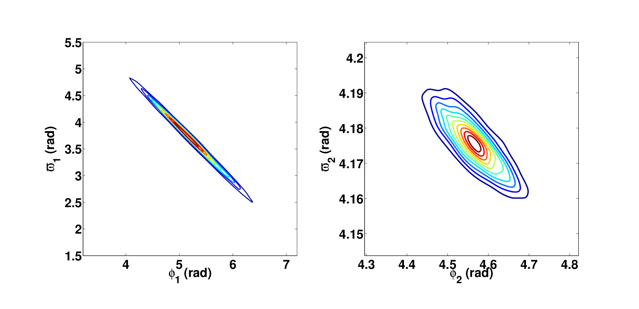
Common MCMC samplers require certain customization to sample ill-shaped densities efficiently [6, 13]. For the density such as the left side of Figure 7, single variable Gibbs sampler updates and isotropic Metropolis samplers require a small step size to achieve a reasonable acceptance probability. But an affine transformation can turn the highly elliptical density on the left to something more spherical, as on the right. The affine invariant MCMC sampler does not view the ill-shaped density on the left more difficult than the well-shaped density on the right[15]. This makes it efficient on many ill-shaped densities, without customization.
Ensemble Sampling
We use an ensemble sampler that updates samples together. An ensemble, , consists of samples, or walkers, . The walkers are samples of the posterior parameter distribution, . The ensemble of walkers is a point in . The target probability density for the ensemble is
| (11) |
That is to say that each walker is an independent sampler of the posterior.
Stretch Move
In the ensemble MCMC sampler, one step of the Markov chain consists of updating all walkers one by one as a whole cycle. Expressed in pseudo code, it is
- for
update
The update step preserves the ensemble sampling density (11), which means that if
has density (11), then has density (11) too. The update of walker uses the current positions of the other walkers in the ensemble, which we call the complementary ensemble:
This is with its most current locations, but with walker omitted.
In this work, we update using the stretch move, defined as follows. The random stretch variable, , has density described below. First, choose another walker , with all walkers in being equally likely. Then propose a move . The proposed new position of lies on the line containing and , but the distance between them is stretched by . Accept with Metropolis probability
| (12) |
where is the dimension of the parameter space. If is accepted, then . Otherwise .
The density of the stretch factor, , must satisfy the symmetry condition
| (13) |
As long as (13) is satisfied, the move satisfies detailed balance for the density (11), see [15]. A simple distribution that satisfies this condition is
| (14) |
The two parameters in the stretch move ensemble sampler are the ensemble size, , and the stretch factor parameter, . The normalization constant is . The method requires in order to sample the entire parameter space. In the runs reported here, we took and . The results are insensitive to ensemble size. The parameters are not tuned for individual star datasets.
IV Local Optima
Local optima of the negative log likelihood function (8) are a problem for many parameter estimation and sampling problems. Local optima correspond to parameter fits that are better than other nearby fits but worse than fits in different parts of parameter space. Figure 1 gives an example for one specific star dataset. While any valid MCMC sampler would eventually find samples near the global optimum, doing so may require an impractically long run. With the initialization just described, after cooling (see below), walkers from the ensemble find themselves in various local probability wells. The computational challenge is twofold. We seek to explore parameter space well enough that at least some of the walkers find the well of the global optimum. We also seek to cluster walkers in the various wells so that we can remove walkers from all but the most important one, or ones.
It is clearly undesirable to manually initialize the MCMC code star-by-star to avoid local optima. To be most useful, a code should find samples near the global optimum by itself. There seems to be no practical way to guarantee this, but our combination of ensemble sampling with simulated annealing and clustering does it more reliably than our earlier codes. Also, the faster equilibration time of the ensemble sampler allows it to move more easily from local well to local well. For HIP36616, we believe our algorithm has identified the global optimum. However, in other datasets, our algorithm failed to find fits as good as those other groups found by hand using the periodogram. Further progress on this issue would be very important in creating automatic data analysis routines that do not require individual human attention for each star. For instance, right now, we only use the periodogram to roughly guess the period (see below), but we could make further use of the periodogram in our code to improve automatization.
Simulated Annealing
Simulated annealing [21] is a Monte Carlo method for finding global optima in problems that have many local optima. It uses a modified posterior distribution with an artificial “inverse temperature” parameter, :
| (15) |
where is the negative log likelihood function (8). Small allows the sampler to explore parameter space freely without getting stuck in local wells. The desired posterior (7) corresponds to . The autocovariance function, described below, decays faster at small . Cooling (increasing ) slowly allows the walkers to find promising local optima. A cooling schedule is an algorithm that increases during the sampling process.
We use simulated annealing in the first phase of our sampler. We initialize the ensemble as a small ball centered at a random position in parameter space except for the dimensions related to the period, for which we use the periodogram [1, 3] to check for peaks between the shortest observation interval and the total observation time to make a guess. As the dataset can reveal periods outside this range, this is not completely reliable. In a one-planet fit, we use the period with the highest peak as the initial period guess unless the data shows a linear trend which indicates a long-period companion. In such cases we use as the period guess. In two-planet fit, is the initial guess for the 1st planet and for the 2nd planet, we use the period of the 2nd highest peak to initialize a portion of walkers and the period of the 3rd highest peak for another portion of walkers and so on. If the data shows a linear trend, we would use as the guess for the 2nd planet. The number is chosen empirically and any reasonably large number should do. Ideally, we want our initialization to be as random as possible to demonstrate the value of the algorithm, but not as random so that the algorithm is unnecessarily sabotaged by the randomness. We initialize by , where is the size of dataset so that only one data matters on average in the beginning. The runs here used the following cooling schedule: is increased in steps and the amount is determined by where is the index of the steps. is kept constant within every one th of the total steps. In general, we used . At the end of the cooling phase the sampler has been using for a while, so the walkers in the ensemble are well equilibrated in their local optima. A typical example is the left frame of Figure 2, with several local optima clearly visible.
Clustering
Figure 1 shows the results for a particular dataset after annealing, for which about of the walkers in the ensemble are in a well that corresponds to an excellent fit. About of the remaining walkers are in another local well that corresponds to a worse fit (see inserts). The negative log likelihood for this worse fit is an order of magnitude larger. The clustering phase of our algorithm seeks to identify clusters of walkers corresponding to the local wells, so that all but the important ones can be removed. The right frame of Figure 1 shows the result in this case. Only walkers from the global optimum remain.
While there are many sophisticated clustering methods, we found that for our problems, a simple one dimensional clustering method is more effective and reliable than the others we tried, such as clustering in parameter space. Note that there could also be multiple local optima due to aliasing, they could have very similar likelihoods. In such cases, we would need more sophisticated clustering methods. After the annealing is finished, but before clustering, we collect the average negative log likelihood function for each walker. (One can also use posterior function, since the normalization constant doesn’t matter when one is taking the difference of posterior.)
This results in the numbers
| (16) |
The idea is that is characteristic of the well walker is in, so that walkers in the same well will have similar . Given , the clustering first ranks all the walkers based on so that is in the order of decreasing , or increasing . There are big jumps in in this sequence (see Figure 1), which are fairly easy to identify and thus to separate the jumps. We calculated the difference in for every adjacent pair of starting from and find the 1st pair whose difference is certain amount of times bigger than the average difference before. So if
| (17) |
all the with are thrown away and only the ones with are kept.
A more rigorous approach to the multiple well/multiple fit problem would be to estimate the evidence integral corresponding to a well before deleting it. It could happen that a small but deep well has less posterior probability than a broad but shallow well. We do not find that this occurs in practice in the fits discussed in this paper. For example, our prior prevents very short-period orbits that might give excellent but spurious fits to the data. The inserts of Figure 1 suggest that the local wells should be removed in our problem. In future work we hope to address this issue more carefully by estimating the evidence integrals. Even then, clustering as we do it here will be the first step.
V Data and results
We tested our code on data from the Lick K-Giant Search [8, 24, 16, 17, 26]. In this paper, we present the results for two stars: HIP36616 and HIP88048. HIP36616 is interesting because the data shows a companion with a small period and small mass and another companion with very large period and very large mass. The information on the large period is incomplete which causes the Metropolis-Hastings algorithm difficulty in finding a good fit. HIP88048 has near complete information on both periods so it is an easier case for Metropolis Hastings and is used as a comparison. Other groups ran these two stars with common Metropolis-Hastings routines. They confirmed that they could easily find a good fit for HIP88048. But for HIP36616, a good fit was found only after new data were obtained. Our code successfully found a fit for HIP36616 before the new data came in.
HIP36616 is interesting and challenging both from a physical and a sampling point of view. The RV data together with a good fit are shown in Figure 3. The data are well explained by a small close companion in a roughly circular orbit and a larger and more distant companion in a highly elliptical orbit. The mass ratio in the posterior distribution (assuming coplanar orbits) is
The parameters with their confidence intervals are listed in Table 2. Histograms of the individual parameters are shown in Figure 4.
The second example fit with the new sampler, HIP88048, is shown in Figure 5. The parameters with their confidence intervals are listed in Table 3. We also run our code on only the first half of the data of HIP88048. We get similar results as with all the data, but with a larger variance, especially for the parameters of the planet with larger period.
VI Comparison with Metropolis-Hastings
All non-trivial MCMC samplers produce autocorrelated samples. An important measure of the effectiveness of the sampler is its covariance of the equilibrium time lag . The longer it takes the covariance to decay to , the longer it takes the sampler to generate independent samples, because non-zero covariance indicates correlation between samples. To be more precise, suppose is some function of the parameters, such as or some nonlinear function of the components. The equilibrium autocovariance function is
The limit is only to ensure that the Monte Carlo has reached steady state. The dimensionless version of this is the autocorrelation function
| (18) |
We used the standard estimators
and
Figure 6 displays the functions , which correspond to taking to be the j-th parameter . Note can be quite different for different components of for the same dataset.
The important measure of correlation for Monte Carlo is the integrated autocorrelation time (summed, actually)
This is the number of Monte Carlo steps needed to produce an effectively independent sample of the posterior, see [15] and references there.
Metropolis Sampler Proposal and Tuning.
For comparison purposes we coded a traditional MCMC sampler that updates the components one at a time using a trial that is uniform in an interval . The ranges were tuned individually for each component to give acceptance probability , which is commonly thought to be roughly optimal. The tuning parameters are different for each , and for a given they are different for each dataset. One can also use Gaussian distribution for trial move which should give similar result.
It is noteworthy that for the Metropolis sampler to work best, one should tune all the free parameters which are on the order of the dimension squared. But how the free parameters are tuned highly depends on where the walker is in the parameter space. That is to say, the free parameters best tuned for a place far from the best-fit optimum in the parameter space could be quite different from those best tuned for a place close to the best-fit optimum. Even if the best-tuned free parameters are similar everywhere in the parameter space, the tuning workload still increases as fast as the parameter space dimension squared.
Comparison.
For the ensemble sampler, we used the ensemble mean
| (19) |
in place of a single value on the right side of (18) in the definition of , in other word, replacing in (18) with defined in (19) (Note the possible confusion of notation: is component of the parameter vector , while is the th parameter vector in an ensemble of such parameter vectors.) It may seem unfair to compare one step of a single vector method to a single step of the ensemble method, given that an ensemble step requires updating walkers rather than one. However, because the walkers in the ensemble are independent (see ( 11)), doing ensemble updates produces effectively independent samples. 11 1 This does not apply to burn in, so that ensemble may suffer more work from burn in phase. Therefore, the ensemble sampler will be exactly as effective as the traditional one if it has the same autocorrelation function [15] .
Two other factors should be mentioned. One is that the traditional sampler requires one likelihood evaluation per component per update, while the ensemble sampler requires one likelihood evaluation per vector update. That is, the traditional sampler uses a factor of (the number of parameters) more likelihood evaluations per vector update. This is a serious consideration in the present application, where likelihood evaluations are the most expensive part of the algorithm. To be sure, in many applications (though not ours) it is not so expensive to update the likelihood function after changing a single parameter. The other is that the ensemble method is more automatic in that it does not require component specific or dataset specific tuning. All the runs reported here used parameters and .
Figure 6 shows the results for the two datasets, each of which is a star with two companions. In both cases, the traditional sampler relaxes the components of the easier companion more quickly, while the ensemble sampler (which updates all parameters together) relaxes all parameters at roughly the same rate. In both cases, the ensemble is much more effective in relaxing the parameters of the difficult companion. In the harder case, HIP36616, the relaxation for the ensemble sampler is at least an order of magnitude faster than the relaxation for the traditional sampler.
VII Discussion
This paper reports progress toward the goal of making posterior sampling fast, reliable, and automatic for exoplanet radial velocity fitting. The sampler presented here performed well and automatically for all the individual star datasets we tried (about a hundred data points). Very high aspect ratio wells and spurious local wells all were handled without individual tuning using a single shell script. Future projects, such as hierarchical modeling of the exoplanet distribution [19], can become impractical with traditional samplers if they are slow. Statistical information about exoplanets, such as the eccentricity distribution [28, 19, 30], the mass distribution [20], the mass-semimajor axis distribution [27], the brown dwarf desert [14, 22], and inclinations [18], depend on rapid and reliable processing of star datasets. It is a limitation of this work that we have used uninformative priors, since we already have plenty of knowledge about exoplanets; we should infer from the collection of all exoplanets priors that improve our fitting for any individual new system. Hierarchical approaches make it possible to infer informative priors without making strong new assumptions. Hierarchical model comparison and selection is a future project, as are projects in which we tune our optimization strategy to operate rapidly and robustly on large numbers of exoplanet systems (a pre-requisite for efficient hierarchical modeling.
We believe that Figure 7 at least partly explains the faster decay of correlations in the ensemble sampler. For the probability distribution in the left frame, traditional single variable updates must have small proposal steps or suffer high rejection rates. For example, if is fixed, then cannot move much and stay within the range of likely parameters. Samplers based on isotropic multivariate proposals must also take small proposal steps. But the ensemble sampler moves walkers along lines between themselves and other walkers, which naturally adapts the proposal steps to the geometry of the distribution.
In our comparison with the Metropolis-Hastings sampler, we didn’t tune the M-H sampler to its full extent. If we did, it is reasonable to think that the performance of the Metropolis-Hastings sampler—locally where it is tuned—would be the same as our ensemble sampler. But tuning free parameters (whose number is on the order of the number of dimensions squared) is already difficult, let alone the fact that best-tuned free parameters could change dramatically as the walker travels in the parameter space. Our ensemble sampler emulates a best-tuned Metropolis-Hastings sampler, best-tuned wherever the walker goes.
One of the problems we have encountered is that our ensemble sampler is greatly affected by the existence multiple local optima. If the walkers occupy different local optima, the acceptance ratio can be greatly lowered because the proposed moves are based on walkers from other optima. In this case, the proposal may be outside any well and therefore unlikely to be accepted. The clustering we propose and use here is a great help in this regard, and effectively overcomes this problem. And our runs never encountered more than one statistically significant local optima.
The ensemble sampler may also be better suited for high performance computing. Each walker in the ensemble evolves in parallel. Our current implementations do not exploit this parallelism; more sophisticated software designed for high performance hardware would be welcome.
We believe that more sophisticated methods from machine learning could have a large impact on these sampling problems. One obvious application would be more sophisticated clustering methods. Another would be to make more use of the information in the ensemble to build a model of the posterior. For example [15] speculate that one could use half of the ensemble to build a nonlinear model of the posterior that would allow the other half of the ensemble to be re-sampled more effectively
All of the software used for this project is available upon request. Included in this is a general purpose of the ensemble sampler that can be used for other sampling problems.
References
- [1] Bretthorst, G., L., 1988, Bayesian Spectrum Analysis and Parameter Estimation (New York: Springer-Verlag)
- [2] Brooks, S., Gelman, A., Jones, G. L., Meng, X. -L., 2011, Handbook of Markov Chain Monte Carlo (Chapman & Hall)
- [3] Cumming, A., 2004, MNRAS, 354, 1165
- [4] Driscoll, P., 2006, A Comparison of Least-Squares and Bayesian Fitting Techniques to Radial Velocity Data Sets, Master’s Thesis, San Francisco State University
- [5] Ford, E. B., 2005, AJ, 129, 1706
- [6] Ford, E. B., 2006, ApJ, 642, 505
- [7] Ford, E. B., Gregory, P. C., 2006, http://arxiv.org/abs/astro-ph/0608328v1
- [8] Frink, S., et al., 2002, ApJ, 576, 478
- [9] Gilks, R. W., Roberts, G. O., 1994, J. Multivariate Analysis. 49, 287
- [10] Gilks, R. W., Richardson, S. & Spiegelhalter, D. J., 1996, Markov Chain Monte Carlo in Practice (Chapman & Hall)
- [11] Gregory, P. C., Loredo, T. J., 1992, ApJ, 398, 146
- [12] Gregory, P. C., 2005, ApJ, 631, 1198
- [13] Gregory, P. C., 2011, MNRAS, 410, 94
- [14] Grether, D., Lineweaver, C. H., 2006, ApJ, 640, 1051
- [15] Goodman, J., Weare, J., 2010, Comm. App. Math. and Comp. Sci., 5, 65
- [16] Hekker, S., et al., 2006, A&A, 454, 943
- [17] Hekker, S., et al., 2008, A&A, 480, 215
- [18] Ho, S., Turner, E., L., 2010, http://arxiv.org/abs/1003.4738v2
- [19] Hogg, D. W., Myers, A. D. & Bovy, J., 2010, http://arxiv.org/abs/1008.4146v2
- [20] Howard, A. W., et al., 2010, Science, 330, 653
- [21] Kirkpatrick, S., Gelatt, C. D., Vecchi, M. P., 1983, Science, 220, 671
- [22] Leconte, J., et al., 2010, ApJ, 716, 1551
- [23] Loredo, T. J., 1999, ASP Conference Series, 172, 297
- [24] Mitchell, D. S., et al., 2003, BAAS, 35, 1234
- [25] Ohta, Y., Taruya, A. & Suto, Y., 2005, ApJ, 622, 1118
- [26] Quirrenbach, A., Reffert, S. & Bergmann, C., 2011, AIP Conference Proceedings, 1331, 102
- [27] Schlaufman, K. C., Lin, D. N. C. & Ida, S., 2009, ApJ, 691, 1322
- [28] Shen, Y., Turner, E. L., 2008, ApJ, 685, 553
- [29] Wandelt, B. D., Larson, D. L. & Lakshminarayanan, A., 2004, Physics Review D, 70, 083511
- [30] Zakamska, N. L., Pan, M. & Ford, E. B., 2010, http://arxiv.org/abs/1008.4152v1
| Parameter | Variable | Prior | Mathematical Form |
|---|---|---|---|
| Amplitude | Jefferys | ||
| Period | Jefferys | ||
| Orbital Phase | Uniform | ||
| Eccentricity | Uniform | ||
| Longitude of Periastron | Uniform | ||
| Jitter | Jefferys | ||
| Reference Velocity | Uniform |
| parameter | median | CI | CI |
|---|---|---|---|
| 133.9640 | |||
| 5.26268 | |||
| 0.0557283 | |||
| 3.57290 | |||
| 4015.00 | |||
| 4.57002 | |||
| 0.734762 | |||
| 4.17465 | |||
| 18.4083 | |||
| -249.559 |
| parameter | median | CI | CI |
|---|---|---|---|
| 288.108 | |||
| 4.12983 | |||
| 0.129846 | |||
| 1.73223 | |||
| 175.842 | |||
| 3.85943 | |||
| 0.194608 | |||
| 1.76762 | |||
| 7.7662 | |||
| -39.1676 |