跳到论文正文
W Papers独立论文阅读器 arXiv:1104.2589 论文正文 计算阅读时间 · 0%
引用这篇论文根据当前论文元数据生成,正式投稿前建议核对。


License: arXiv.org perpetual non-exclusive license
arXiv:1104.2589v3 [hep-th] 24 May 2011

On 3d extensions of AGT relation

D.Galakhov ††thanks: ITEP, Moscow, Russia and MIPT, Dolgoprudny, Russia; galakhov@itep.ru    A.Mironov Note: Lebedev Physics Institute and ITEP, Moscow, Russia; mironov@itep.ru; mironov@lpi.ru    A.Morozov ††thanks: ITEP, Moscow, Russia; morozov@itep.ru    A.Smirnov ††thanks: ITEP Moscow, Russia and MIPT, Dolgoprudny, Russia; asmirnov@itep.ru

FIAN/TD-04/11

ITEP/TH-10/11

ABSTRACT

An extension of the AGT relation from two to three dimensions begins from connecting the theory on domain wall between some two S-dual SYM models with the 3d Chern-Simons theory. The simplest kind of such a relation would presumably connect traces of the modular kernels in 2d conformal theory with knot invariants. Indeed, the both quantities are very similar, especially if represented as integrals of the products of quantum dilogarithm functions. However, there are also various differences, especially in the ”conservation laws” for integration variables, which hold for the monodromy traces, but not for the knot invariants. We also discuss another possibility: interpretation of knot invariants as solutions to the Baxter equations for the relativistic Toda system. This implies another AGT like relation: between 3d Chern-Simons theory and the Nekrasov-Shatashvili limit of the 5d SYM.

1 Introduction

In [1] (see also [2]-[12]) a long expected relation was suggested, which can be considered as one of possible 3+3 counterparts of the celebrated 2+4 AGT relation [13] between conformal blocks and Nekrasov functions. This new relation is supposed to identify the modular transformation kernels M⁡(a,a′)M(a,a^{\prime}) of conformal blocks and matrix elements in 3​d3d Chern-Simons theory. In its simplest version, relation is between the trace of the modular kernel, considered as a function of external dimensions, and Hikami integrals [14], representing the Chern-Simons partition functions on S3/KS^{3}/K (a 3​d3d sphere with a knot KK removed) considered as functions of monodromies around KK. A modest task of this letter is to discuss possible formulations of such a relation in an explicit form, leaving aside all the general context and reasoning, discussed in great detail in the profound text [1]. We point out some problems with exact identification of the modular trace and the knot invariants. We also attract attention to another similarity: between the knot invariants and 5​d5d Seiberg-Witten theory, which implies still another kind of AGT relation, involving the 3​d3d Chern-Simons theory.

2 Modular kernel

The conformal block BΓ​(a​|m|​q)B_{\Gamma}(a|m|q) for a given graph Γ\Gamma depends on three kinds of variables: aa and mm are parameters (α\alpha-parameters) on internal lines and external legs respectively (the corresponding conformal dimensions are quadratic in these parameters), and qq parameterizes the graph itself. The modular transformation does not change the graph Γ\Gamma, while changing q→q′q\rightarrow q^{\prime} and permuting the entries within the set α\alpha of external-legs parameters and is realized as an integral transform in aa variables:

BΓ​(a​|α|​q)=∫M⁡(a,a′)​BΓ​(a′​|α′|​q′)​𝑑μ​(a′)\displaystyle B_{\Gamma}(a|\alpha|q)=\int M(a,a^{\prime})B_{\Gamma}(a^{\prime}|\alpha^{\prime}|q^{\prime})d\mu(a^{\prime}) (1)

The function M⁡(a,a′)M(a,a^{\prime}) depends on Γ\Gamma and α\alpha, but not on qq, and is called the modular kernel, associated with the particular modular transformation q→q′q\rightarrow q^{\prime}. In spirit, it is a Fourier kernel:

M⁡(a,a′)∼exp⁡(4​π​i​a​a′ϵ1​ϵ2+…)\displaystyle M(a,a^{\prime})\sim\exp\left(\frac{4\pi iaa^{\prime}}{\epsilon_{1}\epsilon_{2}}+\ldots\right) (2)

where the corrections are less singular at small ϵ1\epsilon_{1} and ϵ2\epsilon_{2}.

0 , Δ α Δ a
Figure 1: Toric conformal block diagram, Δa=ϵ2/4+a2ϵ1​ϵ2\Delta_{a}=\frac{\epsilon^{2}/4+a^{2}}{\epsilon_{1}\epsilon_{2}} , Δα=ϵ2/4+α2ϵ1​ϵ2\Delta_{\alpha}=\frac{\epsilon^{2}/4+\alpha^{2}}{\epsilon_{1}\epsilon_{2}} .

The simplest example is provided by the modular transformation of the toric 1-point function, Fig.1 which on the gauge theory side describes the theory with adjoint matter with mass m=−i​α+ϵ2=−2​i​α~m=-i\alpha+{\epsilon\over 2}=-2i\tilde{\alpha}:

ℬ⁡(a​|α|−1/τ)=∫ℳ⁡(a,a′|α)​ℬ​(a′​|α|​τ)​𝑑μ​(a′)\displaystyle{\cal B}\big(a\big|\alpha\big|-1/\tau\big)=\int{\cal M}(a,a^{\prime}|\alpha){\cal B}\big(a^{\prime}\big|\alpha\big|\tau\big)d\mu(a^{\prime}) (3)

Here [15]

ℬ(a|α|τ)=q−(ν+1)/24η(q)νe2​π​i​τ​a2ϵ1​ϵ2(1+2q(ϵ1−m)​(ϵ2−m)ϵ1​ϵ2(ϵ2−4​a2+m⁡(m−ϵ))(ϵ2−4​a2)+O(q2))\displaystyle{\cal B}(a|\alpha|\tau)=q^{-(\nu+1)/24}\eta(q)^{\nu}e^{\frac{2\pi i\tau a^{2}}{\epsilon_{1}\epsilon_{2}}}\left(1+2q\frac{(\epsilon_{1}-m)(\epsilon_{2}-m)}{\epsilon_{1}\epsilon_{2}}\frac{\big(\epsilon^{2}-4a^{2}+m(m-\epsilon)\big)}{(\epsilon^{2}-4a^{2})}+O(q^{2})\right) (4)

with ν=1−2​m​(ϵ−m)ϵ1​ϵ2\nu=1-\frac{2m(\epsilon-m)}{\epsilon_{1}\epsilon_{2}}, ϵ=ϵ1+ϵ2\epsilon=\epsilon_{1}+\epsilon_{2} and η⁡(q)=q124​∏k=1∞(1−qk)\eta(q)=q^{\frac{1}{24}}\prod\limits_{k=1}^{\infty}(1-q^{k}), q=e2​π​i​τq=e^{2\pi i\tau}. According to [16] the modular kernel is given by

ℳ⁡(a,a′|α)=23/2s⁡(α)​∫s⁡(a+r+α~)​s​(a−r+α~)s⁡(a+r−α~)​s​(a−r−α~)​e4​π​i​r​a′ϵ1​ϵ2​𝑑r\displaystyle{\cal M}(a,a^{\prime}|\alpha)=\frac{2^{3/2}}{s(\alpha)}\int\frac{s(a+r+\tilde{\alpha})s(a-r+\tilde{\alpha})}{s(a+r-\tilde{\alpha})s(a-r-\tilde{\alpha})}\ e^{\frac{4\pi ira^{\prime}}{\epsilon_{1}\epsilon_{2}}}dr (5)

where the measure is

d​μ​(a′)=4​sinh⁡(2​π​ϵ1​a′)​sinh⁡(2​π​ϵ2​a′)​d​a′\displaystyle d\mu(a^{\prime})=4\sinh(2\pi\epsilon_{1}a^{\prime})\sinh(2\pi\epsilon_{2}a^{\prime})da^{\prime} (6)

The function s⁡(z)s(z) is the ”quantum dilogarithm” [17, 18], the ratio of two digamma-functions [17],

s⁡(z|ϵ1,ϵ2)∼∏m,n≥0(m+12)​ϵ1+(n+12)​ϵ2−i​z(m+12)​ϵ1+(n+12)​ϵ2+i​z\displaystyle s(z|\epsilon_{1},\epsilon_{2})\sim\prod_{m,n\geq 0}\frac{\left(m+\frac{1}{2}\right)\epsilon_{1}+\left(n+\frac{1}{2}\right)\epsilon_{2}-iz}{\left(m+\frac{1}{2}\right)\epsilon_{1}+\left(n+\frac{1}{2}\right)\epsilon_{2}+iz} (7)

Note that ℳ⁡(a,a′|α){\cal M}(a,a^{\prime}|\alpha) depends on the external momentum α~\tilde{\alpha}, the internal dimension Δ⁡(α)\Delta(\alpha) and the central charge c=1+6​ϵ2ϵ1​ϵ2c=1+6\frac{\epsilon^{2}}{\epsilon_{1}\epsilon_{2}}, but not on the modular parameter τ\tau.

When α→0\alpha\rightarrow 0, the conformal block becomes pure classical: ℬ⁡(a​|α|​τ)→1η⁡(q)​e2​i​π​τ​a2/ϵ1​ϵ2{\cal B}(a|\alpha|\tau)\rightarrow\frac{1}{\eta(q)}\ e^{2i\pi\tau a^{2}/\epsilon_{1}\epsilon_{2}} (the last factor in the brackets in (4) turns into q1/12​η−2​(q)q^{1/12}\eta^{-2}(q) when m=0m=0), and the modular transformation turns into the ordinary Fourier transform:

ℳ⁡(a,a′|0)​μ′​(a)⟹α~=i​ϵ/22​cos⁡(4​π​i​a​a′ϵ1​ϵ2)\displaystyle{\cal M}(a,a^{\prime}|0)\mu^{\prime}(a)\ \ \ \stackrel{{\scriptstyle\tilde{\alpha}=i\epsilon/2}}{{\Longrightarrow}}\ \ \ \sqrt{2}\cos\left(4\pi i\frac{aa^{\prime}}{\epsilon_{1}\epsilon_{2}}\right) (8)

so that indeed

e−2πiτ−1a2/(ϵ1ϵ2)η⁡(−τ−1)=∫d​a′ϵ1​ϵ2​e4​π​i​a​a′/(ϵ1​ϵ2)​e2​π​i​τ​a′2/(ϵ1​ϵ2)η⁡(τ)\displaystyle\frac{e^{-2\pi i\tau^{-1}a^{2}/(\epsilon_{1}\epsilon_{2})}}{\eta(-\tau^{-1})}=\int\frac{da^{\prime}}{\sqrt{\epsilon_{1}\epsilon_{2}}}e^{4\pi iaa^{\prime}/(\epsilon_{1}\epsilon_{2})}\frac{e^{2\pi i\tau a^{\prime 2}/(\epsilon_{1}\epsilon_{2})}}{\eta(\tau)} (9)

It is a somewhat non-trivial exercise to deduce (8) from eq.(5), see Appendix A for the simplified case ϵ1=−ϵ2=gs\epsilon_{1}=-\epsilon_{2}=g_{s}.

Notice that the monodromy kernel satisfies the unitarity relation

∫d​μ​(a)​M​(a,b)​M∗​(a,b′)=d​μ​(b′)d​b′​δ​(b−b′)\displaystyle\int d\mu(a)M(a,b)M^{*}(a,b^{\prime})=\frac{d\mu(b^{\prime})}{db^{\prime}}\delta(b-b^{\prime}) (10)

Therefore, it is natural to define the trace as Tr∼∫d​μ​(a)d​μ​(a′)​d​a′​δ​(a−a′){\rm Tr}\sim\int\frac{d\mu(a)}{d\mu(a^{\prime})}da^{\prime}\delta(a-a^{\prime}). Thus defined trace of the monodromy kernel (5) contains two integrals, but they actually split:

∫ℳ⁡(a,a|α)​𝑑a=23/2s⁡(α)​∫∫s⁡(a+r+α~)​s​(a−r+α~)s⁡(a+r−α~)​s​(a−r−α~)​e4​π​i​r​a​𝑑r​𝑑a=23/2s⁡(α)​T+​(α~)​T−​(α~)\displaystyle\int{\cal M}(a,a|\alpha)da=\frac{2^{3/2}}{s(\alpha)}\int\int\frac{s(a+r+\tilde{\alpha})s(a-r+\tilde{\alpha})}{s(a+r-\tilde{\alpha})s(a-r-\tilde{\alpha})}\ e^{4\pi ira}drda=\frac{2^{3/2}}{s(\alpha)}T_{+}(\tilde{\alpha})T_{-}(\tilde{\alpha}) (11)

where

T±​(α~)=∫s⁡(z+α~)s⁡(z−α~)​e±i​π​z2​𝑑z\displaystyle T_{\pm}(\tilde{\alpha})=\int\frac{s(z+\tilde{\alpha})}{s(z-\tilde{\alpha})}\ e^{\pm i\pi z^{2}}dz (12)

In fact, the quantities like T±​(α~)T_{\pm}(\tilde{\alpha}) are well known from Chern-Simons theory, and this opens a way towards 3​d3d extensions of the AGT conjecture.

3 Exempts from the knot theory

The polynomial knot invariants can be defined as averages of the Wilson loop along the knot in the topological Chern-Simons (CS) theory [19]:

<K>R=⟨TrRPexp∮KA⟩C​S\displaystyle<K>_{R}=\left<{\rm Tr}\,\!_{R}P\!\exp\oint_{K}A\right>_{CS} (13)

This invariant depends on the knot KK, Lie algebra GG, its representation RR, the CS coupling constant ℏ=log⁡q=2​π​ik\hbar=\log q=\frac{2\pi i}{k} (sometimes kk is shifted to k+CAk+C_{A}, as in the WZNW model [20]), and, additionally, on the monodromy uu, which describes deviation from the periodicity of the field AA while circling around the knot. One may think of uu as of the eigenvalue of P​S​L​(2)PSL(2) monodromy matrix around the knot KK. On the other hand, one may think that uu takes value in the Cartan subalgebra of the gauge group S​U​(2)SU(2), and, in this way, describes the representation RR living on the knot KK.

The averages <K>R<K>_{R} are clever generalizations of the ordinary characters and, as all exact correlators, possess hidden integrability properties [21, 25]. As a manifestation of this hidden structure, the averages <K>R<K>_{R} satisfy KK-dependent difference equations in the RR(!) variable [26], which allows one to consider them as belonging to the family of generalized qq-hypergeometric series. A q→1q\to 1 limit of these equations defines the spectral curve Σ⁡(K)\Sigma(K) and the saddle point of the corresponding integral representation defines the associated Seiberg-Witten (SW) differential. After that, the full ℏ\hbar-dependence can be reconstructed with the help of the AMM/EO topological recursion [27] from this SW data [9].

A nice property of invariants (13) is that at u=0u=0 they are finite polynomials in q=exp⁡(2​π​ik)q=\exp(\frac{2\pi i}{k}). In the literature, these polynomials normalized by the quantum dimension have different conventional names corresponding to the choice of the group and representation. Here, for convenience we represent a table explaining the correspondence:

Group\RepresentationFundamental representationGeneral representation with weightλN=0Convey-Alexander polynomial–S​U​(2)Jones polynomialColored Jones polynomialS​U​(N)HOMFLY polynomialColored HOMFLY polynomialS​O​(N)Kauffmann polynomialColored Kauffman polynomial{S​U​(N)}tsuperpolynomialColored superpolynomial\begin{array}[]{|c|c|c|}\hline\cr&&\\ \textrm{Group}\backslash\textrm{Representation}&\textrm{Fundamental representation}&\textrm{General representation with weight}\ \ \lambda\\ &&\\ \hline\cr&&\\ N=0&\textrm{Convey-Alexander polynomial}&\textrm{--}\\ &&\\ \hline\cr&&\\ SU(2)&\textrm{Jones polynomial}&\textrm{Colored Jones polynomial}\\ &&\\ \hline\cr&&\\ SU(N)&\textrm{HOMFLY polynomial}&\textrm{Colored HOMFLY polynomial}\\ &&\\ \hline\cr&&\\ SO(N)&\textrm{Kauffmann polynomial}&\textrm{Colored Kauffman polynomial}\\ &&\\ \hline\cr&&\\ \left\{SU(N)\right\}_{t}&\textrm{superpolynomial}&\textrm{Colored superpolynomial}\\ &&\\ \hline\cr\end{array}

The last line of this table describes an extension from (quantum) groups to MacDonald characters which leads to a one-parametric deformation (tt-deformation) of (13), to superpolynomials [22, 23] involving the Khovanov homology [24]. Further extension from MacDonald to the Askey-Wilson-Kerov level remains untouched so far.

Six kinds of representations are currently known for the Wilson averages in Chern-Simons theory, we briefly describe them in the following subsections and provide some explicit examples in Appendix B.

3.1 Representation through quantum RR-matrix [28]

This representation appears when calculations in CS theory are done in the temporal gauge A0=0A_{0}=0 [29]. Then the propagator is ultralocal, and only the crossings (cc) and extremal (ee) points in projection of KK on the x​yxy plane contribute, and the answer can be schematically written as

<K>R=TrR∏e,c→𝒰eℛc\displaystyle<K>_{R}={\rm Tr}\,\!_{R}\overrightarrow{\prod_{e,c}}\ {\cal U}_{e}{\cal R}_{c} (14)

where the ordered product is taken along the line KK, ℛ{\cal{R}} is the quantum RR-matrix in representation RR, and 𝒰=qρ{\cal{U}}=q^{\rho} is the ”enhancement” of the ℛ{\cal R}-matrix in the same representation. For the braid representation of the knot, this formula reduces to the well-known formula for the quantum group invariants of knot:

<K>R=q−w⁡(bK)​Ω2​(R)qtrR(bK)\displaystyle<K>_{R}=q^{-w(b_{K})\,\Omega_{2}(R)}\,{\rm qtr}\,_{R}(b_{K}) (15)

Here bK∈Bnb_{K}\in B_{n} is the element of the braid group, representing the knot KK, i.e. its closure gives KK, Ω2​(R)=trR​(Ta​Ta)/dimR\Omega_{2}(R)={\rm tr}\,_{R}(T^{a}T^{a})/\dim R is the value of quadratic Casimir function in the representation RR and qtrR{\rm qtr}\,_{R} is the quantum trace over the representation RR, qtrR​bK=trR​bK​qρ⊗n{\rm qtr}\,_{R}b_{K}={\rm tr}\,_{R}b^{K}q^{\rho^{\otimes n}}. The function w⁡(bk)w(b_{k}) is the so called writhe number of the braid bKb_{K}, it is equal to the total sum of orientations of the crossings:

bK=∏{k}gknk⟹w⁡(bK)=∑{k}nkb_{K}=\prod\limits_{\{k\}}g_{k}^{n_{k}}\ \ \ \Longrightarrow\ \ \ w(b_{K})=\sum\limits_{\{k\}}\,n_{k}

Calculation of (15) for some particular knot is just a matter of multiplication and taking a trace of relatively big matrices. The braid representations of several first knots and the writhe numbers of the corresponding closures are summarized in the following table:

KnotBraid representationWrithe31b=g13∈B2w⁡(b^)=341b=g2​2​g1−1​g2​g1−1∈B3w⁡(b^)=151b=g15∈B2w⁡(b^)=552b=g23​g1​g2−1​g1∈B3w⁡(b^)=461b=g1​g2−1​g3​g1​g2−1​g3−2∈B4w⁡(b^)=−1\displaystyle\begin{array}[]{|l|l|l|}\hline\cr\textrm{Knot}&\textrm{Braid representation}&\textrm{Writhe}\\ \hline\cr 3_{1}&b=g_{1}^{3}\in B_{2}&w({\hat{b}})=3\\ \hline\cr 4_{1}&b=g_{2}2\,g_{1}^{-1}\,g_{2}\,g_{1}^{-1}\in B_{3}&w({\hat{b}})=1\\ \hline\cr 5_{1}&b=g_{1}^{5}\in B_{2}&w({\hat{b}})=5\\ \hline\cr 5_{2}&b=g_{2}^{3}\,g_{1}\,g_{2}^{-1}\,g_{1}\in B_{3}&w(\hat{b})=4\\ \hline\cr 6_{1}&b=g_{1}\,g_{2}^{-1}\,g_{3}\,g_{1}\,g_{2}^{-1}\,g_{3}^{-2}\in B_{4}&w({\hat{b}})=-1\\ \hline\cr\end{array}

3.2 Representation through classical RR-matrix and quantum associator [30]

A similar representation for <K>R<K>_{R} trough classical instead of quantum RR-matrices appears in the calculation of (13) in the holomorphic gauge Az¯=0A_{\bar{z}}=0. However, instead of the trivial insertions of qρq^{\rho} factors one now needs to insert sophisticated Drinfeld associators [31]. In the holomorphic gauge the theory reduces to the Kontsevich integral of knot [32]. In this case, one can construct the representation of the braid group BnB_{n} in R⊗nR^{\otimes n} though the Drinfeld associators as follows: for the element gk∈Bng_{k}\in B_{n} one has:

gk→ΨkRkΨk−1,Ri=1⊗1⊗…⊗1⏟1​…​i−1⊗R⊗1⊗…⊗1⏟i+2​…​n,withR=qTa⊗Ta\displaystyle g_{k}\rightarrow\Psi_{k}R_{k}\,\Psi_{k}^{-1},\ \ R_{i}=\underbrace{1\otimes 1\otimes...\otimes 1}_{1...i-1}\,\otimes\,R\otimes\underbrace{1\otimes...\otimes 1}_{i+2...n},\ \ \textrm{with}\ \ R=q^{T^{a}\otimes T^{a}} (23)

Ψk=Φk⊗1⊗(n−k)\Psi_{k}=\Phi_{k}\otimes 1^{\otimes(n-k)}, where Φk\Phi_{k} is the kk-th Drinfeld associator. Then, again, if bK∈Bnb_{K}\in B_{n} is the braid representing some knot KK, for the quantum invariant (13) one obtains

<K>R=qtrR(1)nq−w⁡(bK)​Ω2​(R)qtrR(bK)\displaystyle<K>_{R}={\rm qtr}\,_{R}(1)^{n}\,q^{-w(b_{K})\,\Omega_{2}(R)}\,{\rm qtr}\,_{R}(b_{K}) (24)

Again, the classical RR-matrices R=qTa⊗TaR=q^{T^{a}\otimes T^{a}} stand just at the intersection points of the KK projection on a plane. However, instead of the simple enhancement factors qρq^{\rho}, one now inserts in between the quantum associators [31], acting on kk lines simultaneously. The Drinfeld associators are solutions to the Knizhnik-Zamolodchikov equations [33] in the WZNW conformal theory [20]. In particular, the kk-th associator describes the monodromy of k+2k+2-point function in the WZNW model, and the Kontsevich integral (24) is nothing but the trace of monodromy associated with the braid bKb_{K}. For further details of this representation see [34].

3.3 Representation through Vassiliev invariants and Kontsevich integrals

In CS theory perturbative expansion, the dependencies of the Wilson average <K>R<K>_{R} on the knot KK and on the group structure G,RG,R are nicely separated:

<K>R=dimq(R)∏m=0∞∏n=1dmexp(ℏmαm,n(K)rm,n(R))\displaystyle<K>_{R}\,=\dim_{q}(R)\prod\limits_{m=0}^{\infty}\,\prod_{n=1}^{d_{m}}\,\exp\Big(\hbar^{m}\alpha_{m,n}(K)\,r_{m,n}(R)\Big) (25)

where d​i​mq​(R)dim_{q}(R) is the quantum dimension of representation:

dimq(R)=qN2−q−N2q12−q−12\dim_{q}(R)=\dfrac{q^{{N\over 2}}-q^{-{N\over 2}}}{q^{1\over 2}-q^{-{1\over 2}}}

The quantities αm,n​(K)\alpha_{m,n}(K) are the primary Vassiliev invariants [35], which are rational(!) numbers, naturally represented either as modifications of the Gauss linking integrals in the Lorentz gauge ∂μAμ=0\partial_{\mu}A_{\mu}=0 [36], or as the Kontsevich integrals [32] in the holomorphic gauge Az¯=0A_{\bar{z}}=0, or through the writhe numbers [37] in the temporal gauge A0=0A_{0}=0.

The group factors rm,nr_{m,n} are the eigenvalues of operators from the cut-and-join algebra [38] on the G​L​(∞)GL(\infty) characters χR\chi_{R}, and form a basis of the multiplicative independent Casimir eigenvalues of order mm. In every order mm one has dmd_{m} independent Casimirs, the first several values are:

m123456dm011235\begin{array}[]{|c|c|c|c|c|c|c|}\hline\cr m&1&2&3&4&5&6\\ \hline\cr d_{m}&0&1&1&2&3&5\\ \hline\cr\end{array} (26)

rk​j​(R)r_{kj}(R) can be also understood as eigenvalues of operators from the cut-and-join algebra [38] on the characters χR\chi_{R}, and are certain non-linear combinations of the Casimir eigenvalues. The Casimir functions rm,nr_{m,n} are polynomials of the rank and the weight of the representations, the following table lists the first four Casimirs for S​U​(n)SU(n), S​O​(n)SO(n) in the fundamental representation and for S​U​(2)SU(2) in the spin JJ representation:

r2,1r3,1r4,1r4,2S​U​(n)fund.−n2−14−n⁡(n2−1)8−n2​(n2−1)16−(n2+2)​(n2−1)16S​O​(n)fund.−(n−2)​(n−1)16−(n−2)2​(n−1)64−(n−2)3​(n−1)256(n−1)​(n−2)​(n2−5​n+10)256S​U​(2),J−J⁡(J+1)−J⁡(J+1)−J⁡(J+1)2​J2​(J+1)2\displaystyle\begin{array}[]{|l|l|l|l|l|}\hline\cr&r_{2,1}&r_{3,1}&r_{4,1}&r_{4,2}\\ \hline\cr&&&&\\ SU(n)\ \ \textrm{fund.}&-\frac{n^{2}-1}{4}&-\frac{n(n^{2}-1)}{8}&-\frac{n^{2}(n^{2}-1)}{16}&-\frac{(n^{2}+2)(n^{2}-1)}{16}\\ &&&&\\ SO(n)\ \ \textrm{fund.}&-\frac{(n-2)(n-1)}{16}&-\frac{(n-2)^{2}(n-1)}{64}&-\frac{(n-2)^{3}(n-1)}{256}&\frac{\left(n-1\right)\left(n-2\right)\left({n}^{2}-5\,n+10\right)}{256}\\ &&&&\\ SU(2),\ \ J&-J(J+1)&-J(J+1)&-J(J+1)&2J^{2}(J+1)^{2}\\ &&&&\\ \hline\cr\end{array}

Our choice of the basis of rm,nr_{m,n} is shown in Fig.2 in the form of the chord diagrams: the circle stands for the trace over representation RR, and the trivalent vertices depict the structure constants fa​b​cf^{abc} of the algebra. This notation is clear from the two examples:

r2,1=1dimR​fa​b​c​trR​(Ta​Tb​Tc),r3,1=1dimR​fa​b​e​fe​c,d​trR​(Ta​Tb​Td​Tc)r_{2,1}=\frac{1}{\dim_{R}}f^{abc}{\rm tr}\,_{R}(T^{a}T^{b}T^{c}),\ \ \ \ \ r_{3,1}=\dfrac{1}{\dim_{R}}f^{abe}f^{ec,d}{\rm tr}\,_{R}(T^{a}T^{b}T^{d}T^{c})

In the case of G=S​L​(2)G=SL(2) the relevant representations RR are labeled by the value of spin JJ, and rk​j​(J)r_{kj}(J) are polynomials of JJ of degree kk. The series in the exponential (25) can be re-expanded in new variables ℏ\hbar and N=2​J+1=u/ℏN=2J+1=u/\hbar:

F(K,ℏ,u)=log<K>R−logN=∑k=0∞ℏk∑j=1dkαk​j(K)rk​j(N/ℏ)=∑kℏkFk(K,u)\displaystyle F(K,\hbar,u)=\log<K>_{R}-\log N=\sum_{k=0}^{\infty}\hbar^{k}\sum_{j=1}^{d_{k}}\alpha_{kj}(K)r_{kj}(N/\hbar)=\sum_{k}\hbar^{k}F_{k}(K,u) (36)

These Fk​(K,u)F_{k}(K,u) are infinite combinations of Vassiliev invariants of all orders. The K−JK-J\ separation gets obscure after such a re-expansion, and all the information about the gauge group (rm,nr_{m,n}) and the knot (αm,n\alpha_{m,n}) gets mixed. Instead this expansion is the knot theory counterpart of the genus (1/N1/N) expansion in matrix models, and u=ℏ​Nu=\hbar N plays role of the t’Hooft’s coupling.

Remarkably, for some knots (called hyperbolic) F⁡(K)F(K) behaves as V⁡(K,u)​ℏ−1V(K,u)\hbar^{-1} at small ℏ\hbar [39], this is despite all terms in the series have positive powers of ℏ\hbar! This is typical for genus expansion series: contributions of every particular genus are all convergent series, but the sum over genera diverges: it can be studied with the help of the Pade summation methods, see [40, 41] for a recent description within the matrix model context. The value of the coefficient V⁡(K,u=1)V(K,u=1) at u=1u=1 coincides with the volume of S3/KS^{3}/K in the uniquely defined hyperbolic metric [42], the situation is far more interesting for non-hyperbolic knots (toric or satellite), see the plots in appendix C.

Refer to caption
Figure 2: A basis of independent Casimir function up to degree 66.

3.4 Representation through quantum dilogarithm

In [26] the polynomial invariants (13) for the gauge group S​U​(2)SU(2) with spin JJ were systematically interpreted as generalized qq-hypergeometric functions, such representations were widely used before in particular examples. This means that these Wilson averages can be represented in the form of finite sums:

<K>J=dimq(R)∑k1,k2,…,kn(q,N)k1​…​(q,N)i1(q,N)ki2​…​(q,N)knqp2​(k1,…,kn)\displaystyle<K>_{J}=\dim_{q}(R)\sum\limits_{k_{1},k_{2},...,k_{n}}\dfrac{(q,N)_{k_{1}}...(q,N)_{i_{1}}}{(q,N)_{k_{i_{2}}}...(q,N)_{k_{n}}}\,q^{p_{2}(k_{1},...,k_{n})} (37)

Here N=2​J+1N=2J+1, (q,N)k(q,N)_{k} is the qq-Pochhammer symbol:

(q,N)k=∏i=1k(qN−i2−q−N−i2)\displaystyle(q,N)_{k}=\prod\limits_{i=1}^{k}\Big(q^{\frac{N-i}{2}}-q^{-\frac{N-i}{2}}\Big)\ (38)

and p2​(k1,…,kn)p_{2}(k_{1},...,k_{n}) is a certain quadratic function. The numbers of kik_{i} in the sum (37), the quadratic polynomial p2p_{2}, the arrangement of the Pochhammer symbols are determined by the knot KK and the limits of summation by JJ . The existence of such a representation for knots directly follows from the A​JAJ-conjecture for the colored Jones polynomials [43], which states that <K>j<K>_{j} is a solution of certain hypergeometric difference equation, see also s.3.6 below. At the same time, the Pochhammer symbols can be expressed through the ratio of the quantum dilogarithms:

(q,N)k=(−i)k​s⁡(i​ϵ2​(N−1−k)+i2​(ϵ1+ϵ2)|ϵ1,ϵ2)s⁡(i​ϵ2​(N−1)+i2​(ϵ1+ϵ2)|ϵ1,ϵ2)\displaystyle(q,N)_{k}=(-i)^{k}\,\dfrac{s\left(i\epsilon_{2}(N-1-k)+\frac{i}{2}(\epsilon_{1}+\epsilon_{2})\Big|\epsilon_{1},\epsilon_{2}\right)}{s\left(i\epsilon_{2}(N-1)+\frac{i}{2}(\epsilon_{1}+\epsilon_{2})\Big|\epsilon_{1},\epsilon_{2}\right)} (39)

and the expression (37) can be schematically rewritten as

<K>J=dimq(R)∑k1,k2,…,knsk1​…​ski1ski2​…​sknqp2​(k1,…,kn)\displaystyle<K>_{J}=\dim_{q}(R)\sum\limits_{k_{1},k_{2},...,k_{n}}\dfrac{s_{k_{1}}...s_{k_{i_{1}}}}{s_{k_{i_{2}}}...s_{k_{n}}}\,q^{p_{2}(k_{1},...,k_{n})} (40)

This provides a discrete version of the Hikami invariants.

3.5 Hikami formalism in Chern-Simons theory

The idea of Hikami formalism is to calculate the CS partition functions, making use of triangulation of the 3​d3d manifold MM, i.e. by decomposing it into elementary symplices, tetrahedra. Each tetrahedron has four faces, one can choose two and call them white, then the other two will be black, and one glues black faces to the white ones only. With each site one associates a number pp with the white faces, and p∗p^{*} with the black ones. When two sites are identified, the two numbers are identified, pi=pj∗p_{i}=p_{j}^{*}. Finally, with each tetrahedron one associates a function G(p1∗,p2∗|p1,p2)G(p_{1}^{*},p_{2}^{*}|p_{1},p_{2}), and integrates over all pp-variables on identified faces. In this way, with each triangulation of S3S^{3} one associates a multiple integral over all pp-variables, one per each 22-face of triangulation:

H(K|u)=∫∏s​i​m​p​l​i​c​e​sdpi1dpi2dpi1dpi2G(pi1∗,pi2∗|pi1,pi2)∏2−f​a​c​e​sδpkm∗−pkn∏1−c​y​c​l​e​sδ(∑pj−u)\displaystyle H(K|u)=\int\prod_{simplices}dp_{i_{1}}dp_{i_{2}}dp_{i_{1}}dp_{i_{2}}G(p_{i_{1}}^{*},p_{i_{2}}^{*}|p_{i_{1}},p_{i_{2}})\prod_{2-faces}\delta_{p^{*}_{k_{m}}-p_{k_{n}}}\prod_{1-cycles}\delta\left(\sum p_{j}-u\right) (41)

At the same time, geometrically, one can associate with the system of the glued tetrahedron a knot KK, moreover, the uu-variables, which are associated with the 1-cycles, can be interpreted as the U⁡(1)U(1)-monodromies around the knot KK. Most important, the functions GG were found in [14] to be

G(pi1∗,pi2∗|pi1,pi2)=δ(p1+p2−p1∗)s(p2∗−p2−iπ+ℏ|ϵ1,ϵ2)ep1​(p2∗−p2)/2​ℏ+ℏ2/6\displaystyle G(p_{i_{1}}^{*},p_{i_{2}}^{*}|p_{i_{1}},p_{i_{2}})=\delta(p_{1}+p_{2}-p^{*}_{1})s\big(p_{2}^{*}-p_{2}-i\pi+\hbar\big|\epsilon_{1},\epsilon_{2}\big)e^{p_{1}(p_{2}^{*}-p_{2})/2\hbar+\hbar^{2}/6} (42)

and the Hikami integral H⁡(K|u)H(K|u) for the given KK has exactly the same form as the Wilson average <K>R<K>_{R} from s.3.4 in the (ℏ,u)(\hbar,u) variables, only the sum is substituted by the integral, see examples in Appendix B below. The transition from sums to integrals is associated with the switching from compact to non-compact groups.

3.6 Spectral curves and topological recursion

At least for G=S​L​(2)G=SL(2) the average <K>R<K>_{R} is annihilated by a KK-dependent difference operator, i.e. satisfies a recurrent relation in spin JJ, this statement is sometime called the AJ-conjecture [43] (for the first examples beyond S​L​(2)SL(2) see [44]). In the variables u=N​ℏu=N\hbar, where N=D2​J+1=2​J+1N=D_{2J+1}=2J+1 one has:

𝒜(eℏ∂u,eu)<K>R=0\displaystyle{\cal A}(e^{\hbar\partial_{u}},e^{u})<K>_{R}=0 (43)

In the ℏ=0\hbar=0 limit this operator turns into a function (polynomial), and the difference equation into an algebraic one,

Σ⁡(K):𝒜⁡(w,λ)=0\displaystyle\Sigma(K):\ \ \ {\cal A}(w,\lambda)=0 (44)

defining the spectral curve Σ⁡(K)\Sigma(K). One can further define the Seiberg-Witten differential

d​S=log⁡w​d​log⁡λ\displaystyle dS=\log wd\log\lambda (45)

In the typical examples of 414_{1} and m​009m009 knots, this is a quadratic equation in ww (note that an additional U⁡(1)U(1) factor w−1w-1 splits away decreasing degree of the equations by one):

Σ⁡(K):𝒜⁡(w,λ)=w+1w=2​f​(λ+1λ),w±​(λ)=f±f2−1\displaystyle\Sigma(K):\ \ \ {\cal A}(w,\lambda)=w+\frac{1}{w}=2f\left(\lambda+{1\over\lambda}\right),\ \ \ \ w_{\pm}(\lambda)=f\pm\sqrt{f^{2}-1} (46)

and

d​S=(log⁡w+​(λ)−log⁡w−​(λ))​d​log​λ=log⁡f+f2−1f−f2−1​d​log​λ\displaystyle dS=\Big(\log w_{+}(\lambda)-\log w_{-}(\lambda)\Big)d\log\lambda=\log\frac{f+\sqrt{f^{2}-1}}{f-\sqrt{f^{2}-1}}\ d\log\lambda (47)

The free energy (36) F=log<K>RF=\log<K>_{R} is actually an exact Seiberg-Witten prepotential, reconstructed in all orders of genus expansion in ℏ\hbar from this data (ΣK,d​S)\big(\Sigma_{K},dS\big) with the help of the AMM/EO topological recursion [27]. See [9] for detailed examples of this reconstruction. One may wonder, what is the corresponding SW theory, – and one easily recognizes in (46) and (47) the formulas from [45], describing the 5​d5d version of the classical SW theory in terms of the relativistic Toda integrable system. Then (43) should be a Baxter equation, which is now known [46, 47] to describe the NS deformation of the classical SW theory (or, what is the same, the NS limit of the full SW theory). This observation implies a new kind of AGT duality, to be discussed in s.5 below. When 𝒜⁡(w,λ)=0{\cal A}(w,\lambda)=0 is not reduced to a quadratic equation in ww, the analysis is more complicated.

4 A 3​d3d AGT relation

Suggestion of [1] is somehow to identify the modular kernels M⁡(a,a′)M(a,a^{\prime}), associated with modular transformations of the punctured Riemann surface S⁡(q)⟶S⁡(q′)S(q)\longrightarrow S(q^{\prime}), with Chern-Simons cobordism amplitudes on the 3​d3d space, which interpolates between S⁡(q)S(q) and S⁡(q′)S(q^{\prime}). In particular, the trace of M⁡(a,a′)M(a,a^{\prime}) should be compared with the knot invariants, where the relevant knot KK is formed by the closed trajectories of punctures, while external momenta are associated with monodromies around the knot components. Of course, KK depends on the choice of the modular transformation. Indeed, there is a striking similarity between both types of quantities, (52) and (53) below. Both are multiple integrals of products of the quantum-dilogarithm functions s⁡(…|ϵ1,ϵ2)s(\ldots|\epsilon_{1},\epsilon_{2}), and there is a natural identification of parameters:

2​π​i​ℏ=log⁡q=2​π​ik+CG=[1] 2​π​i​b2=2​π​i​ϵ2ϵ1\displaystyle 2\pi i\hbar=\log q=\frac{2\pi i}{k+C_{G}}\ \ {\stackrel{{\scriptstyle\cite[cite]{[\@@bibref{}{TY}{}{}]}}}{{=}}}\ \ 2\pi ib^{2}=\frac{2\pi i\epsilon_{2}}{\epsilon_{1}} (48)

However, there are also differences: in the number of ss-functions, in their arguments and in the integration contours. Perhaps, the most striking difference is that the integration variables obey ”conservation laws” in expressions for know invariants, but they do not do so in the trace of monodromy matrix. To see this, one can use the property

s⁡(z)=1/s⁡(−z)\displaystyle s(z)=1/s(-z) (49)

to put all the ss-functions in the numerator, so that all the integrals acquire the ”canonical” form:

∏i∫Cid​pi​∏ms⁡(Am​i​pi+Bm|ϵ1,ϵ2)​exp⁡(Ci​j​pi​pj+Di​pi+E)\displaystyle\prod_{i}\int_{C_{i}}dp_{i}\prod_{m}s(A_{mi}p_{i}+B_{m}|\epsilon_{1},\epsilon_{2})\exp\left(C_{ij}p_{i}p_{j}+D_{i}p_{i}+E\right) (50)

Then

∑mAm​i=0\displaystyle\sum_{m}A_{mi}=0 (51)

in (12), but this is not the case for knot invariants, at least for some ii, i.e. for some of the integration variables. The simplest example of such a discrepancy is between

T±​(z)=∫s⁡(z+α~)s⁡(z−α~)​e±i​π​z2\displaystyle T_{\pm}(z)=\int\frac{s(z+\tilde{\alpha})}{s(z-\tilde{\alpha})}e^{\pm i\pi z^{2}} (52)

which are constituents in the expression for the toric modular trace, and

<4>1∼∫s(z+u)s(z−u)e6​π​i​u​zϵ1​ϵ2dz\displaystyle<4>_{1}\sim\int s(z+u)s(z-u)e^{\frac{6\pi iuz}{\epsilon_{1}\epsilon_{2}}}dz (53)

for the Wilson/Hikami average, associated with the 3​d3dAGT-related 414_{1} knot. Thus, explicit formulation of the 3​d3d AGT hypothesis is clearly very near, but still remains to be found.

5 A route to alternative AGT relation

A seeming failure of the 3+33+3 AGT relation can attract some new attention to possible alternatives: one actually expects a lot of different AGT like relations to exist. An obvious possibility is to look for an extension of 2+42+4 to 3+53+5, and try to relate quantities in the 3​d3d Chern-Simons theory with those in the 5​d5d SYM. This is of course a far more straightforward exercise. Equations in section 3.6 above describe knot invariants, but it is easy to recognize in (46) the spectral curve for the relativistic Toda system, and in (47) the corresponding Seiberg-Witten differential [45]. Thus, these equations establish a clear link between 3​d3d Chern-Simons and the 5​d5d version of Seiberg-Witten theory described as a straightforward qq-deformation of the ordinary 4​d4d SW theory.

Within this identification, one should associate the corresponding difference equation (43) with the Baxter equation for the same system. The Baxter equations are known [46] to arise in the Nekrasov-Shatashvili limit [48] and, therefore, one obtains a new AGT like relation:

3​d​Chern−Simons⟷n​e​w​A​G​TNS​limit​of​ 5​d​LMNS​prepotential⟷o​r​d​i​n​a​r​y​A​G​T​[49]q−Virasoro​conformal​blocks\displaystyle\boxed{3d\ {\rm Chern-Simons}\stackrel{{\scriptstyle new\ AGT}}{{\longleftrightarrow}}{\rm NS\ limit\ of}\ 5d\ {\rm LMNS\ prepotential}\stackrel{{\scriptstyle ordinary\ AGT\ \cite[cite]{[\@@bibref{}{5dMMSm}{}{}]}}}{{\longleftrightarrow}}q-{\rm Virasoro\ conformal\ blocks}}

More concretely, in accordance with [46], one associates with the solution to the Baxter equation, i.e. with <K>R<K>_{R}, the SW differential, its monodromies around the AA- and BB-cycles on the spectral curve (46) giving rise to the 5​d5d Nekrasov functions in the NS limit via the SW equations.

There are a few interesting points to be mentioned already at this stage. The dilogarithm formulae for the knot invariants from ss.3.4 and 3.5 provide integral representations for solutions of equations (43). They look very similar to solutions [50] for the open quantum relativistic Toda chain system, and such solutions are not available for the closed chain, but (46) is of this latter kind! The thing is that, first, (43) defines a Baxter equation at some special point of the moduli space: for special values of ”energies”, thus, the fact that solutions are unavailable in such a form at a generic point does not forbid them to exist at some special point. Second, while the classical equations (46) are clearly of the relativistic Toda type, their quantization is not unique, and (43) is not the standard version of the Baxter equation, considered in the literature. One more important point is that when dealing with difference (rather than differential) equations, one obtains infinitely more solutions. To fix this ambiguity one imposes two difference equations where one would impose only one differential. And this pair of equations is typically related by the symmetry ϵ1↔ϵ2\epsilon_{1}\leftrightarrow\epsilon_{2}, which is explicitly broken by all our construction of knot invariants. In particular, it is explicitly broken in the basic AGT identification (48).

An interesting question is what should substitute the knot invariants when this new AGT duality is lifted to the entire LMNS deformation of 5​d5d theory, beyond the Nekrasov-Shatashvili limit.

6 Conclusion

After discovery of the AGT relation [13], which embeds the 2​d2d conformal theory into the general context of Seiberg-Witten and integrability theory [51], a hunt has immediately started for its extension, which would do the same with the 3​d3d Chern-Simons theory. The goal of this letter is to switch the discussion of the 3​d3d AGT relations from the qualitative to a quantitative mode. This is made possible by the extensive progress in the theory of knot invariants, which is briefly reviewed in s.3 of the present letter. (Actually, some derivations from CS theory itself are still lacking, but this is mostly because of the insufficient attention to these important problems within the QFT community.) Given the existing set of explicit formulas, one can easily test various suggestions. In this way we point out some problems with the suggestion by [1] to AGT-relate the knot invariants with the modular kernels. Instead, we demonstrate that these invariants are AGT-related to the 5​d5d SYM theory, this is a more straightforward and less intriguing option, still it also deserves the attention.

Acknowledgements

We acknowledge useful consultations from P.Dunin-Barkovsky, S.Kharchev and A.Sleptsov. Our work is partly supported by Ministry of Education and Science of the Russian Federation under contract 02.740.11.5194, by RFBR grants 10-01-00536 and by joint grants 11-02-90453-Ukr, 09-02-93105-CNRSL, 09-02-91005-ANF, 10-02-92109-Yaf-a, 11-01-92612-Royal Society.

Appendix A. Dilogarithm properties

A big problem with discussions of 3​d3d AGT relations is the lack of common notations: people coming from different fields use definitions of the same quantities, which differ by all kinds of rescalings. The purpose of this Appendix is to list at least some relations between various definitions of quantum dilogarithms used in the literature: S⁡(z|ϵ1,ϵ2)S(z|\epsilon_{1},\epsilon_{2}), Sb​(z)S_{b}(z), Φh​(z)\Phi_{h}(z), eb​(z)e_{b}(z). We also demonstrate the trick needed to take the massless limit α→0\alpha\rightarrow 0 of the modular kernel M⁡(a,a′)M(a,a^{\prime}), i.e. to derive eq.(8).

A1. Various dilogarithms

The function s⁡(z)s(z) is the ”quantum dilogarithm” [18], the ratio of two digamma-functions [17],

s⁡(z|ϵ1,ϵ2)=∏m,n≥0(m+12)​ϵ1+(n+12)​ϵ2−i​z(m+12)​ϵ1+(n+12)​ϵ2+i​z=Γ2​(ϵ/2+i​z|ϵ1,ϵ2)Γ2​(ϵ/2−i​z|ϵ1,ϵ2)\displaystyle s(z|\epsilon_{1},\epsilon_{2})=\prod_{m,n\geq 0}\frac{\left(m+\frac{1}{2}\right)\epsilon_{1}+\left(n+\frac{1}{2}\right)\epsilon_{2}-iz}{\left(m+\frac{1}{2}\right)\epsilon_{1}+\left(n+\frac{1}{2}\right)\epsilon_{2}+iz}=\frac{\Gamma_{2}(\epsilon/2+iz|\epsilon_{1},\epsilon_{2})}{\Gamma_{2}(\epsilon/2-iz|\epsilon_{1},\epsilon_{2})} (54)

It enjoys a set of periodicity properties

s⁡(z−i​ϵ22|ϵ1,ϵ2)=2​cosh⁡(π​zϵ1)​s​(z+i​ϵ22|ϵ1,ϵ2)\displaystyle s\left(z-\frac{i\epsilon_{2}}{2}\Big|\epsilon_{1},\epsilon_{2}\right)=2\cosh\left(\frac{\pi z}{\epsilon_{1}}\right)s\left(z+\frac{i\epsilon_{2}}{2}\Big|\epsilon_{1},\epsilon_{2}\right) (55)
s⁡(z−i​ϵ12|ϵ1,ϵ2)=2​cosh⁡(π​zϵ2)​s​(z+i​ϵ12|ϵ1,ϵ2)\displaystyle s\left(z-\frac{i\epsilon_{1}}{2}\Big|\epsilon_{1},\epsilon_{2}\right)=2\cosh\left(\frac{\pi z}{\epsilon_{2}}\right)s\left(z+\frac{i\epsilon_{1}}{2}\Big|\epsilon_{1},\epsilon_{2}\right) (56)
s⁡(z−i​ϵ2|ϵ1,ϵ2)=4​sinh⁡(π​zϵ1)​sinh⁡(π​zϵ2)​s​(z+i​ϵ2|ϵ1,ϵ2)\displaystyle s\left(z-\frac{i\epsilon}{2}\Big|\epsilon_{1},\epsilon_{2}\right)=4\sinh\left(\frac{\pi z}{\epsilon_{1}}\right)\sinh\left(\frac{\pi z}{\epsilon_{2}}\right)s\left(z+\frac{i\epsilon}{2}\Big|\epsilon_{1},\epsilon_{2}\right) (57)

This definition of the quantum dilogarithm admits the integral representation

i​log⁡s⁡(z|ϵ1,ϵ2)=∫0∞d​ww​{sin⁡(2​z​w)2​sinh⁡(ϵ1​w)​sinh⁡(ϵ2​w)−zϵ1​ϵ2​w}\displaystyle i\log s(z|\epsilon_{1},\epsilon_{2})=\int\limits_{0}^{\infty}\frac{dw}{w}\left\{\frac{\sin(2zw)}{2\sinh(\epsilon_{1}w)\sinh(\epsilon_{2}w)}-\frac{z}{\epsilon_{1}\epsilon_{2}w}\right\} (58)

which can be used to derive the asymptotic formulae

i​log⁡s⁡(z|ϵ1,ϵ2)=π​z22​ϵ1​ϵ2−π24​2​ϵ1​ϵ2−ϵ2ϵ1​ϵ2+i​∑n=0∞Bn​(1/2)n!​(2​π​i​ϵ2ϵ1)n−1​Li2−n​(−e2​π​zϵ1)\displaystyle i\log s(z|\epsilon_{1},\epsilon_{2})=\frac{\pi z^{2}}{2\epsilon_{1}\epsilon_{2}}-\frac{\pi}{24}\frac{2\epsilon_{1}\epsilon_{2}-\epsilon^{2}}{\epsilon_{1}\epsilon_{2}}+i\sum\limits_{n=0}^{\infty}\frac{B_{n}(1/2)}{n!}\left(2\pi i\frac{\epsilon_{2}}{\epsilon_{1}}\right)^{n-1}{\rm Li}_{2-n}\left(-e^{\frac{2\pi z}{\epsilon_{1}}}\right) (59)

The following resummation expansion is also of use

i​log⁡s⁡(z0+z|ϵ1,ϵ2)=π​(z0+z)22​ϵ1​ϵ2−π24​2​ϵ1​ϵ2−ϵ2ϵ1​ϵ2+∑k=−1∞∑j=0∞ik+1​Bk+1​(1/2)(k+1)!​j!​(2​π)k+j​ϵ2kϵ1k+j​Li1−j−k​(−e2​π​z0ϵ1)​zj\displaystyle i\log s(z_{0}+z|\epsilon_{1},\epsilon_{2})=\frac{\pi(z_{0}+z)^{2}}{2\epsilon_{1}\epsilon_{2}}-\frac{\pi}{24}\frac{2\epsilon_{1}\epsilon_{2}-\epsilon^{2}}{\epsilon_{1}\epsilon_{2}}+\sum\limits_{k=-1}^{\infty}\sum\limits_{j=0}^{\infty}\frac{i^{k+1}B_{k+1}(1/2)}{(k+1)!j!}(2\pi)^{k+j}\frac{\epsilon_{2}^{k}}{\epsilon_{1}^{k+j}}{\rm Li}_{1-j-k}\left(-e^{\frac{2\pi z_{0}}{\epsilon_{1}}}\right)z^{j} (60)

The quantum dilogarithm is symmetric w.r.t. ϵ1\epsilon_{1} and ϵ2\epsilon_{2}, however, we have explicitly chosen ϵ2\epsilon_{2} to be small here, this expansion playing a crucial role in the NS limit.

This definition of the quantum dilogarithm is convenient for applications in the context of AGT conjecture, where parameters ϵ1,2\epsilon_{1,2} are explicitly specified. Though in the literature there is another definition which differs by rescaling

Sb​(z)=exp⁡(1i​∫0∞d​ww​(sin⁡2​z​w2sinhbwsinhb−1w−zw))\displaystyle S_{b}(z)=\exp\left(\frac{1}{i}\int\limits_{0}^{\infty}\frac{dw}{w}\left(\frac{\sin 2zw}{2\sinh bw\sinh b^{-1}w}-\frac{z}{w}\right)\right) (61)

so that

s⁡(z|ϵ1,ϵ2)=Sϵ1ϵ2​(zϵ1​ϵ2)\displaystyle\boxed{s(z|\epsilon_{1},\epsilon_{2})=S_{\sqrt{\frac{\epsilon_{1}}{\epsilon_{2}}}}\left(\frac{z}{\sqrt{\epsilon_{1}\epsilon_{2}}}\right)} (62)

A2. Modular kernel

In this section we present a standard trick to compute the modular kernel (5) in the simple limit of zero external dimension α~=i​ϵ2\tilde{\alpha}=i\frac{\epsilon}{2}. Considering the modular kernel in this limit naively, one derives from eq.(57) that

M=23/2​∫d​r​e4​π​i​a′​r16​sinh⁡(π⁡(a+r)ϵ1)​sinh⁡(π⁡(a+r)ϵ2)​sinh⁡(π⁡(a−r)ϵ1)​sinh⁡(π⁡(a−r)ϵ2)\displaystyle M=2^{3/2}\int dr\frac{e^{4\pi ia^{\prime}r}}{16\sinh\left(\frac{\pi(a+r)}{\epsilon_{1}}\right)\sinh\left(\frac{\pi(a+r)}{\epsilon_{2}}\right)\sinh\left(\frac{\pi(a-r)}{\epsilon_{1}}\right)\sinh\left(\frac{\pi(a-r)}{\epsilon_{2}}\right)} (63)

The denominator in the integrand has double poles, which were glued together in the limit α~→i​ϵ2\tilde{\alpha}\rightarrow i\frac{\epsilon}{2}, and the chosen integration contour is pinched between them. Hence, one has to take the limit more carefully:

ℳ⁡(a,a′|0)=∮r=−ad​r​s⁡(a+r+i​ϵ/2+i​λ)s⁡(a+r−i​ϵ/2−i​λ)​e4​π​i​a′​r4​sinh⁡(π⁡(a−r)ϵ1)​sinh⁡(π⁡(a−r)ϵ2)+\displaystyle{\cal M}(a,a^{\prime}|0)=\oint\limits_{r=-a}dr\frac{s(a+r+i\epsilon/2+i\lambda)}{s(a+r-i\epsilon/2-i\lambda)}\frac{e^{4\pi ia^{\prime}r}}{4\sinh\left(\frac{\pi(a-r)}{\epsilon_{1}}\right)\sinh\left(\frac{\pi(a-r)}{\epsilon_{2}}\right)}+
+∮r=adrs⁡(a−r+i​ϵ/2+i​λ)s⁡(a−r−i​ϵ/2−i​λ)e4​π​i​a′​r4​sinh⁡(π⁡(a+r)ϵ1)​sinh⁡(π⁡(a+r)ϵ2)\displaystyle+\oint\limits_{r=a}dr\frac{s(a-r+i\epsilon/2+i\lambda)}{s(a-r-i\epsilon/2-i\lambda)}\frac{e^{4\pi ia^{\prime}r}}{4\sinh\left(\frac{\pi(a+r)}{\epsilon_{1}}\right)\sinh\left(\frac{\pi(a+r)}{\epsilon_{2}}\right)} (64)

Since

s⁡(a+r+i​ϵ/2+i​λ)s⁡(a+r−i​ϵ/2−i​λ)=∏m,n≥0(m+1/2)​ϵ1+(n+1/2)​ϵ2−i⁡(a+r+i​ϵ/2+i​λ)(m+1/2)​ϵ1+(n+1/2)​ϵ2+i⁡(a+r+i​ϵ/2+i​λ)×\displaystyle\frac{s(a+r+i\epsilon/2+i\lambda)}{s(a+r-i\epsilon/2-i\lambda)}=\prod\limits_{m,n\geq 0}\frac{(m+1/2)\epsilon_{1}+(n+1/2)\epsilon_{2}-i(a+r+i\epsilon/2+i\lambda)}{(m+1/2)\epsilon_{1}+(n+1/2)\epsilon_{2}+i(a+r+i\epsilon/2+i\lambda)}\times
×(m+1/2)​ϵ1+(n+1/2)​ϵ2+i⁡(a+r−i​ϵ/2−i​λ)(m+1/2)​ϵ1+(n+1/2)​ϵ2−i⁡(a+r−i​ϵ/2−i​λ)=\displaystyle\times\frac{(m+1/2)\epsilon_{1}+(n+1/2)\epsilon_{2}+i(a+r-i\epsilon/2-i\lambda)}{(m+1/2)\epsilon_{1}+(n+1/2)\epsilon_{2}-i(a+r-i\epsilon/2-i\lambda)}=
=∏m,n≥0(m+1)​ϵ1+(n+1)​ϵ2−i⁡(a+r+i​λ)m​ϵ1+n​ϵ2+i⁡(a+r+i​λ)​(m+1)​ϵ1+(n+1)​ϵ2+i⁡(a+r−i​λ)m​ϵ1+n​ϵ2−i⁡(a+r−i​λ)∼\displaystyle=\prod\limits_{m,n\geq 0}\frac{(m+1)\epsilon_{1}+(n+1)\epsilon_{2}-i(a+r+i\lambda)}{m\epsilon_{1}+n\epsilon_{2}+i(a+r+i\lambda)}\frac{(m+1)\epsilon_{1}+(n+1)\epsilon_{2}+i(a+r-i\lambda)}{m\epsilon_{1}+n\epsilon_{2}-i(a+r-i\lambda)}\sim
∼m,n=01(a+r)2−λ2​∼λ→0δ⁡(a+r)\displaystyle\mathop{\sim}_{m,n=0}\frac{1}{(a+r)^{2}-\lambda^{2}}\mathop{\sim}_{\lambda\rightarrow 0}\delta(a+r) (65)

one finally obtains

ℳ⁡(a,a′|0)→2​cos⁡(4​π​i​a​a′ϵ1​ϵ2)μ′​(a)\displaystyle{\cal M}(a,a^{\prime}|0)\rightarrow\frac{\sqrt{2}\cos\left(4\pi i\frac{aa^{\prime}}{\epsilon_{1}\epsilon_{2}}\right)}{\mu^{\prime}(a)} (66)

A3. Chern-Simons average

Standard quantities arising in the Chern-Simons theory often use another definition of the dilogarithm. For instance, the 414_{1}-knot average is usually written as a function of the coupling constant hh and the knot monodromy parameter uu as (note that ℏ\hbar in our formulae differs from hh in [14] by a factor of 2)

⟨41⟩=H⁡(u,ℏ)=1π​ℏ​∫d​p​Φℏ​(p+i​π+ℏ/2)Φℏ​(−2​u−p−i​π−ℏ/2)​e−4ℏ​u​(u+p)−u\displaystyle\langle 4_{1}\rangle=H(u,\hbar)=\frac{1}{\sqrt{\pi\hbar}}\int dp\frac{\Phi_{\hbar}(p+i\pi+\hbar/2)}{\Phi_{\hbar}(-2u-p-i\pi-\hbar/2)}e^{-\frac{4}{\hbar}u(u+p)-u} (67)

where

Φℏ​(z)=Φ⁡(zπ​i​ℏ|ℏ2​π​i),Φ⁡(z|τ)=exp⁡(14​∫d​ww​e2​x​zsinh⁡w​sinh⁡τ​w)\displaystyle\Phi_{\hbar}(z)=\Phi\left(\frac{z}{\pi i\hbar}\Big|\frac{\hbar}{2\pi i}\right),\quad\Phi(z|\tau)=\exp\left(\frac{1}{4}\int\frac{dw}{w}\frac{e^{2xz}}{\sinh w\sinh\tau w}\right) (68)

In the previously discussed context of CFT one can encounter a similar function though with rescaled parameters

eb​(z)=exp⁡(14​∫d​ww​e−2​i​z​wsinhbwsinhb−1w)=Φ⁡(−i​b​z|b2)\displaystyle e_{b}(z)=\exp\left(\frac{1}{4}\int\frac{dw}{w}\frac{e^{-2izw}}{\sinh bw\sinh b^{-1}w}\right)=\Phi(-ibz|b^{2}) (69)

so that

⟨41⟩=12​π​(π​i​b2)​∫d​p​eb​(12​π​b​(p+i​π+π​i​b2))eb​(12​π​b​(−2​u−p−i​π−π​i​b2))​e−2π​i​b2​u​(u+p)−u\displaystyle\langle 4_{1}\rangle=\frac{1}{\sqrt{2\pi(\pi ib^{2})}}\int dp\frac{e_{b}\left(\frac{1}{2\pi b}\left(p+i\pi+\pi ib^{2}\right)\right)}{e_{b}\left(\frac{1}{2\pi b}\left(-2u-p-i\pi-\pi ib^{2}\right)\right)}e^{-\frac{2}{\pi ib^{2}}u(u+p)-u} (70)

Introducing new variables p=2​π​b​zp=2\pi bz, u=2​π​b​u′u=2\pi bu^{\prime}, Q=b+b−1Q=b+b^{-1}, one obtains

⟨41⟩=2​π​b2​π​(π​i​b2)​∫d​z​eb​(z+i​Q/2)eb​(−2​u′−z−i​Q/2)​e8​π​i​u′​(u′+z)−2​π​b​u′\displaystyle\langle 4_{1}\rangle=\frac{2\pi b}{\sqrt{2\pi(\pi ib^{2})}}\int dz\frac{e_{b}(z+iQ/2)}{e_{b}(-2u^{\prime}-z-iQ/2)}e^{8\pi iu^{\prime}(u^{\prime}+z)-2\pi bu^{\prime}} (71)

Notice that, though similar, the functions ebe_{b} and SbS_{b} are slightly different, in particular, they differ by a multiplier:

eb​(z)=eπ​i​z22​e−i​π​(2−Q2)24​Sb​(z)\displaystyle e_{b}(z)=e^{\frac{\pi iz^{2}}{2}}e^{-\frac{i\pi(2-Q^{2})}{24}}S_{b}(z) (72)

Therefore,

⟨41⟩=−2​i​∫d​z​Sb​(z+i​Q/2)Sb​(−2​u′−z−i​Q/2)​e6​π​i​u′​(z+u′)−π​u′​(b−b−1)=\displaystyle\langle 4_{1}\rangle=\sqrt{-2i}\int dz\,\frac{S_{b}(z+iQ/2)}{S_{b}(-2u^{\prime}-z-iQ/2)}e^{6\pi iu^{\prime}(z+u^{\prime})-\pi u^{\prime}(b-b^{-1})}=
=z→z−u′−i​Q/2−2​i​∫d​z​Sb​(z−u′)​Sb​(z+u′)​e6​π​i​u′​z+2​π​u′/b+4​π​u′​b\displaystyle\mathop{=}_{z\rightarrow z-u^{\prime}-iQ/2}\sqrt{-2i}\int dz\,S_{b}(z-u^{\prime})S_{b}(z+u^{\prime})e^{6\pi iu^{\prime}z+2\pi u^{\prime}/b+4\pi u^{\prime}b} (73)

At last, the same expression in terms of s⁡(z|ϵ1,ϵ2)s(z|\epsilon_{1},\epsilon_{2})-dilogarithms is

H⁡(2​π​uϵ1​ϵ2,π​i​ϵ2ϵ1)=−2​iϵ1​ϵ2​∫d​z​s​(z−u|ϵ1,ϵ2)​s​(z+u|ϵ1,ϵ2)​e6​π​i​u​zϵ1​ϵ2+2​π​uϵ2+4​π​uϵ1\displaystyle H\left(\frac{2\pi u}{\sqrt{\epsilon_{1}\epsilon_{2}}},\pi i\frac{\epsilon_{2}}{\epsilon_{1}}\right)=\sqrt{\frac{-2i}{\epsilon_{1}\epsilon_{2}}}\int dz\,s(z-u|\epsilon_{1},\epsilon_{2})s(z+u|\epsilon_{1},\epsilon_{2})e^{\frac{6\pi iuz}{\epsilon_{1}\epsilon_{2}}+\frac{2\pi u}{\epsilon_{2}}+\frac{4\pi u}{\epsilon_{1}}} (74)

A4. Pochhammer symbols as dilogarithm ratios

Consider the Pochhammer symbols

(q,N)k=∏j=1k(qN−j2−q−N−j2)=2k​∏j=1ksinh⁡(π​i​ℏ​(N−j)),\displaystyle(q,N)_{k}=\prod\limits_{j=1}^{k}\left(q^{\frac{N-j}{2}}-q^{-\frac{N-j}{2}}\right)=2^{k}\prod\limits_{j=1}^{k}\sinh\left(\pi i\hbar(N-j)\right),
(q,N)k∗=∏j=1k(qN+j2−q−N+j2)=2k​∏j=1ksinh⁡(π​i​ℏ​(N+j))\displaystyle(q,N)^{*}_{k}=\prod\limits_{j=1}^{k}\left(q^{\frac{N+j}{2}}-q^{-\frac{N+j}{2}}\right)=2^{k}\prod\limits_{j=1}^{k}\sinh\left(\pi i\hbar(N+j)\right) (75)

Using the periodicity conditions (57) one can rewrite the sine products through

sinh⁡(π​i​ϵ2​zϵ1)=−i2​s⁡(i​ϵ2​z+i2​(ϵ1−ϵ2))s⁡(i​ϵ2​z+i2​(ϵ1+ϵ2))\displaystyle\sinh\left(\frac{\pi i\epsilon_{2}z}{\epsilon_{1}}\right)=-\frac{i}{2}\frac{s\left(i\epsilon_{2}z+\frac{i}{2}(\epsilon_{1}-\epsilon_{2})\right)}{s\left(i\epsilon_{2}z+\frac{i}{2}(\epsilon_{1}+\epsilon_{2})\right)} (76)

i.e. the Pochhammer symbols are

(q,N)k=(−i)k​∏j=1ks⁡(i​ϵ2​(N−1−j)+i​ϵ/2)s⁡(i​ϵ2​(N−j)+i​ϵ/2)=(−i)k​s⁡(i​ϵ2​(N−1−k)+i​ϵ/2)s⁡(i​ϵ2​(N−1)+i​ϵ/2)\displaystyle(q,N)_{k}=(-i)^{k}\prod\limits_{j=1}^{k}\frac{s\left(i\epsilon_{2}(N-1-j)+i\epsilon/2\right)}{s\left(i\epsilon_{2}(N-j)+i\epsilon/2\right)}=(-i)^{k}\frac{s\left(i\epsilon_{2}(N-1-k)+i\epsilon/2\right)}{s\left(i\epsilon_{2}(N-1)+i\epsilon/2\right)} (77)

and, correspondingly,

(q,N)k∗=(−i)k​s⁡(i​ϵ2​(N)+i​ϵ/2)s⁡(i​ϵ2​(N+k)+i​ϵ/2)\displaystyle(q,N)_{k}^{*}=(-i)^{k}\frac{s\left(i\epsilon_{2}(N)+i\epsilon/2\right)}{s\left(i\epsilon_{2}(N+k)+i\epsilon/2\right)} (78)

Note that ⟨41⟩\langle 4_{1}\rangle is expressed through (q,N/ℏ)k/ℏ(q,N/\sqrt{\hbar})_{k/\sqrt{\hbar}}, which celebrates the symmetry ℏ→ℏ−1\hbar\to\hbar^{-1}:

⟨41⟩=icosh⁡(i​ϵ2​(N−1/2)+i​ϵ/2)​∑k∈ℤ+12(−1)k​s⁡(i​ϵ2​(N−1/2−k)+i​ϵ/2)s⁡(i​ϵ2​(N−1/2+k)+i​ϵ/2)\displaystyle\langle 4_{1}\rangle=\frac{i}{\cosh\left(i\epsilon_{2}(N-1/2)+i\epsilon/2\right)}\sum\limits_{k\in{\mathbb{Z}}+\frac{1}{2}}(-1)^{k}\frac{s\left(i\epsilon_{2}(N-1/2-k)+i\epsilon/2\right)}{s\left(i\epsilon_{2}(N-1/2+k)+i\epsilon/2\right)} (79)

In the limit ϵ2→0\epsilon_{2}\rightarrow 0, N→∞N\rightarrow\infty, i​ϵ2​(N−1/2)+i​ϵ/2=u~i\epsilon_{2}(N-1/2)+i\epsilon/2=\tilde{u} the sum can be substituted by the integral to give

⟨41⟩=−1ϵ2​cosh⁡u~∫dzeπ​z/ϵ2s(z−u~)s(z+u~)\displaystyle\langle 4_{1}\rangle=-\frac{1}{\epsilon_{2}\cosh\tilde{u}}\int dze^{\pi z/\epsilon_{2}}s(z-\tilde{u})s(z+\tilde{u}) (80)

which is quite similar to the Hikami formula, though the correct exponential factor is not restored in the integrand.

Appendix B. Examples of knots invariants

In this section we provide a few simplest examples of knots and all the associated elements of their description, outlined in section 3: for each knot KK we list the corresponding annihilating operator polynomial 𝒜{\cal A}, the spectral curve, the braid-group element responsible for the quantum-RR-matrix description of <K>R<K>_{R}, the relevant combination of classical RR-matrix and Drinfeld associator, the expansion of F=log<K>RF=\log<K>_{R} in the Vassiliev invariants, the representation of <K>R<K>_{R} and the Hikami integral H⁡(K|u)H(K|u) through relevant combinations of ss-functions.

B1. Unknot

  • •

    Quantum R-matrix representation

    The simplest braid representation of the unknot U0U_{0} is the closure of single string, i.e. the closure of the only element of group B1B_{1}:

    bU0=1∈B1\displaystyle b_{U_{0}}=1\in B_{1} (81)

    Thus, the value of polynomial invariant is given by the following character:

    <U0>=qtrR​(1)=trR​(qρ)=χR​(zi=qN−2​i+1)<U_{0}>={\rm qtr}\,_{R}(1)={\rm tr}\,_{R}(q^{\rho})=\chi_{R}\Big(z_{i}=q^{N-2i+1}\Big)

    where χR\chi_{R} is the character of representation RR (the corresponding Schur polynomial).

  • •

    Representation through Drinfeld associator

    Formula (24) for the unknot gives vev of unknot in the form of ”hump” trace of the first Drinfeld associator Φ3\Phi_{3}. Relation between the two is non-trivial: the <hump><\hbox{hump}> is rather inverse of <U0><U_{0}>. The associator is a tensor with six indices, and the hump trace is defined as the following contraction:

    <hump>=∑i,k,m=1dimR(Φ3)k,m,mi,i,k\displaystyle<\hbox{hump}>=\sum\limits_{i,k,m=1}^{\dim_{R}}\Big(\Phi_{3}\Big)^{i,i,k}_{k,m,m} (82)

    In the case of fundamental representation of S​U​(N)SU(N) this sum was computed explicitly, and the result can be represented as a particular value of the hypergeometric function (see [34] for some details):

    <hump>=NF⁡([(N−1)​ℏ,(N+1)​ℏ],[1+N​ℏ],1)=N⁡(q12−q−12)qN2−q−N2=N[N]q<\hbox{hump}>=\dfrac{N}{F\Big([(N-1)\hbar,(N+1)\hbar],[1+N\hbar],1\Big)}={N(q^{1\over 2}-q^{-{1\over 2}})\over q^{N\over 2}-q^{-{N\over 2}}}={N\over[N]_{q}}
  • •

    Representation through Vassiliev invariant

    The first Vassiliev invariants of unknot are:

    α2,1α3,1α4,1α4,2α5,1α5,2α5,3−230245−245000\displaystyle\begin{array}[]{|c|c|c|c|c|c|c|}\hline\cr\alpha_{2,1}&\alpha_{3,1}&\alpha_{4,1}&\alpha_{4,2}&\alpha_{5,1}&\alpha_{5,2}&\alpha_{5,3}\\ \hline\cr&&&&&&\\ -\frac{2}{3}&0&\frac{2}{45}&-\frac{2}{45}&0&0&0\\ &&&&&&\\ \hline\cr\end{array}

    For example the usage of (3.3) and table (•) for the group S​U​(2)SU(2) with spin JJ gives11 1 Hereafter, we use the expansions in parameter h:=2​π​i​ℏh:=2\pi i\hbar such that q=ehq=e^{h}.:

    <U0>J=Nexp(h223J(J+1)−h4245(J+1)(2J2+2J+1)J+…)=qN2−q−N2q12−q−12=[N]q\displaystyle<U_{0}>_{J}=N\exp\left(h^{2}\dfrac{2}{3}J(J+1)-h^{4}{\frac{2}{45}}\,\left(J+1\right)\left(2\,{J}^{2}+2\,J+1\right)J+...\right)=\dfrac{q^{{N\over 2}}-q^{-{N\over 2}}}{q^{1\over 2}-q^{-{1\over 2}}}=[N]_{q} (88)

    with N=2​J+1N=2J+1.

  • •

    𝒜{\cal{A}}-polynomial

    The colored Jones polynomial of unknot

    KN(U0|q)=<U0>J=qJ+12−q−(J+12)q12−q−12=qN2−q−N2q12−q−12\displaystyle K_{N}(U_{0}|q)=<U_{0}>_{J}=\dfrac{q^{J+{1\over 2}}-q^{-(J+{1\over 2})}}{q^{1\over 2}-q^{-{1\over 2}}}=\dfrac{q^{{N\over 2}}-q^{-{N\over 2}}}{q^{1\over 2}-q^{-{1\over 2}}} (89)

    is a character (82), and, therefore, it satisfies the quantum Laplace equation on the Cartan lattice:

    KN+1−[2]q​KN+KN−1=0\displaystyle K_{N+1}-[2]_{q}\,K_{N}+K_{N-1}=0 (90)

    Therefore, the 𝒜{\cal{A}}-polynomial for the unknot can be defined as

    𝒜⁡(l,m)=(l−1)2/2,\displaystyle{\cal{A}}(l,m)=(l-1)^{2}/2, (91)

    and the quantum 𝒜{\cal{A}}-polynomial is the qq-Laplace operator

    𝒜^=Δq=l^−[2]q+l^−1,Δq​KN=0\displaystyle\hat{\cal{A}}=\Delta_{q}=\hat{l}-[2]_{q}+\hat{l}^{-1},\ \ \Delta_{q}K_{N}=0 (92)

    where operators l^\hat{l} and m^\hat{m} act on the Jones polynomial as

    l^​KN=KN+1,m^​KN=qN​KN\displaystyle\hat{l}K_{N}=K_{N+1},\ \ \ \ \ \ \ \ \hat{m}K_{N}=q^{N}K_{N} (93)
  • •

    Polynomial invariants

    Colored HOMFLY polynomial:

    ⟨U0⟩Y=dimq(Y)=∏i,j∈YqN+j−i2−q−N+j−i2qh⁡(i,j)2−q−h⁡(i,j)2\displaystyle\left<U_{0}\right>_{Y}=\dim_{q}(Y)=\prod_{i,j\in Y}{q^{{N+j-i\over 2}}-q^{-{N+j-i\over 2}}\over q^{h(i,j)\over 2}-q^{-{h(i,j)\over 2}}} (94)

    see [52]. Here YY is the Young diagram corresponding to the representation of S​U​(N)SU(N) and h⁡(i,j)h(i,j) is the hook length of a box in YY.

    Superpolynomial:

    P0​(a,q,t)=a12−a−12q12−q−12\displaystyle P_{0}(a,q,t)={a^{1\over 2}-a^{-{1\over 2}}\over q^{1\over 2}-q^{-{1\over 2}}} (95)

    Colored superpolynomial:

    [23, formulae (67)-(68)].

B2. Knot 313_{1}

  • •

    Representation through quantum RR-matrix and Drinfeld associator

    The polynomial invariant for 313_{1} can be constructed using formulae (15) and (24). In this case, 313_{1} is the closure of the following element:

    b31=g13∈B2\displaystyle b_{3_{1}}=g_{1}^{3}\in B_{2} (96)

    In this representation the knot has 33 positively oriented crossings (w⁡(b)=3w(b)=3) and two strings (n=2n=2 in (24)).

  • •

    Representation through Vassiliev invariant

    The first Vassiliev invariants of knot 313_{1} are:

    α2,1α3,1α4,1α4,2α5,1α5,2α5,34−8623103−1763−323−8\displaystyle\begin{array}[]{|c|c|c|c|c|c|c|}\hline\cr\alpha_{2,1}&\alpha_{3,1}&\alpha_{4,1}&\alpha_{4,2}&\alpha_{5,1}&\alpha_{5,2}&\alpha_{5,3}\\ \hline\cr&&&&&&\\ 4&-8&\frac{62}{3}&\frac{10}{3}&-\frac{176}{3}&-\frac{32}{3}&-8\\ &&&&&&\\ \hline\cr\end{array}

    For example the usage of (3.3) for S​U​(2)SU(2) gives:

    <31>=[2​J+1]q​exp⁡(−4​J​(1+J)​h2+8​J​(1+J)​h3+23​J​(1+J)​(−31+10​J+10​J2)​h4+…)\displaystyle<3_{1}>=[2J+1]_{q}\exp\Big(-4J(1+J)h^{2}+8J(1+J)h^{3}+\frac{2}{3}J(1+J)(-31+10J+10J^{2})h^{4}+...\Big) (102)

    with h=2​π​i​ℏh=2\pi i\hbar.

  • •

    Representation through quantum dilogarithm

    The colored Jones polynomial for 313_{1} with N=2​J+1N=2J+1 can be represented in the hypergeometric form:

    KN​(31|q)=[N]q​∑i=0N−1(−1)i​qi⁡(i+3)2​(q,N)i​(q,N)i∗≡[N]q​JN​(31|q)\displaystyle K_{N}(3_{1}|q)=[N]_{q}\sum\limits_{i=0}^{N-1}(-1)^{i}q^{\frac{i(i+3)}{2}}(q,N)_{i}(q,N)_{i}^{\ast}\equiv[N]_{q}J_{N}(3_{1}|q) (103)

    The (77) gives:

    JN∼∑k=0N−1qk⁡(k+3)2​s⁡(i​ϵ2​(N−1−k)+i2​(ϵ1+ϵ2)|ϵ1,ϵ2)s⁡(i​ϵ2​(N−1)+i2​(ϵ1+ϵ2)|ϵ1,ϵ2)​s⁡(i​ϵ2​N+i2​(ϵ1+ϵ2)|ϵ1,ϵ2)s⁡(i​ϵ2​(N+k)+i2​(ϵ1+ϵ2)|ϵ1,ϵ2)\displaystyle J_{N}\sim\sum\limits_{k=0}^{N-1}q^{\frac{k(k+3)}{2}}\,\dfrac{s\left(i\epsilon_{2}(N-1-k)+\frac{i}{2}(\epsilon_{1}+\epsilon_{2})\Big|\epsilon_{1},\epsilon_{2}\right)}{s\left(i\epsilon_{2}(N-1)+\frac{i}{2}(\epsilon_{1}+\epsilon_{2})\Big|\epsilon_{1},\epsilon_{2}\right)}\,\dfrac{s\left(i\epsilon_{2}N+\frac{i}{2}(\epsilon_{1}+\epsilon_{2})\Big|\epsilon_{1},\epsilon_{2}\right)}{s\left(i\epsilon_{2}(N+k)+\frac{i}{2}(\epsilon_{1}+\epsilon_{2})\Big|\epsilon_{1},\epsilon_{2}\right)} (104)

    In the limit of N→∞N\to\infty and |q|>1|q|>1 this expression turns into

    JN∼q32​N2−34​N\displaystyle J_{N}\sim q^{{3\over 2}N^{2}-{3\over 4}N} (105)
  • •

    𝒜{\cal{A}}-polynomial

    The 𝒜{\cal{A}}-polynomial and the spectral curve for the knot 313_{1} have the following form:

    𝒜31​(l,m)=m3+l,Σ31:{(m,l)∈ℂ2:m3+l=0}\displaystyle{\cal{A}}_{3_{1}}(l,m)=m^{3}+l,\ \ \ \Sigma_{3_{1}}:\{(m,l)\in{\mathbb{C}}^{2}:m^{3}+l=0\} (106)

    Note that this spectral curve corresponds to the sphere, and to the open relativistic Toda system.

    In order to compute the quantum 𝒜{\cal{A}}-polynomial, let us note that the Jones polynomial for the trefoil (103) satisfies the difference equation

    JN+1+q3​N+2​1−qN1−qN+1​JN=qN​q2​N+1−1qN+1−1\displaystyle J_{N+1}+q^{3N+2}{1-q^{N}\over 1-q^{N+1}}J_{N}=q^{N}{q^{2N+1}-1\over q^{N+1}-1} (107)

    which can be rewritten as

    1B^​(m^)​A^​(l^,m)​JN​(q)=1\displaystyle{1\over\hat{B}(\hat{m})}\hat{A}(\hat{l},m)J_{N}(q)=1 (108)

    with

    A^=q​m^3​(m^−1)+(q​m^−1)​l^,B^=(q​m^2−1)​m^\displaystyle\hat{A}=q\hat{m}^{3}(\hat{m}-1)+(q\hat{m}-1)\hat{l},\ \ \ \ \ \ \ \hat{B}=(q\hat{m}^{2}-1)\hat{m} (109)

    Equivalently, (108) can be rewritten as

    qm^3​1−m^1−q​m^2​(l^+q32​m^3)​KN​(q)=1\displaystyle\sqrt{{q\over\hat{m}^{3}}}{1-\hat{m}\over 1-q\hat{m}^{2}}\left(\hat{l}+q^{3\over 2}\hat{m}^{3}\right)K_{N}(q)=1 (110)

    In the leading order at the large NN limit this equation reduces to

    (l^+q32​m^3)​KN​(q)=0\displaystyle\left(\hat{l}+q^{3\over 2}\hat{m}^{3}\right)K_{N}(q)=0 (111)

    i.e. the quantum 𝒜{\cal{A}}-polynomial is22 2 In the literature, one often makes the different choice of variables: q→q2q\to q^{2} and m^→m^2\hat{m}\to\hat{m}^{2}.

    𝒜^31​(l^,m^|q)=l^+q32​m^3\displaystyle\hat{\cal{A}}_{3_{1}}(\hat{l},\hat{m}|q)=\hat{l}+q^{3\over 2}\hat{m}^{3} (112)

    (105) definitely solves (111).

    Note that at finite NN (110) can be rewritten as

    𝒜^g​JN​(q)≡(l^−1)​1B^​(m^)​A^​(l^,m^)​JN​(q)=0\displaystyle\hat{\cal A}_{g}J_{N}(q)\equiv(\hat{l}-1){1\over\hat{B}(\hat{m})}\hat{A}(\hat{l},\hat{m})J_{N}(q)=0 (113)
    𝒜^g=−1q​m^​1−q2​m^1−q2​m^2​l^2−[1m^​1−q​m^1−q​m^2−q2​m^2​1−q​m^1−q3​m^]​l^−q2​m^2​1−m^1−q2​m^\displaystyle\hat{\cal A}_{g}=-{1\over q\hat{m}}{1-q^{2}\hat{m}\over 1-q^{2}\hat{m}^{2}}\hat{l}^{2}-\left[{1\over\hat{m}}{1-q\hat{m}\over 1-q\hat{m}^{2}}-q^{2}\hat{m}^{2}{1-q\hat{m}\over 1-q^{3}\hat{m}}\right]\hat{l}-q^{2}\hat{m}^{2}{1-\hat{m}\over 1-q^{2}\hat{m}} (114)
  • •

    Polynomial invariants

    Colored HOMFLY polynomial:

    The colored polynomial is known in this case only for S​U​(3)SU(3), see [44, Theorem 1 of the 1st paper].

    Superpolynomial (non-colored):

    P31​(a,q,t)=P0​(a,q,t)​[a​q−1+a​q​t2+a2​t3]\displaystyle P_{3_{1}}(a,q,t)=P_{0}(a,q,t)\left[aq^{-1}+aqt^{2}+a^{2}t^{3}\right] (115)

    Choosing t=−1t=-1 one obtains from this superpolynomial the HOMFLY polynomial. The specialization of this latter a=qNa=q^{N} corresponds to S​U​(N)SU(N) Chern-Simons theory, while a=q2a=q^{2} gives the Jones polynomial and a=q0=1a=q^{0}=1 gives the Alexander polynomial.

B3. Knot 414_{1}

  • •

    Representation through quantum RR-matrix and Drinfeld associator

    The polynomial invariant for 414_{1} can be constructed using formulae (15) and (24). In this case, 414_{1} can be represented as the closure of the following element:

    b41=g22​g1−1​g2​g1−1∈B3\displaystyle b_{4_{1}}=g_{2}^{2}g_{1}^{-1}g_{2}g_{1}^{-1}\in B_{3} (116)

    In this representation the knot has 33 positively oriented crossings and two negative ones (w⁡(b)=1w(b)=1) and two strings (n=3n=3 in (24)).

  • •

    Representation through Vassiliev invariant

    The first Vassiliev invariants of knot 414_{1} are:

    α2,1α3,1α4,1α4,2α5,1α5,2α5,3−40343143000\displaystyle\begin{array}[]{|c|c|c|c|c|c|c|}\hline\cr\alpha_{2,1}&\alpha_{3,1}&\alpha_{4,1}&\alpha_{4,2}&\alpha_{5,1}&\alpha_{5,2}&\alpha_{5,3}\\ \hline\cr&&&&&&\\ -4&0&\frac{34}{3}&\frac{14}{3}&0&0&0\\ &&&&&&\\ \hline\cr\end{array}

    For instance, the usage of (3.3) for S​U​(2)SU(2) gives:

    <41>=[N]qexp{J(J+1)h2[4+23(14J2+14J−17)h2+190(2416J4+4832J3−9212J2−11628J+8013)h4+<4_{1}>=[N]_{q}\exp\left\{J(J+1)h^{2}\left[4+{2\over 3}(14J^{2}+14J-17)h^{2}+{1\over 90}(2416J^{4}+4832J^{3}-9212J^{2}-11628J+8013)h^{4}+\right.\right.
    +11260(109552J6+328656J5−973888J4−2495536J3+1783146J2+3085690J−1645097)h6+…]}\displaystyle\left.\left.+{1\over 1260}(109552J^{6}+328656J^{5}-973888J^{4}-2495536J^{3}+1783146J^{2}+3085690J-1645097)h^{6}+\ldots\right]\right\} (122)

    Naively, in the limit, where u=h​Nu=hN is finite, while N→∞N\rightarrow\infty (as usual, N=2​J+1N=2J+1) only the terms of degree 00 in NN survive, and the series gets the form

    limN→∞ln⁡(<41>)=1+u2+712​u4+151360​u6+..=∑n=0∞2​u2​n(2​n)!​∑k=0∞k2​n−1(1+52)2=−ln⁡((1−mγ)​(1−1γ​m))\displaystyle\lim\limits_{N\rightarrow\infty}\ln\Big(<4_{1}>\Big)=1+u^{2}+\frac{7}{12}u^{4}+\frac{151}{360}u^{6}+..=\sum\limits_{n=0}^{\infty}\dfrac{2u^{2n}}{(2n)!}\sum\limits_{k=0}^{\infty}\dfrac{k^{2n-1}}{\left(\frac{1+\sqrt{5}}{2}\right)^{2}}=-\ln\Big((1-\frac{m}{\gamma})(1-\frac{1}{\gamma m})\Big) (123)

    where γ=(3+5)/2\gamma=(3+\sqrt{5})/2 and m=eum=e^{u}. No 1/ℏ1/\hbar-contribution that would correspond to genus 1/21/2 in the t’Hooft expansion is seen in this way.

  • •

    Representation through quantum dilogarithm

    The colored Jones polynomial for 414_{1} with N=2​J+1N=2J+1 can be represented in the hypergeometric form:

    KN​(41|q)=[N]q​∑i=0N−1(q,N)i​(q,N)i∗≡[N]q​JN​(41|q)\displaystyle K_{N}(4_{1}|q)=[N]_{q}\sum\limits_{i=0}^{N-1}(q,N)_{i}(q,N)_{i}^{\ast}\equiv[N]_{q}J_{N}(4_{1}|q) (124)

    Then, (77) gives:

    KN∼∑k=0N−1(−1)k​s⁡(i​ϵ2​(N−1−k)+i2​(ϵ1+ϵ2)|ϵ1,ϵ2)s⁡(i​ϵ2​(N−1)+i2​(ϵ1+ϵ2)|ϵ1,ϵ2)​s⁡(i​ϵ2​N+i2​(ϵ1+ϵ2)|ϵ1,ϵ2)s⁡(i​ϵ2​(N+k)+i2​(ϵ1+ϵ2)|ϵ1,ϵ2)\displaystyle K_{N}\sim\sum\limits_{k=0}^{N-1}(-1)^{k}\,\dfrac{s\left(i\epsilon_{2}(N-1-k)+\frac{i}{2}(\epsilon_{1}+\epsilon_{2})\Big|\epsilon_{1},\epsilon_{2}\right)}{s\left(i\epsilon_{2}(N-1)+\frac{i}{2}(\epsilon_{1}+\epsilon_{2})\Big|\epsilon_{1},\epsilon_{2}\right)}\,\dfrac{s\left(i\epsilon_{2}N+\frac{i}{2}(\epsilon_{1}+\epsilon_{2})\Big|\epsilon_{1},\epsilon_{2}\right)}{s\left(i\epsilon_{2}(N+k)+\frac{i}{2}(\epsilon_{1}+\epsilon_{2})\Big|\epsilon_{1},\epsilon_{2}\right)} (125)
  • •

    Hikami Representation

    To proceed from the previous formula (125) to the Hikami integral representation, one needs to go to the double limit ϵ2→0\epsilon_{2}\rightarrow 0, N→∞N\rightarrow\infty, i​ϵ2​(N−1/2)+i​ϵ/2=u~i\epsilon_{2}(N-1/2)+i\epsilon/2=\tilde{u}. In this limit, the sum in (125) should be replaced by the integral, and one finally gets

    KN=−1ϵ2​cosh⁡u~∫dzeπ​z/ϵ2s(z−u~|ϵ1,ϵ2)s(z+u~|ϵ1,ϵ2)\displaystyle K_{N}=-\frac{1}{\epsilon_{2}\cosh\tilde{u}}\int dze^{\pi z/\epsilon_{2}}s\Big(z-\tilde{u}\Big|\epsilon_{1},\epsilon_{2}\Big)s\Big(z+\tilde{u}\Big|\epsilon_{1},\epsilon_{2}\Big) (126)

    In Hikami’s terms, the presence of two dilogarithm functions in the integral (126) shows that the hyperbolic space S3∖41S^{3}\setminus 4_{1} can be obtained by gluing two tetrahedrons. This representation of S4∖41S^{4}\setminus 4_{1} is well studied in the literature, see, e.g., [54].

  • •

    𝒜{\cal{A}}-polynomial

    The 𝒜{\cal{A}}-polynomial and the spectral curve for the knot 414_{1} have the following form:

    𝒜41​(l,m)=m2+l⁡(−1+m+2​m2+m3−m4)+l2​m2,Σ41={(m,l)∈ℂ2:𝒜41​(l,m)=0}\displaystyle{\cal{A}}_{4_{1}}(l,m)=m^{2}+l(-1+m+2m^{2}+m^{3}-m^{4})+l^{2}m^{2},\ \ \ \Sigma_{4_{1}}=\{(m,l)\in{\mathbb{C}}^{2}:{\cal{A}}_{4_{1}}(l,m)=0\} (127)

    In order to calculate the quantum 𝒜{\cal{A}}-polynomial in this case, we find the difference equation (108) for knot 414_{1} with

    A^=q2​m^2​(1−m^)​(1−q3​m^2)−(q​m^+1)​(1−q​m^−q​m^2−q3​m^2−q3​m^3+q4​m^4)​(1−q​m^)2​l^+\hat{A}=q^{2}\hat{m}^{2}(1-\hat{m})(1-q^{3}\hat{m}^{2})-(q\hat{m}+1)(1-q\hat{m}-q\hat{m}^{2}-q^{3}\hat{m}^{2}-q^{3}\hat{m}^{3}+q^{4}\hat{m}^{4})(1-q\hat{m})^{2}\hat{l}+
    +q2​m^2​(1−q​m^2)​(1−q2​m^)​l^2,B^=q​m^​(1−q3​m^2)​(1−q​m^2)​(1+q​m^)\displaystyle+q^{2}\hat{m}^{2}(1-q\hat{m}^{2})(1-q^{2}\hat{m})\hat{l}^{2},\ \ \ \ \ \ \ \ \hat{B}=q\hat{m}(1-q^{3}\hat{m}^{2})(1-q\hat{m}^{2})(1+q\hat{m}) (128)

    At the large NN limit it reduces to

    [q3/2m^2(1−q3m^2)−(1−q2m^2)(1−qm^−qm^2−q3m^2−q3m^3+q4m^4)l^+\displaystyle\left[q^{3/2}\hat{m}^{2}(1-q^{3}\hat{m}^{2})-(1-q^{2}\hat{m}^{2})(1-q\hat{m}-q\hat{m}^{2}-q^{3}\hat{m}^{2}-q^{3}\hat{m}^{3}+q^{4}\hat{m}^{4})\hat{l}+\right.
    +q5/2m^2(1−qm^2)l^2]KN(q)=0\displaystyle+\left.q^{5/2}\hat{m}^{2}(1-q\hat{m}^{2})\hat{l}^{2}\right]K_{N}(q)=0 (129)

    and is solved by formula (126). Thus, the quantum 𝒜{\cal A}-polynomial is

    𝒜^41​(l^,m^|q)=q3/2​m^2​(1−q3​m^2)−(1−q2​m^2)​(1−q​m^−q​m^2−q3​m^2−q3​m^3+q4​m^4)​l^+q5/2​m^2​(1−q​m^2)\displaystyle\hat{\cal{A}}_{4_{1}}(\hat{l},\hat{m}|q)=q^{3/2}\hat{m}^{2}(1-q^{3}\hat{m}^{2})-(1-q^{2}\hat{m}^{2})(1-q\hat{m}-q\hat{m}^{2}-q^{3}\hat{m}^{2}-q^{3}\hat{m}^{3}+q^{4}\hat{m}^{4})\hat{l}+q^{5/2}\hat{m}^{2}(1-q\hat{m}^{2})

    At finite NN the Jones polynomial satisfies the equation

    𝒜^g​JN​(q)≡(l^−1)​1B^​(m^)​A^​(l^,m^)​JN​(q)=0\displaystyle\hat{\cal A}_{g}J_{N}(q)\equiv(\hat{l}-1){1\over\hat{B}(\hat{m})}\hat{A}(\hat{l},\hat{m})J_{N}(q)=0 (130)
    𝒜^g=−q2​m^​(1−q3​m^)(1+q2​m^)​(1−q5​m^2)​l^3+\hat{\cal A}_{g}=-{q^{2}\hat{m}(1-q^{3}\hat{m})\over(1+q^{2}\hat{m})(1-q^{5}\hat{m}^{2})}\ \hat{l}^{3}+
    +1q2​(1−q2​m^)​(1+q​m^−2​q2​m^−q3​m^2+q4​m^2−q5​m^2−2​q6​m^3+q7​m^3+q8​m^4)m^​(1+q​m^)​(1−q5​m^2)​l^2−\displaystyle+{1\over q^{2}}{(1-q^{2}\hat{m})(1+q\hat{m}-2q^{2}\hat{m}-q^{3}\hat{m}^{2}+q^{4}\hat{m}^{2}-q^{5}\hat{m}^{2}-2q^{6}\hat{m}^{3}+q^{7}\hat{m}^{3}+q^{8}\hat{m}^{4})\over\hat{m}(1+q\hat{m})(1-q^{5}\hat{m}^{2})}\ \hat{l}^{2}- (131)
    −1q​(1−q​m^)​(1−2​q​m^+q2​m^−q​m^2+q2​m^2−q3​m^2+q2​m^3−2​q3​m^3+q4​m^4)m^​(1+q2​m^)​(1−q​m^2)​l^+q​m^​(1−m^)(1+q​m^)​(1−q​m^2)-{1\over q}{(1-q\hat{m})(1-2q\hat{m}+q^{2}\hat{m}-q\hat{m}^{2}+q^{2}\hat{m}^{2}-q^{3}\hat{m}^{2}+q^{2}\hat{m}^{3}-2q^{3}\hat{m}^{3}+q^{4}\hat{m}^{4})\over\hat{m}(1+q^{2}\hat{m})(1-q\hat{m}^{2})}\ \hat{l}+{q\hat{m}(1-\hat{m})\over(1+q\hat{m})(1-q\hat{m}^{2})}
  • •

    Polynomial invariants

    Superpolynomial:

    P41​(a,q,t)=P0​(a,q,t)​[a−1​t−2+q−1​t−1+1+q​t+a​t2]\displaystyle P_{4_{1}}(a,q,t)=P_{0}(a,q,t)\left[a^{-1}t^{-2}+q^{-1}t^{-1}+1+qt+at^{2}\right] (132)

B4. Knot 525_{2}

  • •

    Representation through quantum RR-matrix and Drinfeld associator

    The polynomial invariant for 525_{2} can be constructed using formulae (15) and (24). In this case, the knot can be represented as the closure of the following element:

    b52=g23​g1​g2−1​g1∈B3\displaystyle b_{5_{2}}=g_{2}^{3}g_{1}g_{2}^{-1}g_{1}\in B_{3} (133)

    In this representation, the knot has 55 positively oriented crossings and one negatively oriented (w⁡(b)=4w(b)=4) and two strings (n=3n=3 in (24)).

  • •

    Representation through Vassiliev invariant

    The first Vassiliev invariants of knot 525_{2} are:

    α2,1α3,1α4,1α4,2α5,1α5,2α5,38−242683443−368−64−56\displaystyle\begin{array}[]{|c|c|c|c|c|c|c|}\hline\cr\alpha_{2,1}&\alpha_{3,1}&\alpha_{4,1}&\alpha_{4,2}&\alpha_{5,1}&\alpha_{5,2}&\alpha_{5,3}\\ \hline\cr&&&&&&\\ 8&-24&\frac{268}{3}&\frac{44}{3}&-368&-64&-56\\ &&&&&&\\ \hline\cr\end{array}

    For instance, the usage of (3.3) for S​U​(2)SU(2) gives:

    <52>=[N]q​exp⁡(−8​J​(1+J)​h2+24​J​(1+J)​h3+43​J​(1+J)​(−67+22​J+22​J2)​ℏ4+…)\displaystyle<5_{2}>=[N]_{q}\exp\Big(-8J(1+J)h^{2}+24J(1+J)h^{3}+\frac{4}{3}J(1+J)(-67+22J+22J^{2})\hbar^{4}+...\Big) (139)

    with h=2​π​i​ℏh=2\pi i\hbar.

  • •

    Representation through quantum dilogarithm

    The colored Jones polynomial for 525_{2} with N=2​J+1N=2J+1 can be represented in the hypergeometric form:

    KN​(52|q)=[N]q​∑0≤<k≤l≤N−1(q,N)l​(q,N)l(q,N)k∗​q−k⁡(l+1)≡[N]q​JN​(52|q)\displaystyle K_{N}(5_{2}|q)=[N]_{q}\sum\limits_{0\leq<k\leq l\leq N-1}\dfrac{(q,N)_{l}(q,N)_{l}}{(q,N)_{k}^{\ast}}\,q^{-k(l+1)}\equiv[N]_{q}J_{N}(5_{2}|q) (140)

    Then, (77) gives:

    JN∼∑0≤<k≤l≤N−1(−i)k+2​l​q−k⁡(l+1)​s​(i​ϵ2​(N−1−l)+i2​(ϵ1+ϵ2)|ϵ1,ϵ2)2​s​(i​ϵ2​(N+k)+i2​(ϵ1+ϵ2)|ϵ1,ϵ2)s​(i​ϵ2​(N−1)+i2​(ϵ1+ϵ2)|ϵ1,ϵ2)2​s​(i​ϵ2​N+i2​(ϵ1+ϵ2)|ϵ1,ϵ2)J_{N}\sim\sum\limits_{0\leq<k\leq l\leq N-1}(-i)^{k+2l}q^{-k(l+1)}\dfrac{s\left(i\epsilon_{2}(N-1-l)+\frac{i}{2}(\epsilon_{1}+\epsilon_{2})\Big|\epsilon_{1},\epsilon_{2}\right)^{2}s\left(i\epsilon_{2}(N+k)+\frac{i}{2}(\epsilon_{1}+\epsilon_{2})\Big|\epsilon_{1},\epsilon_{2}\right)}{s\left(i\epsilon_{2}(N-1)+\frac{i}{2}(\epsilon_{1}+\epsilon_{2})\Big|\epsilon_{1},\epsilon_{2}\right)^{2}s\left(i\epsilon_{2}N+\frac{i}{2}(\epsilon_{1}+\epsilon_{2})\Big|\epsilon_{1},\epsilon_{2}\right)}
    JN=is​(u)3​∫d​z1​∫d​z2​s​(u−z|ϵ1,ϵ2)2​s​(u+z|ϵ1,ϵ2)​e−2​π​z1​z2ϵ1​ϵ2+π​i​(z1−z2)ϵ1+2​π​i​(2​z1+z2)ϵ2\displaystyle J_{N}=\dfrac{i}{s(u)^{3}}\int dz_{1}\int dz_{2}s\Big(u-z\Big|\epsilon_{1},\epsilon_{2}\Big)^{2}s\Big(u+z\Big|\epsilon_{1},\epsilon_{2}\Big)\,e^{-\frac{2\pi z_{1}z_{2}}{\epsilon_{1}\epsilon_{2}}+\frac{\pi i(z_{1}-z_{2})}{\epsilon_{1}}+\frac{2\pi i(2z_{1}+z_{2})}{\epsilon_{2}}} (141)

    Again, the presence of three dilogarithms in the integral (141) implies that the space S3∖52S^{3}\setminus 5_{2} can be realized by gluing three tetrahedrons in the Hikami state model.

  • •

    𝒜{\cal{A}}-polynomial

    In this case, one has

    𝒜⁡(l,m)=1+l⁡(−1+2​m+2​m2−m4+m5)+l2​(m2−m3+2​m5+2​m6−m7)+l3​m7\displaystyle{\cal{A}}(l,m)=1+l(-1+2m+2m^{2}-m^{4}+m^{5})+l^{2}(m^{2}-m^{3}+2m^{5}+2m^{6}-m^{7})+l^{3}m^{7} (142)

    The quantum 𝒜{\cal{A}}-polynomial can be calculated as in the previous cases, the result reads

    𝒜^​(l,m)=q12​(1−q4​m^2)​(1−q5​m^2)−(1−q2​m^2)​(1−q5​m^2)​(1−2​q​m^−q⁡(q+q3)​m^2+CLOSE\displaystyle\hat{\cal{A}}(l,m)=q^{1\over 2}(1-q^{4}\hat{m}^{2})(1-q^{5}\hat{m}^{2})-(1-q^{2}\hat{m}^{2})(1-q^{5}\hat{m}^{2})(1-2q\hat{m}-q(q+q^{3})\hat{m}^{2}+
    OPEN+q2​(1−q)​(1−q2)​m^3+q5​m^4−q6​m^5)​l^+q52​(1−q​m^2)​(1−q4​m^2)​m^2​(1−q2​m^−q2​(1−q)​(1−q2)​m^2+CLOSE\displaystyle+q^{2}(1-q)(1-q^{2})\hat{m}^{3}+q^{5}\hat{m}^{4}-q^{6}\hat{m}^{5})\,\hat{l}\,+q^{5\over 2}(1-q\hat{m}^{2})(1-q^{4}\hat{m}^{2})\hat{m}^{2}(1-q^{2}\hat{m}-q^{2}(1-q)(1-q^{2})\hat{m}^{2}+
    OPEN+q4​(1+q3)​m^3+2​q7​m^4−q9​m^5)​l^2+q14​(1−q​m^2)​(1−q2​m^2)​m^7​l^3\displaystyle+q^{4}(1+q^{3})\hat{m}^{3}+2q^{7}\hat{m}^{4}-q^{9}\hat{m}^{5})\,\hat{l}^{2}+q^{14}(1-q\hat{m}^{2})(1-q^{2}\hat{m}^{2})\hat{m}^{7}\,\hat{l}^{3}

    This is the simplest example, when 𝒜^​(l,m)\hat{\cal{A}}(l,m) is not quadratic, but cubic in ll. In this case the spectral curve is not hyperelliptic.

  • •

    Polynomial invariants

    Superpolynomial:

    P52​(a,q,t)=P0​(a,q,t)​[a​q−1+a​t+a​q​t2+a2​q−1​t2+a2​t3​a2​q​t4+a3​t5]\displaystyle P_{5_{2}}(a,q,t)=P_{0}(a,q,t)\left[aq^{-1}+at+aqt^{2}+a^{2}q^{-1}t^{2}+a^{2}t^{3}a^{2}qt^{4}+a^{3}t^{5}\right] (143)

Appendix C. Examples of the volume conjecture

The volume conjecture states that, at large NN, logarithm of the colored Jones polynomial of the hyperbolic knot KK is proportional to the volume of the knot complement S3∖KS^{3}\setminus K:

log|JN(K)|∼N2​πVol(S3∖K)forq=e2​π​i/N,andJN(K)=<K>/dimq(R)\displaystyle\log|J_{N}(K)|\sim\frac{N}{2\pi}Vol\Big(S^{3}\setminus K\Big)\ \ \ \textrm{for}\ \ \ q=e^{2\pi i/N},\ \ \textrm{and}\ \ J_{N}(K)=<K>/\dim_{q}(R) (144)

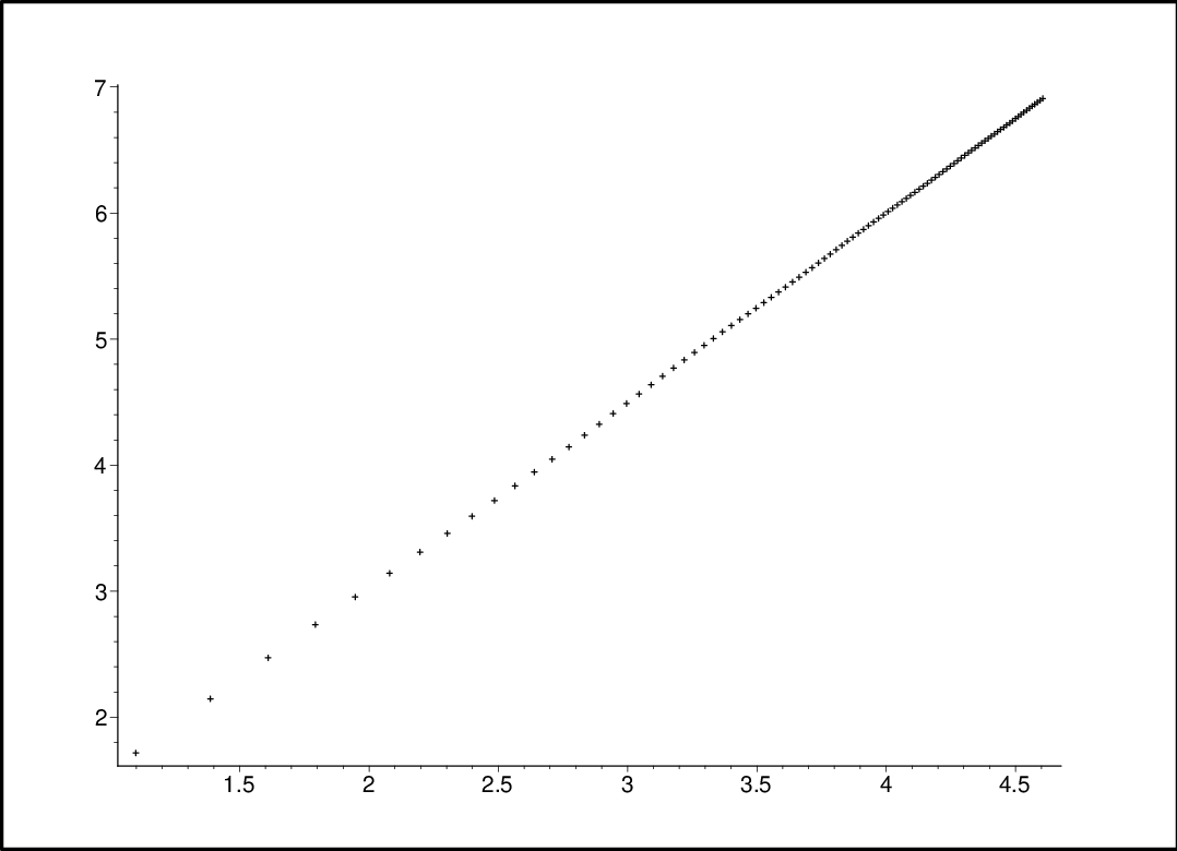
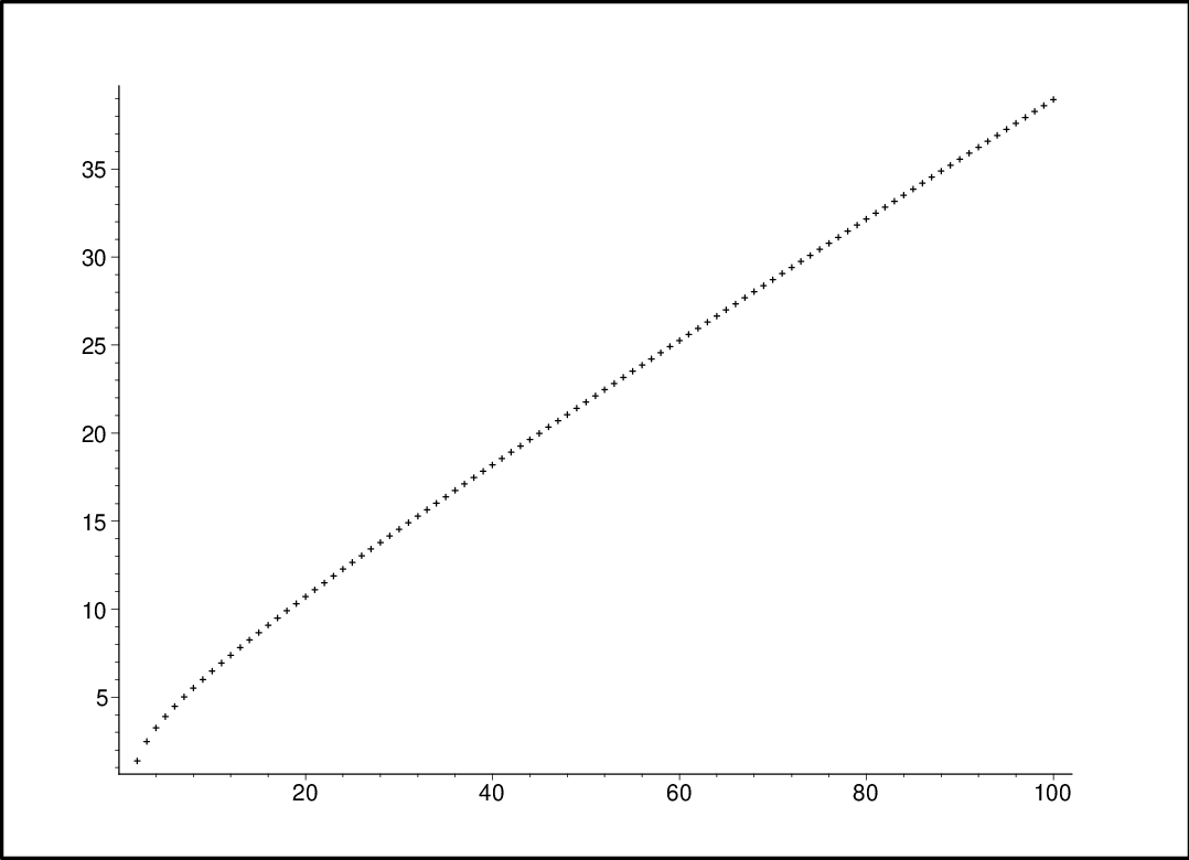
Here we represent the plots of log⁡|JN​(K)|\log|J_{N}(K)| for N=1..100N=1..100, for the hyperbolic knot 414_{1} and for the toric knot 313_{1}.

For the knot 414_{1}, formula (126) for q=e2​π​i/Nq=e^{2\pi i/N} gives

JN​(41)=∑k=1N−1∏j=1k4​sin2⁡π​jN\displaystyle J_{N}(4_{1})=\sum\limits_{k=1}^{N-1}\prod\limits_{j=1}^{k}4\sin^{2}\frac{\pi j}{N} (145)

Note that all the terms in this formula are positive. Using representation (125) and the expansion of quantum dilogarithm function (59) at large NN, this sum might be approximated by the integral

JN​(41)∼∫d​z​exp⁡(N2​π​i​(Li2​(−e−i​z)−Li2​(−ei​z)))\displaystyle J_{N}(4_{1})\sim\int dz\exp\Big(\frac{N}{2\pi i}(\textrm{Li}_{2}(-e^{-iz})-\textrm{Li}_{2}(-e^{iz}))\Big) (146)

Using the saddle point approximation, one obtains

dd​z​(Li2​(−e−i​z)−Li2​(−ei​z))=0⇒log⁡((1+e−i​z)​(1+ei​z))=0⇒ei​z=e2​π​i3\displaystyle\frac{d}{dz}(\textrm{Li}_{2}(-e^{-iz})-\textrm{Li}_{2}(-e^{iz}))=0\Rightarrow\log((1+e^{-iz})(1+e^{iz}))=0\Rightarrow e^{iz}=e^{\frac{2\pi i}{3}} (147)

and for the volume one gets

V​o​l​(41)=−i⁡(Li2​(−e−2​π​i3)−Li2​(−e2​π​i3))≈2.02688\displaystyle Vol(4_{1})=-i\Big(\textrm{Li}_{2}(-e^{-\frac{2\pi i}{3}})-\textrm{Li}_{2}(-e^{\frac{2\pi i}{3}})\Big)\approx 2.02688 (148)

One can directly measure this value as a slope in the plot, Fig.3.

In the case of the toric knot 313_{1}, the quantity JN​(31)J_{N}(3_{1}) may take complex values, and, therefore, the saddle point approximation is more subtle. Fig.4 shows the power behaviour of the absolute value asymptotics which is expected [55] and is consistent with the volume conjecture for the torus knot

|JN​(31)|∼N3/2|J_{N}(3_{1})|\sim N^{3/2}

while the phase of JN​(31)J_{N}(3_{1}) behaves in a much more tricky way [56].
Refer to caption
Figure 3: The plot of ln⁡JN​(41)\ln J_{N}(4_{1}) for N=3​…​100N=3...100. At large NN the plot becomes linear.
Refer to caption
Figure 4: The plot of ln⁡|JN​(31)|\ln|J_{N}(3_{1})| for N=3​…​100N=3...100 as a function of ln⁡N\ln N. At large NN the behavior of the plot is linear with the slope 3/2.

References

  • [1] Yu.Terashima and M.Yamazaki, arXiv:1103.5748
  • [2] D.Gaiotto, arXiv:0904.2715
  • [3] D. Gaiotto, G. Moore, A. Neitzke, arXiv:0907.3987;
    T. Dimofte, S. Gukov, Y. Soibelman, Lett.Math.Phys. 95 (2011) 1-25, arXiv:0912.1346;
    M. Kontsevich and Y. Soibelman, 0811.2435;
    V. Fock and A. Goncharov, Publ. Math. Inst. Hautes Études Sci. 103 (2006) 1-211, math/0311149
  • [4] V.Pestun, arXiv:0906.0638
  • [5] N.Nekrasov and E.Witten, JHEP 1009 (2010) 092, arXiv:1002.0888
  • [6] H.Awata and H.Kanno, arXiv:0910.0083
  • [7] E.Gorsky, arXiv:1003.0916
  • [8] T.Dimofte, S.Gukov and L.Hollands, arXiv:1006.0977
  • [9] R.Dijkgraaf, H.Fuji and M.Manabe, arXiv:1010.4542
  • [10] K. Hosomichi, S. Lee and J. Park, JHEP 1012 (2010) 079, arXiv:1009.0340; JHEP 1103 (2011) 127, arXiv:1012.3512; arXiv:1102.4716
  • [11] E.Witten, arXiv:1001.2933; arXiv:1101.3216
  • [12] F.Dolan, V.Spiridonov and G.Vartanov, arXiv:1104.1787
  • [13] L.Alday, D.Gaiotto and Y.Tachikawa, Lett.Math.Phys. 91 (2010) 167-197, arXiv:0906.3219;
    N.Wyllard, JHEP 0911 (2009) 002, arXiv:0907.2189;
    A.Mironov and A.Morozov, Phys.Lett. B680 (2009) 188-194, arXiv:0908.2190; Nucl.Phys. B825 (2009) 1-37, arXiv:0908.2569
  • [14] K.Hikami, Int.J.Mod.Phys. A16 (2001) 3309-3333, math-ph/0105039; Int.J.Mod.Phys. B16 (2002) 1963-1970; J.Geom.Phys. 57 (2007) 1895-1940, math/0604094;
    T. Dimofte, S. Gukov, J. Lenells, D. Zagier, Commun.Num.Theor.Phys. 3 (2009) 363-443, arXiv:0903.2472
  • [15] R.Poghossian, JHEP 0912 (2009) 038, arXiv:0909.3412;
    V.Alba and And.Morozov, JETP Lett. 90 (2009) 708-712 , arXiv:0911.0363
  • [16] J. Teschner, Int.J.Mod.Phys. A19S2 (2004) 436-458, hep-th/0303150; Contribution to 14th International Congress on Mathematical Physics (ICMP 2003), hep-th/0308031
  • [17] E.W.Barnes, Proc. London Math. Soc. 31 (1899) 358-381; Phil. Trans. Roy. Soc. A196 (1901) 265-387; Trans. Cambr. Phil. Soc. 19 (1904) 374-425
  • [18] T.Shintani, J. Fac. Sci. Univ. Tokyo, Sect. 1A 24 (1977) 167-199;
    N.Kurokawa, Proc. Japan Acad. A67 (1991) 61-64; Proc. Japan Acad. A68 (1992) 256-260; Adv. Studies Pure Math. 21 (1992) 219-226;
    L.Faddeev and R.Kashaev, Mod.Phys.Lett. A9 (1994) 427-434, hep-th/9310070;
    L.Faddeev, Lett. Math. Phys. 34 (1995) 249; hep-th/9504111; math.qa/9912078;
    S.Sergeev, V.Bazhanov, H.Boos, V.Mangazeev and Yu.Stroganov, IHEP-95-129, 1995;
    M.Jimbo and T.Miwa, J.Phys. A29 (1996) 2923-2958; hep-th/9601135;
    S. Ruijsenaars, J. Math. Phys. 38 (1997) 1069–1146;
    R. Kashaev, Lett.Math.Phys. 43 (1998) 105-115
  • [19] E.Witten, Comm.Math.Phys. 121 (1989) 351-399
  • [20] J.Wess and B.Zumino, Phys.Lett. B37 (1971) 95;
    S.Novikov, UMN, 37 (1982) 37;
    E.Witten, Comm.Math.Phys. 92 (1984) 455;
    A.Gerasimov, A.Marshakov, A.Morozov, M.Olshanetsky, S. Shatashvili, Int.J.Mod.Phys. A5 (1990) 2495-2589
  • [21] A.Morozov, Phys.Usp.(UFN) 35 (1992) 671-714; 37 (1994) 1, hep-th/9303139; hep-th/9502091; hep-th/0502010;
    A.Mironov, Int.J.Mod.Phys. A9 (1994) 4355, hep-th/9312212; Phys.Part.Nucl. 33 (2002) 537; hep-th/9409190; hep-th/9409190; Theor.Math.Phys. 114 (1998) 127, q-alg/9711006
  • [22] N.M.Dunfield, S.Gukov and J.Rasmussen, Experimental Math. 15 (2006) 129-159, arXiv:math/0505662
  • [23] S.Gukov, A.Iqbal, C.Kozcaz and C.Vafa, arXiv:0705.1368
  • [24] M. Khovanov, Duke Math. J. 101 (2000) 359-426
  • [25] M. Aganagic, R. Dijkgraaf, A. Klemm, M. Marino, C. Vafa, Commun.Math.Phys. 261 (2006) 451-516, hep-th/0312085;
    M.Marino, Rev.Mod.Phys. 77 (2005) 675-720, hep-th/0405083
  • [26] S.Garoufalidis and T.Le, Geometry and Topology, 9 (2005) 1253-1293, math/0309214
  • [27] A.Alexandrov, A.Mironov and A.Morozov, Int.J.Mod.Phys. A19 (2004) 4127, hep-th/0310113; Teor.Mat.Fiz. 150 (2007) 179-192, hep-th/0605171; Physica D235 (2007) 126-167, hep-th/0608228; JHEP 12 (2009) 053, arXiv:0906.3305;
    A.Alexandrov, A.Mironov, A.Morozov, P.Putrov, Int.J.Mod.Phys. A24 (2009) 4939-4998, arXiv:0811.2825;
    B.Eynard, JHEP 0411 (2004) 031, hep-th/0407261;
    L.Chekhov and B.Eynard, JHEP 0603 (2006) 014, hep-th/0504116; JHEP 0612 (2006) 026, math-ph/0604014;
    N.Orantin, arXiv:0808.0635
  • [28] E. Guadagnini, M. Martellini, M. Mintchev, In ”Clausthal 1989, Proceedings, Quantum groups”, 307-317; Phys.Lett. B235 (1990) 275
  • [29] A.Morozov and A.Smirnov, Nucl.Phys. B835 (2010) 284-313, arXiv:1001.2003
    A.Smirnov, hep-th/0910.5011, to appear in the Proceedings of International School of Subnuclar Phys. in Erice, Italy, 2009
  • [30] V.Drinfeld, Published in ”Problems of modern quantum field theory” 1-13, Alushta, 1989
  • [31] T.T.Q.Le and J. Murakami, Nagoya Math. J.Vol. 142 (1996) 39-65
  • [32] S.Chmutov and S.Duzhin, math/0501040
  • [33] V.Knizhnik and A.Zamolodchikov, Nucl.Phys. B247 (1984) 83-103
  • [34] P. Dunin-Barkovsky, A. Sleptsov and A. Smirnov, to appear
  • [35] S. Chmutov, S. Duzhin, J. Mostovoy, arXiv:1103.5628;
    J.M.F. Labastida, E. Perez, J.Math.Phys. 41 (2000) 2658-2699, hep-th/9807155 J.Math.Phys. 39 (1998) 5183-5198, hep-th/9710176;
    M. Alvarez, J.M.F. Labastida, E. Perez, Nucl.Phys. B488 (1997) 677-718, hep-th/9607030;
    M. Alvarez, J.M.F. Labastida, Commun.Math.Phys. 189 (1997) 641-654, q-alg/9604010; Nucl.Phys. B433 (1995) 555-596, hep-th/9407076
  • [36] Dror Bar-Natan, Edward Witten, Commun.Math.Phys. 141 (1991) 423-440;
    Dror Bar-Natan, Ph.D. Thesis; J.Knot Theor.Ramifications 4 (1995) 503-547; q-alg/9703025;
    R. Kashaev and N.Reshetikhin, math/0202211; math/0202212;
    V.G. Turaev, O.Y. Viro, Topology 31 (1992) 865-902;
    V. G. Turaev, UMN, 41 (247) (1986) 97-147;
    S. Axelrod, I. Singer, Proc. XXth Internat. Conf. on Differential Geometric Methods in Theoretical Physics, arXiv:hep-th/9110056v1
  • [37] M. Goussarov, M. Polyak, O. Viro, Topology, 39(5) (2000) 1045-1068
  • [38] A.Mironov, A.Morozov and S.Natanzon, Theor.Math.Phys. 166 (2011) 1-22, arXiv:0904.4227; arXiv:1012.0433
  • [39] R.Kashaev, arXiv:q-alg/9601025
  • [40] M.Marino, JHEP 0812 (2008) 114, arXiv:0805.3033
  • [41] A.Morozov and Sh.Shakirov, JHEP 0912 (2009) 003 arXiv:0906.003; arXiv:1007.4100
  • [42] W.Turston, The Geometry and Topology of Three-Manifolds, Lecture Notes at Princeton University, 1980
  • [43] R.Gelca, Math. Proc. Cambridge Philos. Soc. 133 (2002) 311-323;
    R. Gelca and J. Sain, J. Knot Theory Ramifications 12 (2003) 187-201
  • [44] S. Garoufalidis and Thao Vuong, arXiv:1010.3147;
    S. Garoufalidis and C. Koutschan, arXiv:1011.6329
  • [45] N.Nekrasov, Nucl.Phys. B531 (1998) 323-344, arXiv:hep-th/9609219;
    A.Gorsky, S.Gukov and A.Mironov, Nucl.Phys., B518 (1998) 689, arXiv:hep-th/9710239;
    A.Marshakov, A.Mironov, Nucl.Phys., B518 (1998) 59-91, arXiv:hep-th/9711156;
    H.W. Braden, A.Marshakov, A.Mironov and A.Morozov, Phys.Lett., B448 (1999) 195, hep-th/9812078; Nucl.Phys., B558 (1999) 371, hep-th/9902205
  • [46] A.Mironov and A.Morozov, JHEP 04 (2010) 040, arXiv:0910.5670; J.Phys. A43 (2010) 195401, arXiv:0911.2396
  • [47] A.Popolitov, arXiv:1001.1407;
    Wei He, Yan-Gang Miao, Phys.Rev. D82 (2010) 025020, arXiv:1006.1214;
    K.Maruyoshi and M.Taki, arXiv:1006.4505;
    A.Marshakov, A.Mironov and A.Morozov, arXiv:1011.4491;
    F.Fucito, J.F.Morales, R.Poghossian and D. Ricci Pacifici, arXiv:1103.4495;
    Y.Zenkevich, arXiv:1103.4843;
    N.Dorey, T.J.Hollowood and S.Lee, arXiv:1103.5726
  • [48] N.Nekrasov and S.Shatashvili, arXiv:0908.4052
  • [49] A.Mironov, A.Morozov, A.Smirnov and Sh.Shakirov, Proving AGT conjecture for β=1\beta=1: extension to five dimensions, to appear
  • [50] S.Kharchev, D.Lebedev and M.Semenov-Tian-Shansky, Commun.Math.Phys. 225 (2002) 573-609, arXiv:hep-th/0007040
  • [51] N.Seiberg and E.Witten, Nucl.Phys., B426 (1994) 19-52, hep-th/9408099; Nucl.Phys., B431 (1994) 484-550, hep-th/9407087;
    A.Gorsky, I.Krichever, A.Marshakov, A.Mironov, A.Morozov, Phys.Lett., B355 (1995) 466-477, hep-th/9505035;
    R.Donagi and E.Witten, Nucl.Phys., B460 (1996) 299-334, hep-th/9510101
  • [52] H.Ooguri and C.Vafa, Nucl.Phys. B577 (2000) 419, hep-th/9912123
  • [53] T. Dimofte, arXiv:1102.4847
  • [54] R. Dijkgraaf and H. Fuji, Fortsch.Phys. 57 (2009) 825-856, arXiv:0903.2084
  • [55] R.Kashaev and O.Tirkkonen, arXiv:math/9912210
  • [56] H.Murakami, Internat. J. Math. 15 (2004) 547-555, arXiv:math/0405126