From individual to collective behaviour of coupled velocity
jump processes: a locust example
Radek Erban11
1
Mathematical Institute,
University of Oxford, 24-29 St. Giles’, Oxford, OX1 3LB, United Kingdom;
e-mail: erban@maths.ox.ac.uk
Jan Haškovec22
2
Johann Radon Institute for Computational
and Applied Mathematics (RICAM), Austrian Academy of Sciences,
Altenbergerstraße 69, A-4040 Linz, Austria;
e-mail: jan.haskovec@oeaw.ac.at
Abstract. A class of stochastic individual-based models, written in terms of coupled velocity jump processes, is presented and analysed. This modelling approach incorporates recent experimental findings on behaviour of locusts. It exhibits nontrivial dynamics with a “phase change” behaviour and recovers the observed group directional switching. Estimates of the expected switching times, in terms of number of individuals and values of the model coefficients, are obtained using the corresponding Fokker-Planck equation. In the limit of large populations, a system of two kinetic equations with nonlocal and nonlinear right hand side is derived and analyzed. The existence of its solutions is proven and the system’s long-time behaviour is investigated. Finally, a first step towards the mean field limit of topological interactions is made by studying the effect of shrinking the interaction radius in the individual-based model when the number of individuals grows.
Key words: Collective behaviour, Stochastic individual-based model, Density-dependent directional switching, Kinetic equation.
1 Introduction
Individual-based behaviour in biology can be often modelled as a velocity jump process [20]. Here, the velocity of an individual is subject to sudden changes (“jumps”) at random instants. If the velocity changes are completely random, this process simply leads to diffusive spreading of individuals in an appropriate limit [18]. The situation becomes more complicated whenever the velocity changes are biased according to an individual’s environment. A classical example is bacterial chemotaxis [8]. Individual bacteria change their frequency of velocity changes according to their environment. If they swim in a favourable direction (e.g. towards a nutrient source), they are less likely to change their direction. On the other hand, they are more likely to turn if they are heading away from a foodstuff [9].
In this paper, we modify the velocity jump methodology to model the behaviour of locusts. Our model is motivated by the recent experiments of Buhl et al [2]. They studied an experimental setting, in which locust nymphs marched in a ring-shaped arena. The collective behaviour depended strongly on locust density. At low densities, there was a low incidence of alignment among individuals. Intermediate densities were characterized by long periods of collective motion in one direction along the arena interrupted by rapid changes of group direction. If the density of locusts was further increased, the group quickly adopted a common and persistent rotational direction. Yates et al [24] analysed experimental data of Buhl et al [2] and proposed that the frequency of random changes in the direction of an individual increases when the individual looses the alignment with the rest of the group. In this paper, we incorporate this observation into a stochastic individual-based model formulated as a velocity jump process. We show that this model, although phenomenologically very simple, has the same predictive power as other modelling approaches previously used in this area [7, 2]. In particular, it exhibits (i) a rapid transition from disordered movement of individuals to highly aligned collective motion as the size of the group grows, and (ii) sudden and rapid switching of the group direction, with frequency decreasing as group size increases.
The individual-based model is introduced in Section 2. The ring-shaped arena, used in Buhl’s experiments [2], is modelled as one-dimensional interval with periodic boundary conditions. Locusts march with a constant speed and each individual switches its direction randomly. The individual switching frequency increases in response to a loss of alignment. In Section 3, the corresponding Fokker-Planck equation is derived for the system with global interactions and possible types of qualitative behaviour of the system are classified. For the case of ordered group motion, where two distinct metastable states exist, an approximate analytic formula for the mean switching time between these two states is derived. Then, in Section 4, the kinetic formulation of the model is obtained in the limit as the number of locusts tends to infinity. The existence of solutions of the kinetic model is shown in Section 5 and the long time behaviour is investigated in Section 6. We conclude with analysis of the dependence of collective behaviour on the size of the interaction radius of the individuals in Section 7.
2 Individual based model
We consider a group of agents (locusts) with time-dependent positions and velocities , . To mimic the ring-shaped arena set-up of [2], we assume that the agents move along a one-dimensional circle, which we identify with the interval with periodic boundary conditions, and move either to the right or to the left with the same unit speed, i.e.
| (2.1) |
We define the local average velocity of the ensemble, seen by the -th agent, as
| (2.2) |
where is a weight function defined on with the properties:
- [A1]
is bounded and nonnegative on ,
- [A2]
.
For example, , where is the characteristic function of the interval and is a interaction radius, satisfies conditions [A1] and [A2]. This is a common choice of in biological applications [7, 24]. It is worth noting that, due to the assumption [A2], the definition (2.2) always makes sense and
The agents switch their velocities to the opposite direction (i.e., from to and vice versa) based on independent Poisson processes with the rates
where and are fixed parameters and the “response to disalignment” function is assumed to be convex, differentiable and symmetric with respect to the origin. Taking the Taylor expansion of around , we obtain
We can set without loss of generality, because it can be absorbed in . Since the individuals switch their velocities less frequently when they are aligned ([24]), has a global minimum at . This implies that . If , we can set by choosing an appropriate time scale. Therefore, has the general form . For the rest of the paper, we choose the form for simplicity. Other choices are certainly possible, for example, in the limiting case the leading order approximation is given by a higher order term, which, however, complicates the analysis. However, it is worth noting that the derivation of the kinetic equation performed in Section 4 is possible, for example, also for , .
With , the turning rate “from the right to the left”, , and the rate for the opposite turn, , are given by
| (2.3) | |||||
| (2.4) |
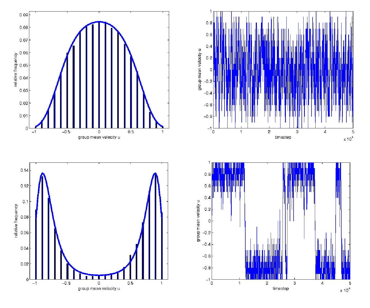
This velocity jump process describes the tendency of the individuals to align their velocities to the average velocity of their neighbors. Despite its relative simplicity, the model provides similar predictions as the Vicsek and Czirók model [7] and its modification [24] and is in qualitative agreement with the experimental observations made in [2]: the transition to ordered motion as grows (Figure 1) and the density-dependent switching behaviour between the ordered states (Figure 2, bottom).

3 Analysis of the individual based model with global interactions
In this section, we simplify the individual-based model by assuming in (2.2), i.e. for all , where
| (3.1) |
where is the number of individuals which are going to the right at time . Using this simplification, we will obtain an explicit formula for the mean switching time between the ordered states. However, for the derivation of the kinetic decription and its analysis (Section 4), we will allow general weights , imposing only the assumption [A1] and a slightly reinforced version of [A2].
Let be the probability that individuals move to the right (i.e., with velocity ) at time . It satisfies the master equation
| (3.2) | |||||
where and are given by (2.3) and (2.4), respectively. The subscript in (2.3)–(2.4) is dropped in (3.2) because all individuals have the same turning rates. Using the system size expansion [23] and the definition (3.1) of the average velocity , we obtain the following Fokker-Planck equation
| (3.3) |
where is the probability distribution function of the average velocity (3.1) at time . The stationary solution of (3.3) is
| (3.4) |
where is the normalization constant and the potential is given by
| (3.5) |
The comparision of the stationary probability distribution function with the results obtained by long-time simulation of the stochastic individual-based model is shown in Figure 2. Differentiating (3.5) twice, we obtain
| (3.6) |
Consequently, we distinguish the following two cases:
- (1)
Large noise: If , then has the global minimum at .
- (2)
Small noise: If , then has a local maximum at . The only local and global minima are at where
It is worth noting that if is small, namely for This is a consequence of approximations made during the derivation of the Fokker-Planck equation (3.3).
In the large noise case, the system prefers the disordered state , while, in the small noise case, the system has two preferred ordered states where it spends most of the time and eventually switches between them (see Figure 2, bottom panel).
Using Kramers theory [15, 13], the mean switching time between the states and can be approximated as
| (3.7) |
which has an exponential asymptotic with respect to large given by
This is in agreement with the experimental observations, [2], as well as with the modified Czirok-Vicsek model of [24], where the mean switching time is as well exponential in . Finally, it is interesting to note that with the transform in (3.7), one has
i.e., if is kept fixed, the mean switching time scales linearly with .
In the numerical experiment shown in Figure 2 bottom (small noise case with , and agents), we have two metastable states located approximately at . The estimate mean turning time given by formula (3.7) is . Performing time steps of length , the observed mean switching time (defined as a mean transition time between the states and or vice versa) was , showing a very good agreement.
4 Kinetic description
In this section we derive the kinetic description of the system of interacting agents and formally pass to the limit to obtain the corresponding kinetic equation. For this, we have to accept a slight reinforcement of the assumption [A2] on , namely,
- [A2’]
on the interval for some .
The state of the system of agents at time is described by the probability density function of finding the -th agent in position with velocity , for . When convenient, we will use the abbreviation , with and . The probability density evolves according to
| (4.1) |
where (resp. ) is the loss (resp. gain) term corresponding to the velocity jumps. Using (2.3)–(2.4), the rate of the switch is for given by
where is defined by (2.2), i.e. is the local average velocity seen by an agent located at , based on the system configuration . Consequently, the loss term is given by
| (4.2) |
We define the operator for and by
| (4.3) |
i.e. denotes the velocity vector created from by changing the sign of its -th component. Then the gain term is given by
| (4.4) |
where
Consequently, the right hand side of (4.1) is
| (4.5) | |||||
where we dropped the dependance on time to simplify the notation. Finally, we postulate the so-called indistinguishability-of-particles: We only consider solutions that are indifferent to permutations of their -arguments. Such solutions are admissible, since the equation (4.1) with the collision operator (4.5) is as well indifferent with respect to interchange of the -pairs.
4.1 Derivation of the BBGKY hierarchy
To derive an analogue of what is called the BBGKY hierarchy in the classical kinetic theory of gases (see, for instance, [6]), we define, for , the -agent marginals
| (4.6) |
In what follows, the coordinates of and will be denoted as
that is, . The same notational convention is used for velocities, i.e., . Note that, due to the indistinguishability-of-particles, the marginals are well defined and indifferent with respect to permutations of the pairs of arguments , . Integrating (4.1), we obtain
| (4.7) |
Substituting (4.5) into the right-hand side of (4.7), we get
| (4.8) | |||||
Since we are interested in the limit with fixed, we can rewrite the definition (2.2) as follows
| (4.9) | |||||
where we define
Substituting (4.9) in (4.8) and (4.7), we obtain the BBGKY hierarchy
| (4.10) | |||||
where
| (4.11) |
and
| (4.12) |
4.2 Passage to the limit
The usual procedure of deriving the mean field equation is to write the BBGKY hierarchy (4.10) in terms of and pass to the limit to obtain the so-called Boltzmann hierarchy for [22]. Then, one shows that the Boltzmann hierarchy admits solutions generated by the molecular chaos ansatz (see below). In our case, however, this strategy cannot be pursued; although we could derive uniform estimates allowing us to pass to the limit in the BBGKY hierarchy, we are not able to express the limiting marginals and in terms of . Consequently, we have no clue what the correct molecular chaos ansatz for and should be.
Instead, we assume the propagation of chaos already at the level of the BBGKY hierarchy, before passing to the limit : we assume that, for large , is well approximated by the product of the limiting one-particle marginals , i.e.
| (4.13) |
This corresponds to vanishing statistical dependence (correlations) between the agents as and is the usual phenomenon observed in systems of interacting particles, see for instance [6] in the context of classical kinetic theory or [16, 17] in the context of biological systems. Moreover, if one interprets (resp. ) as the first (resp. second) order moment of with respect to , then one can understand (4.13) as the moment closure assumption for the non-closed system of moments generated by (4.1).
The essential point is that now we may insert (4.13) into (4.11) and (4.12) to obtain explicit expressions for and in terms of :
| (4.14) | |||
and
| (4.15) | |||
Study of the limit in (4.14) and (4.15)
We start by setting , which is the case considered in Section 4.3. To simplify the notation, we drop the bars over and , and, without loss of generality, choose . First, we explore the symmetry of the expression (4.14) as follows:
with the notation
and
| (4.16) |
Due to the normalization of , we have . Consequently, in what follows we denote by the time dependent probability measure corresponding to the probability density . Since is bounded and nonnegative by assumption [A1], it is integrable with respect to and we may define
| (4.17) |
The forthcoming analysis will be performed given the assumption ; the case will be discussed in Remark 2.
Lemma 1
Let be a probability measure on with density and such that . Let with be such that the integral defined by is positive. Define
Then
Proof: We can treat as a random variable with respect to the probability measure . The essential tool of the proof is the law of large numbers, which states that converges to in measure, in the sense that for each ,
| (4.18) |
where denotes the -fold tensor product of the probability measures . Moreover, the existence of the -th order moment of with respect to ,
implies the rate of convergence (see [1])
| (4.19) |
Let us denote by the set and by its complement in . Choosing and , we have the estimate
Consequently,
On the other hand, the integral over is estimated with
The first term on the right hand side converges to zero as by (4.18) and the boundedness of . Using (4.16), the second term is estimated by
and vanishes as due to (4.19) with . Consequently, we have shown that the term
can be made arbitrarily small, for sufficiently large .
The formula (4.15) can be analysed in a similar way as we did for (4.14). Namely, we exploit its symmetry as follows,
| (4.20) | |||||
The limiting behaviour of the first term is studied in the following Lemma:
Lemma 2
Proof: We follow the lines of the proof of Lemma 1. Defining again and , with , we derive the estimates
and
where the first term vanishes in the limit due to (4.18) and the second one by (4.19) with .
4.3 Derivation of kinetic and hydrodynamic description
Let us denote and . We define , the continuous analogue of the local average velocity (2.2), by
| (4.22) |
where
We extend the definition of to the whole domain by setting for , see Remark 2.
The kinetic equation for is obtained by setting in the BBGKY-hierarchy (4.10) with the molecular chaos assumption (4.13) and passing to the limit . Using Lemma 1 and formula (4.21), we obtain
| (4.23) |
Consequently, (4.10) reduces to the following system of two equations
| (4.24) | |||||
| (4.25) |
Equivalently, defining the mass density and flux by
| (4.26) |
the system can be written in the hydrodynamic description as
| (4.27) | |||||
| (4.28) | |||||
with
Remark 2
Due to the assumption [A2’], we have on . Therefore, both in and in are equal to zero by definition. Consequently,
and formulas remain valid irrespective of the particular choice of the value of . This justifies our extension of the definition of by setting it equal to zero for .
5 Existence of solutions to the kinetic system
The main goal of this Section is to prove the following Theorem:
Theorem 1
Proof of Theorem 1: The proof is carried out in three steps and is only sketched here, omitting details where the techniques are standard. For notational convenience, we will work both with the kinetic and hydrodynamic representation of the system and treat and as synonyms, related by (4.26).
Step 1. First, we consider a linearized version of (4.24)–(4.25), where we solve for and given a prescribed with . This constitutes a strictly hyperbolic system with unique mild, nonnegative solution in , constructed by a standard fixed point iteration (see, for instance, [10], Section 7.3). The solution is given by the Duhamel formula
| (5.1) | |||||
| (5.2) |
with . Moreover, for any fixed , we have apriori boundedness of and in , depending only on the initial condition. Indeed, denoting , and remembering the uniform boundedness , we have
and the apriori boundedness follows from an application of the Gronwall lemma on the time interval .
Step 2. We consider a regularized version of (4.24)–(4.25) where is substituted by , defined by
| (5.3) |
For any fixed , a solution is found by the Schauder fixed point iteration on the mean velocity [10]. The compactness of the corresponding Schauder operator is provided by the Arzela-Ascoli theorem. Indeed, let us take a sequence with and let and be the corresponding mild solutions of the kinetic system, given by the Duhamel formula (5.1)–(5.2) with in place of , and let and . As explained in Step 1, for any fixed we have , bounded uniformly with respect to . Defining the function
one has (continuity of translation [21]). By Hölder inequality,
with . Moreover, we have the uniform boundedness
and analogous estimates hold for . Consequently, we have
This uniform equicontinuity together with the uniform boundedness allows us to apply the Arzela-Ascoli Lemma and obtain the compactness of the Schauder operator. Therefore, for every fixed , we have a nonnegative solution of the regularized system (4.24), (4.25), (5.3), uniformly bounded (with respect to ) in .
Step 3. Finally, we pass to the limit . Due to the uniform boundedness, a subsequence of weakly* in ; we need to show that the limit of the nonlinear terms and is and, resp., , with given by (4.22), or, equivalently, (4.3). The limit passage in the distributional formulation of the term with a test function is performed as follows:
The first term vanishes in the limit due to the weak* convergence of towards with a valid test function. Concerning the second term, we will show that tends to zero for almost all and conclude the convergence of the time integral by the Lebesgue dominated convergence theorem. Let us fix and define the set by
with and defined in (5.3). Then, we have
where the second line is due to on and because tends to zero as . Next, for ,
where and . Therefore, due to the uniform convergence of and to and, resp., on (implied by the uniform equicontinuity and boundedness of the families and ), we have
We conclude by passing . The limit passage in the term is performed similarly (note that ).
It is worth noting that the assumption [A1] of Theorem 1 can be relaxed. In fact, we posed the requirement [A1] of boundedness of on in order to establish the definition (2.2) of in the discrete model and pass to the limit . However, at the level of the kinetic or hydrodynamic description, we may relax this to . Moreover, formally it is possible to consider even singular weights, in particular , which leads to and removes the nonlocality. In fact, one can see the choice as the limiting case when the interaction radius shrinks to zero: for almost all such that , one has
where is the characteristic function of the interval . One can interpret this as a model where only pointwise local observations of the system are possible.
By a slight modification of the proof of Theorem 1 it is possible to show that given a sequence of weights converging strongly in to , the solutions corresponding to the weights converge weakly* in to the solution corresponding to the weight . However, we need the condition [A2’] to be satisfied uniformly; consequently, the question whether and how the solution corresponding to can be obtained as a limit of solutions with as remains an interesting open problem. An even more interesting question is what is the limit of the discrete model as if the interaction radius is shrinking as some power of . This question is studied in Section 7 below.
6 Long time behaviour
In this Section we provide several conjectures about the long time behaviour of the kinetic system (4.22), (4.24), (4.25) or, equivalently, the hydrodynamic system (4.27)–(4.3). To get some insight into the long time dynamics, we start with a numerical example. We solve the kinetic system using standard semi-implicit finite difference method with upwinding. The initial condition is on and zero otherwise, on and zero otherwise. In Figure 3 we show the results for the choice of parameters and and the weight function .

|

|

|

|

|

|

|

|

|

|

|

|
We conjecture that with regular weights satisfying [A1] and [A2’], the solutions to (4.27)–(4.3) converge to the constants and with some , exponentially fast as . Moreover, in the large noise case , we hypothesize that . Unfortunately, we are only able to provide an analytical proof in the rather special case and :
Lemma 3
Assuming , we have , where satisfies the ordinary differential equation
| (6.1) |
subject to the initial condition . Moreover,
- (i)
if , then ,
- (ii)
if , then and
(6.2) Moreover, converges to zero exponentially fast in the -sense:
for a suitable constant .
Proof: Integrating (4.28) with with respect to , we obtain (6.1). This has the stationary state , which is stable if and only if . Moreover, if , two additional stable stationary states exist. This establishes the first statement. Further, we have
and an application of the Gronwall lemma gives (6.2).
To prove the convergence of to zero, we consider the identity
| (6.3) |
An application of the Cauchy-Schwartz inequality and the decay rate (6.2) yield
Then, an integration of (6.3) in time leads to
with . Consequently, by the Gronwall lemma, is bounded uniformly in time by a constant if . Inserting this information into (6.3) gives
and an application of the Gronwall lemma yields the second statement.
6.1 The case
In this subsection we briefly discuss the long time behaviour in the singular case . Again, we start with a numerical example where we solve the kinetic system with the parameters and . The initial condition is chosen as before, see Figure 3 (left panels). In Figure 4 we present the time evolution of , , , and . Based on the numerical observations, we conjecture that, for the small noise case , the long time dynamics are given by the travelling wave profiles , satisfying
and with . Then, it is a matter of a simple consideration to deduce that one of the functions, say , has to be a global constant, while the other one, , is a piecewise constant assuming only two values , satisfying the relations
These relations chracterize the dynamic equilibria between the densities of individuals marching to the left and to the right, in dependence on the parameter values and .

|

|

|

|

|

|

|

|

|

|

|

|
For the large noise case (), we prove that the asymptotic state is again and . In fact, converges to in the -sense exponentially fast as . This follows from an application of the Gronwall lemma to the estimate
7 The effect of shrinking interaction radius
In biological applications, the weight function is often chosen as the characteristic function of the interval , where is the interaction radius. It is important to study the dependence of collective behaviour on the size of . In this section, we will consider a theoretical limit . Clearly, letting with fixed leads to a trivial model without any interactions (it corresponds to the choice ). On the other hand, letting first , followed by , we obtain the model with , as mentioned in Section 5. Consequently, the limits and do not commute. From the modelling point of view, it is natural to study the limit with the interaction radius shrinking as for some . Indeed, as the space is getting more crowded, the visibility is reduced and every individual can only take into account its closest neighbours. Actually, taking and letting , we will show that a significant limit is obtained with , leading to a new kinetic model. The results are summarized in the following Theorem.
Theorem 2
Let . Then, the formal limit as of the BBGKY hierarchy is
- (1)
For :
(7.1) - (2)
For :
(7.2) (7.3) - (3)
For :
(7.4) (7.5) with
(7.6) where is the so-called exponential integral function and is Euler’s constant.
We see that for , we obtained the kinetic model with (i.e., the same as if one would first pass to and then ). If , we get the model with no interactions (i.e., as if one would first pass to and then ) which is described by the telegraph equation for [19]. In the significant limit with we obtained a new model, which is in fact the hydrodynamic model (4.27)–(4.28) with the function in place of and with , given by (7.6), in place of .
Proof: All we need to do is to recalculate the limits in the expressions (4.11) and (4.12) with . Let us fix and assume that it is a Lebesgue point of and , i.e.,
| (7.7) |
and similarly for . Moreover, assume that . In the same way as in Lemma 1, we calculate
where we denoted
Obviously, the sum only takes the values , and
Therefore,
Due to (7.7), we have and . Therefore,
and
Using the same technique as above, one calculates that
with
It is easily shown that vanishes in the limit whenever , while with the law of rare events ([11]) gives
We assume that and be integrable functions, so that almost every is a Lebesgue point for them.
Remark 3
Our analysis can be seen as a first step towards a so-called topological model, where the agent interactions are based on some connectivity graphs. For instance, one can consider the situation where every agent interacts only with its nearest neighbour. In this case, we have a different time dependent weight function for every agent, namely with . Then, the passage to the corresponding continuum model is a completely open problem; however, let us observe that
Therefore, it would be interesting to consider the discrete system with ,
| (7.9) |
and study the limit and (possibly with ). Moreover, let us observe that “on average”, . Therefore,
so we are in the situation of the significant limit described above, and we might believe that the new kinetic model obtained in this limit can have some connection with the limit and of .
8 Discussion
We introduced an individual based model with velocity jumps aimed at explaining the experimentally observed collective motion of locusts marching in a ring shaped arena [2]. The frequency of individual velocity jumps increases with a local or global loss of group alignment. We showed that our model has the same predictive power as the model of Czirók and Vicsek, in particular, it exhibits the rapid transition to highly aligned collective motion as the size of the group grows and the switching of the group direction, with frequency rapidly decreasing with increasing group size. Moreover, in the limit we obtained a system of two kinetic equations. We proved existence of its solutions and a partial result about the long time behaviour. Finally, we studied the effect of shrinking the interaction radius in the discrete model as the number of individuals, , tends to infinity. We showed that in the significant limit where shrinks as , one obtains a new kinetic model.
Kinetic approach has previously been used in the literature to understand collective dynamics of individual based models. Carrillo et al [3] found the double milling phenomena in the kinetic formulation of the model of self propeled particles with three zones of interactions. The kinetic description of the Cucker-Smale model was introduced in [14], which can also be be derived from the Boltzmann-type equation, see [4], or Povzner-type equation, [12]. For the survey of the most recent results see the review [5].
Several interesting questions remain open, offering space for future investigations. For example, the kinetic system (4.24)–(4.25) deserves a better analysis, in particular, uniqueness of solutions and more complete investigation of the long time behaviour. It would also be interesting to know if and how the solutions corresponding to can be derived as a limit of solutions corresponding to as . Another interesting direction of future research was formulated in Remark 3.
Acknowledgment: This publication was based on work supported by Award No. KUK-C1-013-04, made by King Abdullah University of Science and Technology (KAUST). JH acknowledges the financial support provided by the FWF project Y 432-N15 (START-Preis “Sparse Approximation and Optimization in High Dimensions”). The research leading to these results has received funding from the European Research Council under the European Community’s Seventh Framework Programme (FP7/2007-2013)/ ERC grant agreement no 239870. RE would also like to thank Somerville College, University of Oxford, for a Fulford Junior Research Fellowship. Both authors would like to thank to the Isaac Newton Institute for Mathematical Sciences in Cambridge (UK), where they worked together during the program “Partial Differential Equations in Kinetic Theories”. The authors also acknowledge several interesting discussions and valuable hints provided by Jan Vybíral of the Johann Radon Institute for Computational and Applied Mathematics (RICAM), Austrian Academy of Sciences, and Christian Schmeiser of the Faculty of Mathematics, University of Vienna.
References
- [1] L. Baum and M. Katz, Convergence rates in the law of large numbers, Transactions of the American Mathematical Society, 120 (1965), pp. 108–123.
- [2] J. Buhl, D. Sumpter, I. Couzin, J. Hale, E. Despland, E. Miller, and S. Simpson, From disorder to order in marching locusts, Science, 312 (2006), pp. 1402–1406.
- [3] J. Carrillo, M. D’Orsogna, and V. Panferov, Double milling in self-propelled swarms from kinetic theory, Kinetic and Related Models, 2 (2009), pp. 363–378.
- [4] J. Carrillo, M. Fornasier, J. Rosado, and G. Toscani, Asymptotic flocking dynamics for the kinetic cucker–smale model, SIAM Journal on Mathematical Analysis, 42 (2010), pp. 218–236.
- [5] J. Carrillo, M. Fornasier, G. Toscani, and F. Vecil, Particle, kinetic, hydrodynamic models of swarming, in Mathematical Modeling of Collective Behavior in Socio-Economic and Life Sciences, G. Naldi, L. Pareschi, and G. Toscani, eds., Modelling and Simulation in Science and Technology, Birkhäuser, 2010, pp. 297–336.
- [6] C. Cercignani, R. Illner, and M. Pulvirenti, The Mathematical Theory of Dilute Gases, Applied Mathematical Sciences, 106, Springer-Verlag, 1994.
- [7] A. Czirók, A. Barabási, and T. Vicsek, Collective motion of self-propelled particles: Kinetic phase transition in one dimension, Physical Review Letters, 82 (1999), pp. 209–212.
- [8] R. Erban and H. Othmer, From individual to collective behaviour in bacterial chemotaxis, SIAM Journal on Applied Mathematics, 65 (2004), pp. 361–391.
- [9] , From signal transduction to spatial pattern formation in E. coli: A paradigm for multi-scale modeling in biology, Multiscale Modeling and Simulation, 3 (2005), pp. 362–394.
- [10] L. Evans, Partial Differential Equations, American Mathematical Society, Providence, Rhode Island, 1998.
- [11] W. Feller, An introduction to probability theory and its applications, Viley, New York, Sydney, 3 ed., 1967.
- [12] M. Fornasier, J. Haskovec, and G. Toscani, Fluid dynamic description of flocking via the povzner-boltzmann equation, Physica D: Nonlinear Phenomena, 240 (2011), pp. 21 – 31.
- [13] D. Gillespie, Markov Processes, an introduction for physical scientists, Academic Press, Inc., Harcourt Brace Jovanowich, 1992.
- [14] S. Ha and E. Tadmor, From particle to kinetic and hydrodynamic descriptions of flocking, Kinetic and Related Models, 1 (2008), pp. 415–435.
- [15] P. Hänggi, P. Talkner, and M. Borkovec, Reaction-rate theory: fifty years after Kramers, Reviews of Modern Physics, 62 (1990), pp. 251–341.
- [16] J. Haškovec and C. Schmeiser, Stochastic particle approximation for measure valued solutions of the 2d Keller-Segel system, Journal of Statistical Physics, 135 (2009), pp. 133–151.
- [17] , Convergence analysis of a stochastic particle approximation for measure valued solutions of the 2d Keller-Segel system. available as http://homepage.univie.ac.at/christian.schmeiser/kellersegel-article2.pdf, 2010.
- [18] T. Hillen and H. Othmer, The diffusion limit of transport equation derived from velocity-jump processes, SIAM Journal on Applied Mathematics, 61 (2000), pp. 751–775.
- [19] M. Kac, A stochastic model related to the telegrapher’s equation, Rocky Mountain Journal of Mathematics, 4 (1974), pp. 497–509.
- [20] H. Othmer, S. Dunbar, and W. Alt, Models of dispersal in biological systems, Journal of Mathematical Biology, 26 (1988), pp. 263–298.
- [21] W. Rudin, Functional Analysis, McGraw-Hill Science, 1991.
- [22] A. Sznitman, Topics in Propagation of Chaos, Lecture notes in mathematics, vol. 1464, Springer-Verlag, 1991.
- [23] N. van Kampen, Stochastic Processes in Physics and Chemistry, North-Holland, Amsterdam, 3rd ed., 2007.
- [24] C. Yates, R. Erban, C. Escudero, I. Couzin, J. Buhl, I. Kevrekidis, P. Maini, and D. Sumpter, Inherent noise can facilitate coherence in collective swarm motion, Proceedings of the National Academy of Sciences USA, 106 (2009), pp. 5464–5469.