Flux representation of an effective

Polyakov loop model for QCD thermodynamics

Christof Gattringer

Institut für Physik, Karl-Franzens-Unversität Graz

Universitätsplatz 5, 8010 Graz, Austria

To appear in Nuclear Physics B.

Introductory remarks

With the running and upcoming experiments at BNL, CERN, GSI and Dubna the amount of experimental facts about the QCD phase diagram will increase considerably in the near future. Also the theoretical side is challenged to contribute to our understanding of QCD thermodynamics, a task which is rather demanding due to the non-perturbative nature of the problem. In principle lattice QCD is a suitable non-perturbative approach, but at finite chemical potential the complex phase problem considerably limits the applicability of Monte Carlo methods for a numerical evaluation of the path integral.

A tempting idea to overcome the complex phase problem is to search for a transformation to new degrees of freedom where the partition function becomes a sum over configurations with real and positive weights. Such representations with real and positive weights can then be used in a Monte Carlo calculation. Several examples for this kind of transformations in various models can be found in the literature, but for QCD we are still far from identifying suitable degrees of freedom.

In this article we contribute to the enterprise of developing new and real representations for QCD related systems with a quark chemical potential $\mu$ by considering an effective theory for Polyakov loop variables. The Polyakov loop has the interpretation of a static color source and in pure gauge theory its expectation value serves as an order parameter for the deconfinement transition. More specifically it is an order parameter for center symmetry which is broken spontaneously at the deconfinement transition of pure gauge theory. Although in full QCD the underlying center symmetry is broken explicitly by the quarks, also there the Polyakov loop may be used to determine the crossover to deconfinement.

The idea of using effective theories for the Polyakov loop to describe the transitions in pure gluodynamics and in QCD goes back to the late seventies, and since then, both the understanding of sub-leading terms in the effective action, as well as the simulation techniques have been improved considerably [1]–[10].

The effective theory for the Polyakov loop considered here may be derived from QCD using strong coupling expansion for the gauge action and hopping expansion for the fermion determinant. The leading center symmetric and center symmetry breaking terms are taken into account, as well as the chemical potential $\mu$ . For $\mu\neq 0$ the action becomes complex, i.e., in its standard representation the theory inherits the complex phase problem from QCD.

In this work we apply high temperature expansion techniques and derive a flux representation which is free of the complex phase problem. The new degrees of freedom are integer valued flux variables attached to the links of the lattice and integer valued monomer variables at the sites. The flux-monomer configurations are subject to constraints which enforce the total flux at each site to be a multiple of three. The weight factors for the admissible configurations are given in closed form and turn out to be real and positive. Thus, in the flux representation a Monte Carlo simulation of the system with generalized Prokof’ev-Svistunov worm algorithms [11] becomes possible and should allow for an effective numerical treatment without any complex phase problems. Finally, we show how observables can be expressed in terms of the flux and monomer variables.

The effective theory and its high temperature expansion

The effective Polyakov loop theory we consider is described by the action

	$\displaystyle S[P]$	$\displaystyle\;=\;$	$\displaystyle-\,\tau\sum_{x}\sum_{\nu=1}^{3}\Big[\,\mathrm{Tr}\,P(x)\,\mathrm{Tr}\,P(x\!+\!\hat{\nu})^{\dagger}\,+\,\mathrm{Tr}\,P(x)^{\dagger}\,\mathrm{Tr}\,P(x\!+\!\hat{\nu})\,\Big]$		(1)
			$\displaystyle-\,\sum_{x}\Big[\,\eta\,\mathrm{Tr}\,P(x)\,+\,\overline{\eta}\;\mathrm{Tr}\,P(x)^{\dagger}\,\Big]\;.$		(1)

In this standard representation the degrees of freedom are the SU(3) valued Polyakov variables $P(x)$ attached to the sites $x$ of a three-dimensional cubic lattice which we consider to be finite with periodic boundary conditions. By $\hat{\nu}$ we denote the unit vector in $\nu$ -direction, with $\nu=1,2,3$ . The first term of the action, which may be obtained from a strong coupling expansion, is a nearest neighbor interaction of the traced Polyakov loops. This expansion also establishes $\tau$ to be an increasing function of the QCD temperature, and for simplicity we refer to $\tau$ as temperature. The term in the second line of (1) can be derived from the fermion determinant using hopping expansion. The parameters $\eta$ and $\overline{\eta}$ are related to the amplitude $\kappa$ and the chemical potential $\mu$ via

\eta\;=\;\kappa\,e^{\,\mu}\quad,\qquad\overline{\eta}\;=\;\kappa\,e^{-\mu}\;.

(2)

The hopping expansion identifies $\kappa$ to be proportional to a power of the hopping parameter and thus $\kappa$ is a function of the quark mass $m$ which decreases with increasing $m$ . For $N_{f}$ flavors of mass degenerate quarks $\kappa$ is simply proportional to $N_{f}$ . The terms $e^{\mu}\,\mathrm{Tr}\,P(x),\,e^{-\mu}\,\mathrm{Tr}\,P(x)^{\dagger}$ in (1), (2) are the leading $\mu$ -dependent terms of the fermion determinant¹¹ 1 Actually in the fermion determinant the chemical potential appears rescaled with the temporal extent $N_{t}$ of the lattice, but in order to simplify the notation used for the effective theory we omit this factor..

From Eq. (1) one immediately sees that the effective theory has a complex phase problem: For $\mu\neq 0$ one has $\eta\neq\overline{\eta}$ , which leads to a non-vanishing imaginary contribution to the action given by $i\sum_{x}(\overline{\eta}-\eta)\,\mathrm{Im}\,P(x)$ . Thus the Boltzmann factor $\exp(-S[P])$ obtains a complex phase and cannot be used as a probability weight in a Monte Carlo calculation.

Effective theories of the type (1) were studied before in various contexts. For the case of vanishing $\kappa$ an important line of research is the determination of sub-leading terms in the action to get the effective theory ready for quantitative analysis – see, e.g., [7]–[8]. For the case of non-zero chemical potential an important contribution is [10], where the theory described by (1) was studied with complex Langevin techniques. A future numerical simulation with the flux representation presented here should be able to check the results [10] and shed light on the reliability of the complex Langevin method.

A reduced version of the model (1), where the traced Polyakov loops are replaced by center elements, was studied as well [3]–[6]. In this simpler case a flux representation free of complex phases has been known for a long time [3] and various numerical simulations with different techniques were presented [3]–[6].

The grand canonical partition function of the model described by (1) is obtained by integrating the Boltzmann factor $e^{-S[P]}$ over all configurations of the Polyakov loop variables. The corresponding measure is a product over the reduced Haar measures $dP(x)$ at the sites $x$ . Thus

Z\;=\;\int\!\prod_{x}dP(x)\;e^{-S[P]}\;=\;\int\!D[P]\;e^{-S[P]}\;,

(3)

where in the second step we have introduced the shorthand notation $D[P]=\prod_{x}dP(x)$ for the product measure.

The first steps towards the flux representation are writing the Boltzmann factors in a factorized form and an expansion of the remaining exponentials. This step corresponds to an expansion in $\tau$ . In spin system language $\tau$ would have to be identified with the inverse temperature $\beta$ and thus our expansion is equivalent to high temperature expansion in statistical mechanics. We obtain the following form of the partition sum:

$\displaystyle Z\!\!$	$\displaystyle\!\!=\!\!\!$	$\displaystyle\!\!\int\!\!D[P]\!\left(\prod_{x,\nu}e^{\tau\,\mathrm{Tr}\,P(x)\,\mathrm{Tr}\,P(x+\hat{\nu})^{\dagger}}\,e^{\tau\,\mathrm{Tr}\,P(x)^{\dagger}\,\mathrm{Tr}\,P(x+\hat{\nu})}\!\right)\!\!\!\left(\prod_{x}e^{\eta\,\mathrm{Tr}\,P(x)}\,e^{\overline{\eta}\,\mathrm{Tr}\,P(x)^{\dagger}}\!\right)$	(4)
	$\displaystyle\!\!=\!\!\!$	$\displaystyle\!\!\int\!\!D[P]\!\left(\prod_{x,\nu}\left[\sum_{l_{x,\nu}=0}^{\infty}\frac{\tau^{l_{x,\nu}}}{l_{x,\nu}!}\Big(\mathrm{Tr}\,P(x)\Big)^{l_{x,\nu}}\Big(\mathrm{Tr}\,P(x+\hat{\nu})^{\dagger}\Big)^{l_{x,\nu}}\right]\right)$
		$\displaystyle\hskip 17.07164pt\times\left(\prod_{x,\nu}\left[\sum_{\overline{l}_{x,\nu}=0}^{\infty}\frac{\tau^{\overline{l}_{x,\nu}}}{\overline{l}_{x,\nu}!}\Big(\mathrm{Tr}\,P(x)^{\dagger}\Big)^{\overline{l}_{x,\nu}}\Big(\mathrm{Tr}\,P(x+\hat{\nu})\Big)^{\overline{l}_{x,\nu}}\right]\right)$
		$\displaystyle\times\Bigg(\prod_{x}\Bigg[\sum_{s_{x}=0}^{\infty}\frac{\eta^{s_{x}}}{s_{x}!}\Big(\mathrm{Tr}\,P(x)\Big)^{s_{x}}\Bigg]\Bigg)\Bigg(\prod_{x}\Bigg[\sum_{\overline{s}_{x}=0}^{\infty}\frac{\overline{\eta}^{\overline{s}_{x}}}{\overline{s}_{x}!}\Big(\mathrm{Tr}\,P(x)^{\dagger}\Big)^{\overline{s}_{x}}\Bigg]\Bigg)\;.$

In the end the partition function will be a sum over configurations of the expansion coefficients $l_{x,\nu},\overline{l}_{x,\nu}$ for the nearest neighbor terms, and the expansion coefficients $s_{x},\overline{s}_{x}$ for the site terms. We will refer to $l_{x,\nu},\overline{l}_{x,\nu}$ as flux variables and to $s_{x},\overline{s}_{x}$ as monomer variables. For the sum over flux- and monomer configurations we introduce the shorthand notation

\sum_{\{l,\overline{l},s,\overline{s}\}}\;=\;\left(\prod_{x,\nu}\;\sum_{l_{x,\nu}=0}^{\infty}\;\sum_{\overline{l}_{x,\nu}=0}^{\infty}\,\right)\left(\prod_{x}\sum_{s_{x}=0}^{\infty}\;\sum_{\overline{s}_{x}=0}^{\infty}\,\right)\;.

(5)

Using this notation, rearranging the products in (4), and writing the integral over all configurations of the Polyakov loops $P(x)$ again in its factorized form, the partition sum reads

$\displaystyle Z\!$	$\displaystyle\!\!=\!\!$	$\displaystyle\!\!\!\sum_{\{l,\overline{l},s,\overline{s}\}}\!\left(\prod_{x,\nu}\;\frac{\tau^{l_{x,\nu}+\overline{l}_{x,\nu}}}{l_{x,\nu}!\;\overline{l}_{x,\nu}!}\right)\left(\prod_{x}\;\frac{\eta^{s_{x}}\;\overline{\eta}^{\overline{s}_{x}}}{s_{x}!\;\overline{s}_{x}!}\right)$	(6)
		$\displaystyle\!\!\times\!\left(\!\prod_{x}\int\!\!dP(x)\,\Big(\mathrm{Tr}\,P(x)\Big)^{\sum_{\nu}[l_{x,\nu}+\overline{l}_{x-\hat{\nu},\nu}]+s_{x}}\Big(\mathrm{Tr}\,P(x)^{\dagger}\Big)^{\sum_{\nu}[\overline{l}_{x,\nu}+l_{x-\hat{\nu},\nu}]+\overline{s}_{x}}\right)$
	$\displaystyle\!\!=\!\!$	$\displaystyle\!\!\!\sum_{\{l,\overline{l},s,\overline{s}\}}\!\!W[l,\overline{l},s,\overline{s}]\;\prod_{x}\,{I}\bigg(\sum_{\nu}[l_{x,\nu}+\overline{l}_{x-\hat{\nu},\nu}]+s_{x}\bigg\|\sum_{\nu}[\overline{l}_{x,\nu}+l_{x-\hat{\nu},\nu}]+\overline{s}_{x}\bigg)\;.$

In the last step we introduced the weight factor for a configuration of flux- and monomer variables,

W[l,\overline{l},s,\overline{s}]\;=\;\left(\prod_{x,\nu}\;\frac{\tau^{l_{x,\nu}+\overline{l}_{x,\nu}}}{l_{x,\nu}!\;\overline{l}_{x,\nu}!}\right)\left(\prod_{x}\;\frac{\eta^{s_{x}}\;\overline{\eta}^{\overline{s}_{x}}}{s_{x}!\;\overline{s}_{x}!}\right)\;,

(7)

and for the remaining SU(3) integrals at the sites use the abbreviation

{I}(n|m)\;=\;\int dP\,\Big(\mathrm{Tr}\,P\Big)^{n}\,\Big(\mathrm{Tr}\,P^{\dagger}\Big)^{m}\;.

(8)

Here $n$ and $m$ are non-negative integers and $\int\!dP$ denotes the integration over SU(3) Haar measure.

Solving the SU(3) integrals

In this section we evaluate the remaining SU(3) integrals ${I}(n|m)$ . The corresponding generating function is the integral

{G}(u|v)\;=\;\int dP\;e^{\,u\,\mathrm{Tr}\,P}\;e^{\,v\,\mathrm{Tr}\,P^{\dagger}}\;=\;\sum_{n,m=0}^{\infty}\frac{u^{n}}{n!}\,\frac{v^{m}}{m!}\;{I}(n|m)\;,

(9)

in other words the $I(n|m)$ are the moments of the one link integral ${G}(u|v)$ . We start our derivation of the ${I}(n|m)$ with an expression for ${G}(u|v)$ given in [12],

{G}(u|v)\;=\;\sum_{p,q=0}^{\infty}\frac{2}{(p\!+\!q\!+\!1)!\,(p\!+\!q\!+\!2)!\,q!}\left(3(p\!+\!q\!+\!1)\atop p\right)\,(uv)^{p}\,(u^{3}+v^{3})^{q}\;.

We use the binomial formula to evaluate $(u^{3}+v^{3})^{q}$ and organize the terms with respect to the monomials $u^{n}\,v^{m}$ to obtain,

	$\displaystyle{G}(u\|v)\!\!$	$\displaystyle=$	$\displaystyle\!\!\sum_{p,q=0}^{\infty}\frac{2}{(p\!+\!q\!+\!1)!\,(p\!+\!q\!+\!2)!\,q!}\left(3(p\!+\!q\!+\!1)\atop p\right)\,\sum_{j=0}^{q}\left(q\atop j\right)\,u^{p+3j}v^{p+3q-3j}$
		$\displaystyle=$	$\displaystyle\!\!\!\sum_{n,m=0}^{\infty}\!\!\frac{u^{n}}{n!}\,\frac{v^{m}}{m!}\;\;\sum_{p,q=0}^{\infty}\sum_{j=0}^{q}\frac{2n!m!\;\delta_{n,p+3j}\,\delta_{m,p+3q-3j}}{(p\!+\!q\!+\!1)!\,(p\!+\!q\!+\!2)!\,q!}\left(3(p\!+\!q\!+\!1)\atop p\right)\!\left(q\atop j\right).$

Comparing this expression with the second form of the generating function (9), we identify

{I}(n|m)=\!\sum_{p,q=0}^{\infty}\sum_{j=0}^{q}\delta_{n,p+3j}\,\delta_{m,p+3q-3j}\,\frac{2n!m!\;}{(p\!+\!q\!+\!1)!\,(p\!+\!q\!+\!2)!\,q!}\left(3(p\!+\!q\!+\!1)\atop p\right)\!\!\left(q\atop j\right)\!.

The two Kronecker deltas can now be used to reduce this expression to a finite sum. The first one implies $p=n-3j$ , and since $p\geq 0$ , we find $n\geq 3j$ and obtain an upper bound for the sum over $j$ given by $j\leq\lfloor n/3\rfloor$ , where by $\lfloor x\rfloor$ we denote the floor function²² 2 $\lfloor x\rfloor$ is the integer with $x-1<\lfloor x\rfloor\leq x$ .. Thus after performing the sum over $p$ we have

{I}(n|m)\;=\;\sum_{q=0}^{\infty}\;\sum_{j=0}^{\lfloor n/3\rfloor}\frac{\delta_{m,n+3q-6j}\;2n!m!\;}{(n\!-\!3j\!+\!q\!+\!1)!\,(n\!-\!3j\!+\!q\!+\!2)!\,q!}\left(3(n\!-3j\!+\!q\!+\!1)\atop n\!-\!3j\right)\!\!\left(q\atop j\right)\!.

The remaining Kronecker delta may be written as $\delta_{n-m,6j-3q}$ , which makes explicit an important property of the integrals ${I}(n|m)$ , the triality constraint:

{I}(n|m)\;\neq\;0\quad,\qquad\mbox{only if}\qquad(n-m)\,\mathrm{mod}\,3\;=\;0\;.

(10)

The Kronecker delta $\delta_{n-m,6j-3q}$ implies $q=2j-(n-m)/3$ . Using this in the second binomial factor gives $\left(q\atop j\right)=\left(2j-(n-m)/3\atop j\right)$ . In order to obtain a non-zero result for this binomial, the upper argument may not be smaller than the lower one, i.e., $2j-(n-m)/3\geq j$ . This implies $j\geq(n-m)/3$ , and since $j$ also must be non-negative, we obtain the lower bound $j\geq\max\,(0,(n-m)/3)$ . Performing the sum over $q$ and using the lower bound for $j$ we obtain the ${I}(n|m)$ as finite sums

{I}(n|m)=\sum_{j=\max\,(0,\frac{n\!-\!m}{3})}^{\lfloor n/3\rfloor}\!\frac{T(n-m)\;\;2\,n!\,m!\;\;\left(3(n-j-\frac{n-m}{3}+1)\atop n-3j\right)\!\!\left(2j-\frac{n-m}{3}\atop j\right)}{(n\!-\!j-\frac{n-m}{3}+1)!\,(n\!-\!j-\frac{n-m}{3}+2)!\,(2j-\frac{n-m}{3})!}\;.

(11)

Here we have introduced the triality function

T(n)\;=\;\left\{\begin{array}[]{cc}1&\mbox{for}\;\;n\,\mathrm{mod}\,3\;=\;0\;,\\ 0&\mbox{else}\;.\end{array}\right.

(12)

The final result (11) expresses the moments $I(n|m)$ as finite sums. In [12] recursion relations that relate different $I(n|m)$ were presented and in an appendix the lowest moments for $n,m\leq 10$ are listed. We compared the results from our explicit expression (11) to these values from the recursion relation and found agreement.

Final form of the partition sum and graphical representation

Using the results from the last section we obtain our final expression for the partition sum in terms of flux and monomer variables,

Z\;=\sum_{\{l,\overline{l},s,\overline{s}\}}\!\!{\cal W}[l,\overline{l},s,\overline{s}]\;{\cal C}[l,\overline{l},s,\overline{s}]\;.

(13)

The first term under the sum is the total weight factor assigned to a configuration of fluxes and monomers,

	$\displaystyle{\cal W}[l,\overline{l},s,\overline{s}]$	$\displaystyle=$	$\displaystyle\left(\prod_{x,\nu}\;\frac{\tau^{l_{x,\nu}+\overline{l}_{x,\nu}}}{l_{x,\nu}!\;\overline{l}_{x,\nu}!}\right)\left(\prod_{x}\;\frac{\eta^{s_{x}}\;\overline{\eta}^{\overline{s}_{x}}}{s_{x}!\;\overline{s}_{x}!}\right)\,{\cal I}[l,\overline{l},s,\overline{s}]\qquad\mbox{with}$
	$\displaystyle{\cal I}[l,\overline{l},s,\overline{s}]$	$\displaystyle=$	$\displaystyle\prod_{x}\,{I}\bigg(\sum_{\nu}[l_{x,\nu}+\overline{l}_{x-\hat{\nu},\nu}]+s_{x}\bigg\|\sum_{\nu}[\overline{l}_{x,\nu}+l_{x-\hat{\nu},\nu}]+\overline{s}_{x}\bigg)\,.\qquad$		(14)

The second factor under the sum in (13) is the constraint,

{\cal C}[l,\overline{l},s,\overline{s}]\;=\;\prod_{x}\,T\bigg(\sum_{\nu}\Big[(l_{x,\nu}-\overline{l}_{x,\nu})-(l_{x-\hat{\nu},\nu}-\overline{l}_{x-\hat{\nu},\nu})\Big]+(s_{x}-\overline{s}_{x})\bigg)\;.

(15)

The constraint is a product over the sites $x$ and at each site the triality function $T$ enforces the combination

f_{x}\;=\;\sum_{\nu}\Big[(l_{x,\nu}-\overline{l}_{x,\nu})-(l_{x-\hat{\nu},\nu}-\overline{l}_{x-\hat{\nu},\nu})\Big]+(s_{x}-\overline{s}_{x})

(16)

of flux and monomer variables to be a multiple of 3. The expression $f_{x}$ is the total net flux at site $x$ , including the contributions from the monomers.

It is instructive to compare the flux representation (13) – (15) to the flux representation [2, 6] for a simpler effective theory where the Polyakov loop variables $\mathrm{Tr}P(x)$ are replaced by $\mathds{Z}_{3}$ center elements $P(x)\in\{1,e^{i2\pi/3},e^{-i2\pi/3}\}$ . The main difference is that in the discrete $\mathds{Z}_{3}$ -case for the dimer and monomer variables only the three values $-1,0,+1$ are necessary. Here, where the dynamical variables are $\mathrm{Tr}P(x)$ , i.e., continuous degrees of freedom, integers with an infinite range are necessary for the monomers and dimers. The triality constraint for the flux $f_{x}$ at a site $x$ is essentially the same in the two models, with the difference, that for the $\mathds{Z}_{3}$ case again only a finite number of values is possible, $f_{x}\in\{-6,-3,0,3,6\}$ . Finally, for the effective theory studied here, the weight (14) contains the factors $I(n|m)$ which reflect the non-abelian nature of the degrees of freedom $\mathrm{Tr}P(x)$ .

We now present a graphical representation for the flux and monomer variables an discuss the triality constraint for the net flux $f_{x}$ in this graphical language. The flux variables $l_{x,\nu}$ and $\overline{l}_{x,\nu}$ are assigned to the links of the lattice. In Fig. 1 we show a site $x$ , as well as its two neighbor sites along the $\nu$ direction, and indicate the flux variables assigned to the corresponding links. The monomer variables $s_{x}$ and $\overline{s}_{x}$ are located at the sites, and again Fig. 1 illustrates the assignment.

Refer to caption — Figure 1: Assignment of the flux variables $l_{x,\nu},\overline{l}_{x,\nu}$ , and the monomer variables $s_{x},\overline{s}_{x}$ to the links and sites of the lattice. For clarity we display only one of the three possible directions.

In our graphical language we use arrows and triangles to represent the flux and monomers (see Fig. 2 below). For a flux variable $l_{x,\nu}=n$ we put $n$ arrows pointing in positive $\nu$ direction on the link between $x$ and $x+\hat{\nu}$ . For $\overline{l}_{x,\nu}=n$ we use $n$ arrows pointing in negative $\nu$ -direction, since the $\overline{l}_{x,\nu}$ enter with a relative minus sign in the expression (16) for the local flux $f_{x}$ . Similarly, for a monomer value $s_{x}=n$ we use $n$ outwards (i.e., away from $x$ ) pointing triangles, while the $\overline{s}_{x}$ are represented by inwards pointing triangles. We stress that Fig. 2 shows only flux-monomer configurations for a two-dimensional sub-lattice, the $1$ - $2$ plane, and the vertical dimension in the plot is used to display the triangle symbols for the $s_{x}$ (pointing outwards) and $\overline{s}_{x}$ (pointing inwards) monomers.

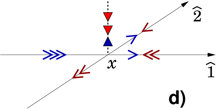
In Fig. 2 we show four examples of admissible flux-monomer net fluxes $f_{x}$ at a site $x$ . The first example (Fig. 2a) is a double line of flux entering from the negative 1-direction, which then splits at $x$ and two single fluxes exit in 1- and in 2-direction. The non-vanishing variables are $l_{x-\hat{1},1}=2,l_{x,1}=1,l_{x,2}=1$ . All other flux and monomer variables attached to $x$ vanish. The total net flux is $f_{x}=0$ . In Fig. 2b a double line of $l$ -flux enters and is compensated by two units of the monomer variable ( $l_{x-\hat{2},2}=2,s_{x}=2$ , $f_{x}=0$ ). Fig. 2c shows an example of a non-zero total flux $f_{x}=-6$ generated by a combination of nonvanishing $l$ - and $\overline{l}$ -fluxes, as well as monomers ( $l_{x-\hat{1},1}=1,l_{x-\hat{2},2}=1,\overline{l}_{x-\hat{2},2}=1,\overline{l}_{x,1}=2,\overline{l}_{x,2}=1,\overline{s}_{x}=2$ ). Finally Fig. 2d is an example with $f_{x}=-3$ , described by $l_{x-\hat{1},1}=3,\overline{l}_{x-\hat{2},2}=2,l_{x,1}=1,l_{x,2}=1,\overline{l}_{x,1}=2,\overline{l}_{x,2}=1,s_{x}=1,\overline{s}_{x}=2$ . The configurations in the sum $\sum_{\{l,\overline{l},s,\overline{s}\}}$ are then obtained by combining admissible flux arrangements at all sites $x$ .

The graphical representation will be useful for developing generalized Prokof’ev-Svistunov worm algorithms [11] which may be used to update the flux representation efficiently [13]. Furthermore, one can expand the partition sum (13) for small $\tau$ . Such a result will be important to check the outcome of numerical simulations (see also [6]), and the graphical representation is a highly welcome tool for organizing the terms of such an expansion.

Flux representation of observables

For a successful application of the flux representation of the effective theory in a Monte Carlo simulation also the observables have to be expressed in terms of flux and monomer variables. We here briefly discuss this issue for simple bulk and fluctuation observables. In particular we focus on the expectation value $\langle P\rangle$ of the Polyakov loop, where $P=\sum_{x}\mathrm{Tr}\,P(x)$ , the corresponding susceptibility $\chi_{P}=\langle P^{2}\rangle-\langle P\rangle^{2}$ , the internal energy $U=\langle S\rangle$ (where $S$ is the action (1)), and the heat capacity $C=\langle S^{2}\rangle-U^{2}$ . These quantities may be obtained as simple derivatives of the partition sum,

	$\displaystyle\langle P\rangle\;=\;\frac{1}{Z}\frac{\partial}{\partial\eta}\,Z\;,$		(17)
	$\displaystyle\chi_{P}\;=\;\frac{1}{Z}\frac{\partial^{2}}{\partial\eta^{2}}\,Z\,-\,\langle P\rangle^{2}\;,$
	$\displaystyle U\,=\,\frac{1}{Z}\,\bigg[\tau\frac{\partial}{\partial\tau}\,+\,\eta\frac{\partial}{\partial\eta}\,+\,\overline{\eta}\frac{\partial}{\partial\overline{\eta}}\bigg]\,Z\;,$
	$\displaystyle C=\frac{1}{Z}\bigg[\tau^{2}\frac{\partial^{2}}{\partial\tau^{2}}+\eta^{2}\frac{\partial}{\partial\eta^{2}}+\overline{\eta}^{2}\frac{\partial}{\partial\overline{\eta}^{2}}+2\tau\eta\frac{\partial^{2}}{\partial\tau\partial\eta}+2\tau\overline{\eta}\frac{\partial^{2}}{\partial\tau\partial\overline{\eta}}+2\eta\overline{\eta}\frac{\partial^{2}}{\partial\eta\partial\overline{\eta}}\bigg]Z-U^{2}.$

From the final form (13) of the partition sum it is obvious that the derivatives in (17) may be pulled under the sum over all flux and monomer configurations and there only act on the weight factor ${\cal W}[l,\overline{l},s,\overline{s}]$ , since the constraint is independent of $\tau,\eta$ and $\overline{\eta}$ . To perform the needed derivatives we write the weight factor as

{\cal W}[l,\overline{l},s,\overline{s}]\;=\;\tau^{L+\overline{L}}\;\eta^{S}\;\overline{\eta}^{\overline{S}}\;\left(\prod_{x,\nu}\;\frac{1}{l_{x,\nu}!\;\overline{l}_{x,\nu}!}\right)\left(\prod_{x}\;\frac{1}{s_{x}!\;\overline{s}_{x}!}\right)\,{\cal I}[l,\overline{l},s,\overline{s}]\;,

(18)

where we introduced abbreviations for the sums of flux and monomer variables

L\;=\;\sum_{x,\nu}l_{x,\nu}\;,\;\;\;\overline{L}\;=\;\sum_{x,\nu}\overline{l}_{x,\nu}\;,\;\;\;S\;=\;\sum_{x}s_{x}\;,\;\;\;\overline{S}\;=\;\sum_{x}\overline{s}_{x}\;.

(19)

Using the weight factor (18) one immediately obtaines the following relations:

\frac{\partial}{\partial\eta}{\cal W}[l,\overline{l},s,\overline{s}]\;=\;\frac{S}{\eta}\,{\cal W}[l,\overline{l},s,\overline{s}]\;,\;\;\;\frac{\partial^{2}}{\partial\eta^{2}}{\cal W}[l,\overline{l},s,\overline{s}]\;=\;\frac{S^{2}-S}{\eta^{2}}\,{\cal W}[l,\overline{l},s,\overline{s}]\;,

(20)

for the derivatives with respect to $\eta$ , and similar relations for the derivatives with respect to the other parameters. The important aspect of the expressions (20) is that the derivatives of the weight factor may be written as the unchanged weight ${\cal W}[l,\overline{l},s,\overline{s}]$ , multiplied with factors built from the parameters $\eta,\overline{\eta},\tau$ and the sums (19) of flux- and monomer variables. Reinserting these relations we obtain rather simple expressions for our observables (17),

	$\displaystyle\langle P\rangle\;=\;\frac{1}{\eta}\langle S\rangle\;,$		(21)
	$\displaystyle\chi_{P}\;=\;\frac{1}{\eta^{2}}\,\Big[\,\langle S^{2}-S\rangle\;-\;\langle S\rangle^{2}\,\Big]\;,$
	$\displaystyle U\;=\;\langle\,L+\overline{L}+S+\overline{S}\,\rangle\;,$
	$\displaystyle C\;=\;\langle\,(\,L+\overline{L}+S+\overline{S}\,)^{2}\,\rangle\,-\,U\,-\,U^{2}\;.$

Obviously all the bulk and fluctuation observables we list here can be expressed in terms of the (summed) flux and monomer occupation numbers from Eq. (19), as well as the corresponding fluctuations.

As a matter of fact, in a similar way also correlators can be expressed in terms of the flux and monomer variables. We briefly discuss this for the example of the Polyakov loop correlator $\langle\,\mathrm{Tr}P(x)\,\mathrm{Tr}P(y)^{\dagger}\,\rangle$ . The two factors $\mathrm{Tr}P(x)$ and $\mathrm{Tr}P(y)^{\dagger}$ can be generated from the partition sum by using parameters $\eta(x)$ and $\overline{\eta}(x)$ in (1), which are independent parameters for all sites $x$ of the lattice. The mapping of this generalized model with locally varying parameters to the flux-monomer representation goes through unchanged. The local parameters $\eta(x)$ and $\overline{\eta}(x)$ can now be used as sources and the correlator $\langle\,\mathrm{Tr}P(x)\,\mathrm{Tr}P(y)^{\dagger}\,\rangle$ is obtained via two partial derivatives. In the end one sets all parameters to the original values, i.e., $\eta(x)=\eta$ and $\overline{\eta}(x)=\overline{\eta}$ for all $x$ . One ends up with

\langle\,\mathrm{Tr}P(x)\,\mathrm{Tr}P(y)^{\dagger}\,\rangle\;=\;\frac{1}{Z}\,\frac{\partial^{2}}{\partial\eta(x)\,\partial\overline{\eta}(y)}\,Z\;\Bigg|_{{\eta(x)=\eta\atop\overline{\eta}(x)=\overline{\eta}}}\;=\;\;\frac{1}{\eta\,\overline{\eta}}\,\langle\,s_{x}\,\overline{s}_{y}\,\rangle\;.

(22)

We find that the Polyakov loop correlator turns into a correlator of the monomer numbers at the corresponding sites. In a simulation of the flux-monomer representation with a worm algorithm one can evaluate this correlator by directly sampling the starting point of the worm correlated with its actual position and with this improved estimator one expects to get an excellent signal.

Summary, discussion, outlook

In this article we study an effective Polyakov loop theory for QCD thermodynamics. The model may be obtained from a strong coupling expansion, combined with a hopping expansion for the fermion determinant. It contains the leading center symmetric and center symmetry breaking terms. At non-zero chemical potential the model inherits the complex phase problem of finite density QCD. The complex phase problem prohibits a direct Monte Carlo simulation in the standard representation.

Using high temperature expansion techniques, we map the partition sum of the effective Polyakov loop model to a representation where the dynamical degrees of freedom are integer valued flux variables attached to the links of the lattice, and integer valued monomer variables at the sites. The flux-monomer configurations are subject to a constraint which forces the local net flux at each site to have vanishing triality, i.e., the flux has to be a multiple of three. All admissible configurations come with a real and positive weight factor, and thus in the flux-monomer representation the complex phase problem is solved.

For systems with such a flux representation generalizations of the Prokof’ev-Svistunov worm algorithm [11] allow for a numerical Monte Carlo simulation of the model. As a matter of fact, for a similar QCD-related system a generalized worm algorithm was used to effectively explore the full temperature and chemical potential parameter space, also in regions where the complex phase problem is severe [6]. We expect [13] that for the system discussed here, a worm algorithm with similar efficiency can be implemented on the basis of the new flux-monomer representation given here. Again it should be possible to explore the full temperature-density phase diagram. Such an analysis will provide interesting insight into various aspects of the phase structure of QCD-related systems.

Besides the improvement of our physical understanding, a simulation based on the new flux representation will also have important technical applications. The models can serve as a prototype system, which other approaches to QCD with non-zero chemical potential can be tested against. Various expansions in $\mu$ , imaginary chemical potential techniques, as well as results from reweighting (see [14] for reviews) could be compared to the outcome of a Monte Carlo simulation in the flux representation, where the simulation is not tainted by uncontrolled effects from a complex phase problem.

However, not only lattice techniques should be compared to the prototype system presented here. It is straightforward to write down a continuum counterpart of the action (1), and the system could also be analyzed with various continuum techniques, in particular functional methods [15]. A comparison of these results with the lattice would provide important insights on the assumptions and the reliability of the continuum techniques.

Acknowledgments

The author thanks Gert Aarts, Ydalia Delgado-Mercado, Hans Gerd Evertz, Christian Lang, Bernd-Jochen Schaefer, Owe Philipsen and Andreas Wipf for stimulating discussions and remarks on the literature.

References

[1] L.G. Yaffe and B. Svetitsky, Phys. Rev. D 26 (1982) 963; Nucl. Phys. B 210 423. A.M. Polyakov, Phys. Lett. B 72 (1978) 477. L. Susskind, Phys. Rev. D 20 (1979) 2610.
[2] A. Patel, Nucl. Phys. B 243 (1984) 411; Phys. Lett. B 139 (1984) 394. T. DeGrand and C. DeTar, Nucl. Phys. B 225 (1983) 590. J. Condella and C. DeTar, Phys. Rev. D 61 (2000) 074023 [arXiv:hep-lat/9910028].
[3] J. Polonyi, K. Szlachanyi, Phys. Lett. B110 (1982) 395-398. F. Green, F. Karsch, Nucl. Phys. B238 (1984) 297. A. Gocksch, M. Ogilvie, Phys. Rev. D31 (1985) 877.
[4] R.V. Gavai, F. Karsch and B. Petersson, Nucl. Phys. B 322 (1989) 738. F. Karsch and S. Stickan, Phys. Lett. B 488 (2000) 319 [arXiv:hep-lat/0007019].
[5] M.G. Alford, S. Chandrasekharan, J. Cox and U.-J. Wiese, Nucl. Phys. B 602 (2001) 61 [arXiv:hep-lat/0101012]. S. Kim, P. de Forcrand, S. Kratochvila and T. Takaishi, PoS LAT2005 (2006) 166 [arXiv:hep-lat/0510069]. P. de Forcrand, O. Philipsen, Phys. Rev. Lett. 105 (2010) 152001 [arXiv:1004.3144 [hep-lat]].
[6] Y. D. Mercado, H. G. Evertz, C. Gattringer, [arXiv:1102.3096 [hep-lat]].
[7] L. Dittmann, T. Heinzl, A. Wipf, JHEP 0406 (2004) 005 [hep-lat/0306032]. C. Wozar, T. Kaestner, A. Wipf, T. Heinzl, B. Pozsgay, Phys. Rev. D74 (2006) 114501 [hep-lat/0605012]. C. Wozar, T. Kaestner, A. Wipf, T. Heinzl, Phys. Rev. D76 (2007) 085004 [arXiv:0704.2570 [hep-lat]]. A. Wipf, T. Kaestner, C. Wozar, T. Heinzl, SIGMA 3 (2007) 006 [hep-lat/0610043]. C. Wozar, T. Kastner, B. H. Wellegehausen, A. Wipf, T. Heinzl, PoS LATTICE2008 (2008) 257 [arXiv:0808.4046 [hep-lat]]. C. Wozar, T. Kaestner, S. Uhlmann, A. Wipf, T. Heinzl, PoS LAT2007 (2007) 341 [arXiv:0708.4146].
[8] J. Langelage, S. Lottini, O. Philipsen, JHEP 1102 (2011) 057 [arXiv:1010.0951 [hep-lat]]. J. Langelage, S. Lottini, O. Philipsen, PoS LATTICE2010 (2010) 196 [arXiv:1011.0095 [hep-lat]]. J. Langelage, O. Philipsen, JHEP 1001 (2010) 089 [arXiv:0911.2577 [hep-lat]]. J. Langelage, G. Münster, O. Philipsen, JHEP 0807 (2008) 036 [arXiv:0805.1163 [hep-lat]].
[9] T. Z. Nakano, K. Miura, A. Ohnishi, Prog. Theor. Phys. 123 (2010) 825 [arXiv:0911.3453 [hep-lat]]; PoS LATTICE2010 (2010) 205 [arXiv:1010.5687 [hep-lat]].
[10] F. Karsch and H.W. Wyld, Phys. Rev. Lett. 55 (1985) 2242. N. Bilic, H. Gausterer, S. Sanielevici, Phys. Rev. D 37 (1988) 3684.
[11] N. Prokof’ev and B. Svistunov, Phys. Rev. Lett. 87 (2001) 160601.
[12] S. Uhlmann, R. Meinel, A. Wipf, J. Phys. A A40 (2007) 4367-4390 [hep-th/0611170].
[13] Work in preparation.
[14] P. de Forcrand, PoS LAT2009 (2009) 010 [arXiv:1005.0539 [hep-lat]]. S. Gupta, PoS LATTICE2010 (2010) 007. [arXiv:1101.0109 [hep-lat]].
[15] P. Kopietz, L. Bartosch, F. Schutz, Lect. Notes Phys. 798 (2010) 1-380.

Abstract

We discuss an effective Polyakov loop model for QCD thermodynamics with a chemical potential. Using high temperature expansion techniques the partition sum is mapped exactly onto the partition sum of a flux model. In the flux representation the complex action problem is resolved and a simulation with worm-type algorithms becomes possible also at finite chemical potential.