Hierarchies of Susy Splittings in Holographic Gauge Mediation
Abstract:
We generalize to string theory a construction, originally proposed in field theory, that generates a hierarchy in the splittings between members of super-multiplets in various sectors of the theory.
Keywords:
Gauge mediation, superpartner splitting, gauge/gravity duality1 Introduction
In a previous paper [1], we explored how to generate hierarchies in the splittings between superpartners in gauge mediation scenarios ([2] to [7]). We considered the cases in which the hierarchy is such that there is an “almost supersymmetric” sector that is largely decoupled from the visible sector. The discussion in that paper was in a field theoretical context and, from that construction, it was possible to identify candidates for “invisible” dark matter in addition to the generation of a very flat scalar potential for the inflaton field.
In this paper we extend the study of those hierarchies to the string theory context. More specifically, we explore the generation of hierarchies in the SUSY-breaking mass contributions for different sectors using the holographic gauge mediation proposed in [8] with the techniques the Klebanov-Strassler gauge/gravity duality [11]. In that work, a metastable non-supersymmetric construction is used in a deformed conifold embedding [15]. The matter field content is realized by introducing a set of D7-branes. Here, we will analyze the possibilities of introducing additional matter sectors by using two separate stacks of D7-branes. These two sets of D7s can be thought of as the result of splitting an original stack (with a small number of D-branes, for instance, 7). As a result, we obtain a set of sectors with different mass splittings like those in [1], although there are some extra features that were not present in the original work [1]; for example, some massive vector mesons that weakly connect the visible and invisible sectors.
This article is organized as follows: The first section is dedicated to a quick review of the deformed conifold and the metastable non-supersymmetric system. In the second section, we describe the construction of hierarchies in the splitting in the holographic scenario. We close with some conclusions.
2 The deformed conifold and SUSY breaking
The work in [8] realized gauge mediation of supersymmetry breaking by using the deformed conifold geometry. The warped deformed conifold [11] is a solution of type IIB SUGRA on (where is the base of the conifold), which is dual to the IR limit of the supersymmetric field theory arising from a set of D3-branes and wrapped D5-branes in the strong ‘t Hooft coupling limit. The gauge group for this theory is and the superpotential for the bifundamental fields, and , is given by [9]
| (1) |
The singular conifold is parametrized by the holomorphic equation
| (2) |
The metric for the background may be written as
| (3) |
where
| (4) |
The warp factor is obtained from the solution to the trace of the Einstein’s equation. The result is
| (5) |
where is the UV scale. This was presented by Klebanov and Tseytlin (KT) in [10]. This solution has a naked singularity at some for which .
In the solution to the SUGRA equations, the 5-form flux acquires a radial logarithmic dependence,
| (6) |
where
| (7) |
and
| (8) |
The forms and are defined in equation (44) in the appendix.
As the flux goes through a period, will decrease units, which decreases the 5-form by units as well. This behavior is matched to the cascade of Seiberg dualities [12] that occur in the dual gauge theory. One consequence is that, as the theory flows to the IR, the cascade must stop since cannot be negative. In gravity/gauge duality, the radial coordinate defines the RG scale of the dual theory: [13]. The two gauge couplings are determined by
| (9) |
| (10) |
for a vanishing dilaton field.
When becomes small, Klebanov and Strassler argued that the above solution (KT) must be modified in order to remove the singularity. Thus, the conifold is replaced by the deformed conifold
| (11) |
Indeed, they showed that, in the infrared, the field theory is strongly coupled and has a deformed moduli space, which has independent branches and each has the geometry of a deformed conifold.
For the case , when a set of anti-D3-branes are added to the above configuration, the system has a metastable non-SUSY vacuum [14]. At the end of the duality cascade (after steps), there are only the fractional D3-branes and the anti-D3-branes left. The anti-D3-branes experience a potential towards the bottom of the throat but they are not allowed to reach the origin since the conifold has now a tip; thus, they reach a metastable vacuum. At some point, this state will decay to a supersymmetric vacuum. This occurs when the surrounding flux induces them to puff up to a NS5-brane wrapping the on the tip. The NS5-brane is a source for the flux and, as the brane moves to the minimum in the brane/flux potential, it changes the flux by -1 units. This results in a supersymmetric theory with D3-branes. The metastable state is parametrized by the vacuum energy
| (12) |
DeWolfe, Kachru and Mulligan (DKM) [15] found a solution (to first order) for the backreaction of anti-D3-branes in the KT solution, which is the asymptotic UV approximation of the KS solution. In this case, the metric is
| (13) |
where , and are 1-forms that are defined in equation (43).
The SUGRA solution in the Einstein frame, as written in the appendix of [8], is:
| (14) |
| (15) | |||||
| (16) | |||||
| (17) | |||||
| (18) |
where the last four equations include the first corrections in and .
3 Holographic gauge mediation and splitting hierarchies
Following the procedure described in [8] for one matter sector, we will use the warped deformed conifold geometry from the previous section to realize gauge mediation to two separate sectors. The first sector (which we will call “visible”) is a stack of D7-branes () which are holomorphically embedded according to Kuperstein construction [17] 11 1 There are other possible embeddings of D7s in the KS geometry; see, for example, [18]. :
| (19) |
These D7s fill the four space-time dimensions, extend along the radial coordinate of the conifold and wrap a three-cycle of . The matter fields of this sector (the standard model) are placed at the UV cutoff of the geometry, which implies that the SM fields, on the gauge side, are elementary fields and are decoupled from the hidden sector strong interactions.
Likewise, the second sector (“invisible”) is a set of D7-branes ( placed farther than the first stack from the tip of the conifold (see figure 1):
| (20) |
As for the “visible” sector, the “invisible” sector can also have a matter content at the UV end of the geometry, from which we can obtain a set of elementary particles that are not coupled to the standard model particles.

This theory contains two sets of chiral fields arising from the D7-D3 strings. We have and which transform as and , respectively. Here, the first element is one of the conifold gauge groups and the second one is the “visible” sector gauge group. Similarly, we have a second set of chiral fields, and , which transform as and , under the conifold gauge group and the gauge group of the second sector (“invisible” sector). These fields are the messengers of the supersymmetry breaking. The tree-level superpotential is written as
| (21) | |||||
The two types of fields, and , have dimension and masses and , respectively.
We now turn to study the gauge mediation of the SUSY breaking to each of the sectors. There are, in fact, two regimes in which one can compute the soft mass for the gaugino. The first case is when the mass of the messengers is of the same order as the confining scale of the hidden sector, i.e. . Thus, the D7s are close to the anti-D3s and we need to use the SUGRA solution close to the tip of the conifold in order to compute the gaugino mass. This approach was studied in [16] and we will not use it here.
The second regime is the one in which . This is the scenario proposed in [8] and the one we will use in the rest of this paper. In this case, calculations can be made at large radius on the gravity side (using the KT limit of the KS geometry). Since the messengers are strongly coupled under the conifold gauge group, they form mesons (or ) which transform in the adjoint representation of the visible (or invisible) gauge group and are weakly coupled.
The masses and -terms for those mesons are computed using holography, where the DBI action for the D7s is dimensional reduced and, as a result, the Kaluza-Klein modes (which are fluctuactions of equations (19) and (20)) adquire both supersymmetric and soft masses. The loop interactions of these mesons with the visible (invisible) sector will generate mases for the corresponding gaugino, since -symmetry is broken by the non-zero -term. This sort of gauge mediation, in which the messengers do not participate in the supersymetry breaking, is closely related to “semi-direct gauge mediation” [19]. In addition, there are some strings that connect both stacks of D7s. Since we are assuming a large hierarchy between and , the states resulting from these strings are quite heavy and the contributions to the masses in either sector are very suppressed.
The bosonic action for the mesons that is obtained from the expansion of the DBI action to quadratic order has the form 22 2 This is a simplified expression that allows us to describe the general form of the soft mass contribution from the mesons. For specific details of the calculation, see the appendices of [8].
| (22) | |||||
| (23) | |||||
| (24) | |||||
where refers to the stack of D7-branes at and are the small fluctuations about . Likewise, corresponds to the second set of D7s. and are the respective induced metrics on the D-branes and are the metrics of the DKM geometry as defined in equation (48) in the appendix. Here, .
The next step is to expand and in Kaluza-Klein modes,
| (25) |
where denotes the internal coordinates of the D7-brane and denotes the four-dimensional space-time. After plugging these expansions into equations (23, 24), we obtain the scalar potential
| (26) |
where
| (27) | |||||
| (28) |
| (29) | |||||
| (30) |
This corresponds, in the superfield formalism, to a superpotential
| (31) |
where
and
After introducing the expressions from the DKM metric and integrating over the extra-dimensions, one finds, as in [8],
| (32) | |||
| (33) |
In the last equations,
Thus, we notice that the hierarchy between the mass of the messenger mesons is given by
| (34) |
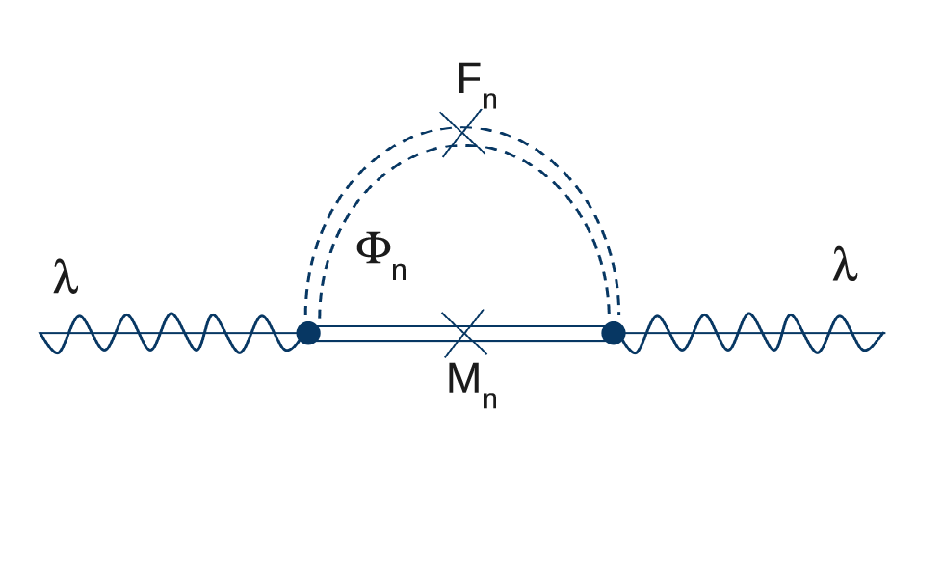
The gaugino masses for each of the sectors can be computed using field theory. The 1-loop contribution (figure 2) gives
| (35) |
and
| (36) |
where are phases coming from the fact that the -terms are complex. The sum over is constrained by the binding energy of the mesons, or , which implies . A lower bound for is given by the validity of the DBI expansion:
| (37) |
The authors of [8] noticed that there is a second contribution, due to the deformation in the KS geometry, given by
| (38) |
which is much smaller than the contributions from the loop considered above.
An important remark is that, in order to avoid a Landau pole for the visible and invisible gauge couplings, the geometry must have a cutoff, which implies a constraint for the number of steps in the duality cascade: . The authors of [8] suggested that this constraint might be avoided by working with orbifold geometries.
On the phenomenology aspect of this construction, taking and and , we can recreate similar parameters to those in [1]. For that purpose, we obtain that
| (39) |
gives a visible gaugino mass of the order of the electroweak scale. For the invisible sector, if we consider
| (40) |
we get light “dark” gauginos () which may be interesting candidates for “invisible” components of dark matter. In this context, one could also break the gauge symmetry in the invisible sector by separating the two D7-branes which would imply the emergence of invisible massive vector bosons and monopoles.
4 Conclusions
We did exhibit in this paper a way to generate hierarchies in the soft masses, for different matter sectors. This was achieved in string theory using gauge/gravity duality. More specifically, we used a warped deformed conifold background with a holomorphic embedding of D7-branes. The hierarchy between the radial position of the two stacks of D7s determined the hierarchy between the messenger masses and, hence, the hierarchy in the SUSY breaking splittings. This kind of hierarchies has phenomenological implications for cosmological models which were studied in previous papers [1, 20]. It remains important to achieve in string theory, in the context of the construction presented here, a cosmology consistent with observations.
5 Acknowledgments
The research of W.F. and W. T. G. was supported in part by the National Science Foundation under Grant Numbers PHY-0969020 and PHY-0455649. W. T. G. would like to thank Elena Cáceres for helpful conversations and the Texas Cosmology Center for partial support.
Appendix A Some definitions on the conifold geometry
A.1 The singular conifold
The unwarped metric on the conifold is given by
| (41) |
| (42) | |||||
where
| (43) |
For more information on the geometric structure of the conifold, see [21].
A.2 Kuperstein embedding in the DKM solution
A holomorphic embedding of a set of D7-branes is given by Kuperstein [17]
| (45) |
The work in [8] used the following parametrization of the holomorphic coordinates of the conifold, where are functions of a new set of coordinates :
| (46) |
with , , , , , and , are the transverse coordinates.
With this parametrization,
| (47) |
ant the DKM metric is written as
| (48) |
where the forms are defined as
| (49) |
The 2-form is written as
| (50) |
References
- [1] W. Fischler and W. Tangarife Garcia, Hierarchies of SUSY splittings and invisible photinos as dark matter, JHEP 1101 025 (2011), [arXiv:1011.0099].
- [2] M. Dine, W. Fischler, M. Srednicki, Supersymmetric Technicolor, Nucl. Phys. B 189,575 (1981).
- [3] S. Dimopoulos and S. Raby, Supercolor, Nucl. Phys. B 192, 353 (1981).
- [4] C . R. Nappi and B. A. Ovrut, Supersymmetric Extension Of The Model, Phys. Lett. B 113, 175 (1982).
- [5] L. Alvarez-Gaume, M. Claudson and M. B. Wise, Low-Energy Supersymmetry, Nucl. Phys. B 207, 96 (1982).
- [6] M. Dine and W. Fischler, A Phenomenological Model Of Particle Physics Based On Supersymmetry, Phys. Lett. B 110, 227 (1982).
- [7] M. Dine and W. Fischler, A Supersymmetric GUT, Nucl. Phys. B 204, 346 (1982).
- [8] F. Benini, A. Dymarski, S. Franco, S. Kachru, D. Simic and H. Verlinde, Holographic Gauge Mediation, JHEP 0912, 031 (2009), [arXiv:0903.0619].
- [9] I. R. Klebanov, E. Witten, Superconformal field theory on three-branes at a Calabi-Yau singularity, Nucl. Phys. B536, 199-218 (1998). [arXiv:hep-th/9807080].
- [10] I. R. Klebanov and A. Tseytlin, Gravity duals of supersymmetric gauge theories, Nucl. Phys. B578 (2000) 123, [arXiv:hep-th/0002159].
- [11] I. R. Klebanov and M. J. Strassler, Supergravity and a confining gauge theory: Duality cascades and SB resolution of naked singularities, JHEP 0008, 052 (2000), [arXiv:hep-th/0007191].
- [12] N. Seiberg, Electric - magnetic duality in supersymmetric nonAbelian gauge theories, Nucl. Phys. B435, 129-146 (1995). [hep-th/9411149].
- [13] J. M. Maldacena, The Large N limit of superconformal field theories and supergravity, Adv. Theor. Math. Phys. 2, 231 (1998) [Int. J. Theor. Phys. 38, 1113 (1999)] [arXiv:hep-th/9711200].
- [14] S. Kachru, J. Pearson and H. Verlinde, Brane/flux annihilation and the string dual of a non-supersymmetric field theory, JHEP 0206, 021 (2002), [arXiv:hep-th/0112197].
- [15] O. DeWolfe, S. Kachru and M. Mulligan, A gravity dual of metastable dynamical supersymmetry breaking, Phys. Rev. D 77, 065011 (2008). [arXiv:0801.1520].
- [16] P. Mcguirk, G. Shiu and Y. Sumitomo, Holographic gauge mediation via strongly coupled messengers, Phys. Rev. D 81, 026005 (2010), [arXiv:0911.0019].
- [17] S. Kuperstein, Meson spectroscopy from holographic probes on the warped deformed conifold, JHEP 0503, 014 (2005), [arXiv:hep-th/0411097].
- [18] P. Ouyang, Holomorphic D7 branes and flavored N=1 gauge theories, Nucl. Phys. B699, 207-225 (2004). [hep-th/0311084].
- [19] N. Seiberg, T, Volansky and B. Wecht, Semi-direct gauge mediation, JHEP 0811, 004 (2008), [arXiv:0809.4437].
- [20] W. Fischler and J. Meyers, Dark Radiation Emerging After Big Bang Nucleosynthesis?, Phys. Rev. D 83, 063520 (2011) [arXiv:1011.3501].
- [21] P. Candelas, X. de la Ossa, Comments on conifolds, Nucl. Phys. B 342, 246 (1990).