The effects of strong temperature anisotropy on the kinetic structure of collisionless slow shocks and reconnection exhausts. Part II: Theory
Abstract
Simulations of collisionless oblique propagating slow shocks have revealed the existence of a transition associated with a critical temperature anisotropy = 0.25 (Liu, Drake and Swisdak (2011)[1]). An explanation for this phenomenon is proposed here based on anisotropic fluid theory, in particular the Anisotropic Derivative Nonlinear-Schrödinger-Burgers equation, with an intuitive model of the energy closure for the downstream counter-streaming ions. The anisotropy value of 0.25 is significant because it is closely related to the degeneracy point of the slow and intermediate modes, and corresponds to the lower bound of the coplanar to non-coplanar transition that occurs inside a compound slow shock (SS)/rotational discontinuity (RD) wave. This work implies that it is a pair of compound SS/RD waves that bound the outflows in magnetic reconnection, instead of a pair of switch-off slow shocks as in Petschek’s model. This fact might explain the rareness of in-situ observations of Petschek-reconnection-associated switch-off slow shocks.
I Introduction
Shocks in isotropic MHD have been intensively studied, including the existence of intermediate shocks (IS) ([2, 3, 4, 5] and references therein), the occurrence of dispersive wavetrains [6, 7, 8], and the nested subshocks inside shocks predicted by the Rankine-Hugoniot jump conditions [9, 10]. In a collisionless plasma, the effects of temperature anisotropy need to be considered, which can be done for linear waves with the Chew-Goldberger-Low (CGL) framework [11, 12]. Hau and Sonnerup have pointed out the abnormal properties of the linear slow mode under the influence of a firehose-sense () pressure anisotropy, including a faster phase speed compared to the intermediate mode, a fast-mode-like positive correlation between magnetic field and density, and the steepening of the slow expansion wave. In kinetic theory both anisotropy and high can greatly alter the linear mode behavior [13, 14]. The anisotropic Rankine-Hugoniot jump conditions have been explored while taking the downstream anisotropy as a free parameter [15, 16, 17, 18], while Hudson [17] calculated the possible anisotropy jumps across an anisotropic rotational discontinuity. Karimabadi et al. [14] noticed the existence of a slow shock whose upstream and downstream are both super-intermediate. But, a comprehensive nonlinear theory describing the coupling between slow and intermediate shocks under the influence of temperature anisotropy has not yet been presented.
In Petschek’s description of magnetic reconnection, the reconnection exhaust is bounded by a pair of back-to-back standing switch-off slow shocks. Particle-in-cell (PIC) simulations of such shocks [1, 19] exhibit large downstream temperature anisotropies. In Liu et al. (2011) [1] (hereafter called Paper I) and Fig. 1 of this paper we show that when the parameter , the behavior of the coplanar shock undergoes a transition to non-coplanar rotation. This firehose-sense temperature anisotropy slows the linear intermediate mode and speeds up the linear slow mode enough so that, at some point, their relative velocities can be reversed [11, 12]. This reversal is reflected in the structure of the Sagdeev potential (also called the pseudo-potential) [20], which characterizes the nonlinearity of the system. In this work a simplified theoretical model is developed to explore the effect of temperature anisotropy on the structure of the Sagdeev potential and to provide an explanation for the extra transition inside the switch-off slow shock (SSS) predicted by isotropic MHD. The theory suggests that in PIC simulations a compound slow shock (SS)/ rotational discontinuity (RD) is formed instead of a switch-off slow shock. This work may help to explain satellite observations of compound SS/RD waves [21, 22], anomalous slow shocks [23] and the trapping of an RD by the internal temperature anisotropy of a slow shock in hybrid simulations [24].
In Sec. II of this paper we introduce our model equations for studying the nonlinear coupling of slow and intermediate waves under the influence of a temperature anisotropy. In Sec. III we calculate the speeds and the eigenmodes of slow and intermediate waves. Sec. IV points out the existence of extra degeneracy points between slow and intermediate modes introduced by the temperature anisotropy, and comments on the consequences (in the context of the Riemann problem) of having the slow wave faster than the intermediate wave. In Sec. V we introduce a simple energy closure. In Sec. VI. A. we calculate the pseudo-potential of stationary solutions, and apply the equal-area rule to identify the existence of compound SS/RD waves and compound SS/IS waves. In Sec. VI. B we demonstrate the significance of as being the lower bound of the SS to RD transition in compound SS/RD waves. In Sec. VII we discuss the time-dependent dynamics that help keep . In Sec VIII we provide more evidence from PIC simulations to support the existence of compound SS/RD waves at the boundaries of reconnection exhausts. In Sec IX, we summarize the results and point out the relation between compound SS/RD waves and anisotropic rotational discontinuities [17].
II The Anisotropic Derivative Nonlinear Schrödinger-Burgers equation
Instead of analyzing the anisotropic MHD equations, which have seven characteristics (waves), we simplify the system into a model equation that possesses only two characteristics. This model equation will be ideal for demonstrating the underlying coupling between the nonlinear slow and intermediate modes. Beginning with the anisotropic MHD equations [15], we follow the procedure of Kennel et al. [4, 25] to derive the Anisotropic Derivative Nonlinear Schrödinger-Burgers equation (ADNLSB) (see Appendix I for details),
| (1) |
This equation describes waves that propagate in the -direction in the upstream intermediate speed frame. In this frame is the spatial coordinate with , and is the time used to measure the slow variations (such as steepening processes). , where the subscript “” represents the component tangential to the wave-vector and here will be in the - plane. The anisotropy parameter . The subscript “0” denotes the upstream parameters. The right hand side term proportional to the ion inertial length, , represents dispersion (which can be viewed as the spreading tendency of Fourier decomposed waves of different wavenumbers), while the term containing describes dissipation from magnetic resistivity. Here is a constant. The terms proportional to and are the nonlinearities of this wave equation, where
| (2) |
| (3) |
and
| (4) |
Here and for monatomic plasma. Since we are studying reconnection exhausts, (the angle between the upstream magnetic field and ) is typically large (). Therefore , and . Hence this equation describes only the slow and intermediate modes [4] (this is shown explicitly in the next section). This fact relates to the degeneracy properties of ideal MHD for parallel propagating waves, namely that the fast and intermediate modes degenerate in plasmas, while the slow and intermediate mode degenerate in plasmas. Finally, we note that Eq. (1) is applicable in the weak nonlinearity limit.
III The conservative form- wave propagation
In order to explore the structure of the reconnection exhaust, a comprehensive understanding of how waves connect to each other across a transition is required. This is called a Riemann problem. Neglecting the source terms on the right hand side (RHS), the left hand side (LHS) of Eq. (1) is a hyperbolic equation in conservative form.
Letting , and , we obtain,
| (5) |
with
We can obtain the characteristics (waves) of this equation by analyzing its flux function, f. Its Jacobian is
| (14) |
where , . One eigenvalue (also called the characteristic speed) is
| (15) |
with eigenvector
| (16) |
In isotropic ideal MHD, where the term is dropped, the eigenvalue in the infinitesimal limit () is , which is the phase speed of the linear slow mode in the intermediate mode frame. The subscript “SL” means the slow mode. The eigenvector indicates that slow mode is coplanar (i.e., in the radial direction in space).
The other mode has eigenvalue
| (17) |
and eigenvector
| (18) |
In isotropic ideal MHD, where the term is dropped, the eigenvalue in the infinitesimal limit is , which is the phase speed of the linear intermediate mode in the intermediate mode frame. The subscript “I” means the intermediate mode. The eigenvector indicates that this intermediate mode is non-coplanar (i.e., in a non-radial direction).
It can be shown that for all . This means that along the eigen-direction of the intermediate mode the characteristic speed is constant, and thus the mode exhibits no steepening or spreading, just as is the case for its counterpart in isotropic MHD. (This behavior is also confirmed by the anisotropic MHD simple wave calculation; see Appendix II). Therefore the intermediate mode is termed “linearly degenerate”. If we are looking for a transition in the direction (toward , then the portion of the slow mode with will steepen into a slow shock. When at the downstream of a transition is larger than that at the upstream, the downstream wave will catch up with the upstream wave and thus steepen.
IV A new degeneracy point due to the temperature anisotropy
In the Riemann problem for our two mode system, we seek to determine the middle state that connects the faster “2-wave” from a given state , to the slower “1-wave” from a given state (see Fig. 2 (a); the subscripts “r” and “l” mean right and left respectively). In order to determine the path that connects to in the state space ( space, in this case), the Hugoniot locus that connects or to a possible asymptotic state by shock waves needs to be calculated, as do the integral curves for possible rarefaction waves (see, for example, [26]). The Hugoniot locus in state space is a curve formed by allowing one of the parameters in the standard Rankine-Hugoniot jump condition to vary. The integral curve is formed by following the eigenvector from a given state in state space.
In order to proceed we further assume a gyrotropic energy closure, , which allows us to write
The Hugoniot locus and integral curves of the intermediate mode are identical in our system. This is also the case for the slow mode (we perform the calculation in Appendix III). For a given state, , the Hugoniot locus and integral curve of the intermediate mode are
| (23) |
which is a circle in state space. Note that even though we can calculate the Hugoniot locus and integral curve for the intermediate mode, the solution is the same as for a finite amplitude intermediate mode that does not steepen into a shock or spread into a rarefaction. For the slow mode, the Hugoniot locus and integral curve are
| (24) |
which is in the radial direction in state space. This direction implies that the slow shock is coplanar, even in the presence of temperature anisotropy, just as is the case for its counterpart in full anisotropic MHD [15]. In the isotropic case, this curve forms a slow shock if the path is toward the origin, and a slow rarefaction if the path is away from the origin.
The state can connect to by following the Hugoniot locus of a slow mode that starts from , as shown in Fig. 2(b). In isotropic MHD this forms a switch-off slow shock. However, a strong enough temperature anisotropy introduces new degeneracy points (which occur where ) when , other than the traditional degeneracy point at . These points form a band circling the origin as shown in Fig. 2(c). Inside the band, the intermediate mode is slower than the slow mode. Physically, this implies that a rotational intermediate mode can arise downstream of a slow mode, something which is not allowed in a Riemann problem in isotropic MHD. This effect is realized when the path along the Hugoniot locus ( direction) of the slow mode from switches to the solution of the intermediate mode (circular direction) somewhere () inside the degeneracy band.
This behavior can explain the morphological differences between the shock simulations in the cases and those for of Paper I [1]. The latter has an extra transition to the rotational direction that is similar to the path in Fig. 2(c). We now look for a similar effect in state space and a way of determining in a more detailed analytical model.
V An energy closure based on counter-streaming ions
In order to close the ADNLSB equations, we need a energy closure . The modeling of the energy closure for a collisionless plasma has historically been difficult. The Chew-Goldberger-Low (CGL) condition [27] is one choice, but it does not work well when streaming ions are present. Since we are here just trying to qualitatively demonstrate the underlying physics, we will assume that we have a , where and are simply related by
| (25) |
with positive constants and and the condition is imposed. This functional form is motivated by the nearly constant parallel pressure maintained by free-streaming ions (). Although Eq. (25) is strictly empirical, results from PIC simulations (see Fig. 3) suggest that provides a reasonable first approximation and will be used in the following calculations.
We take the variation,
| (26) |
where . This parameterization will be valid whenever . Therefore, an effective nonlinearity in Eq. (1) can be written as,
| (27) |
The most important conclusions in the remainder of this work do not depend on the details of the closure, but only that decreases as decreases. Note that is mostly positive in the limit in which we are interested. This fact will be used in the following section.
VI The pseudo-potential: Looking for a stationary solution
VI.1 The formation of compound SS/RD waves and SS/IS waves
In order to determine both where the path in the state space of Fig. 2(c) will turn to the intermediate rotation and the nontrivial coupling of the slow and intermediate modes when temperature anisotropies are present, we construct the pseudo-potential of a stationary solution. We will look for a equation that possesses traveling stationary waves, by substituting (where is the speed of the stationary wave observed in the upstream intermediate frame) into Eq. (1) and integrating over once. We obtain
| (28) |
In this formulation we can treat as a spatial coordinate, and as time. The terms on the LHS of Eq. (28) behave analogously to, respectively, a frictional force and a Coriolis force with rotational frequency and rotational axis . A pseudo-potential that characterizes the nonlinearity is uniquely defined because . We are only interested in the small limit, because the upstream values with subscript “0” are expected to be the upstream values of a switch-off slow shock in ideal isotropic MHD, which propagates at the upstream intermediate speed. The anisotropy in our PIC simulations does not seem to significantly change this behavior [1].
Calculating the pseudo-work done on the pseudo-particle, , we obtain
| (29) |
Note that from upstream to downstream is in the negative direction. The pseudo-particle will move to a lower potential, while its total energy is dissipated by the resistivity and the rate of the drop depends on the strength of the resistivity. Kennel et al. [4] have shown that when pseudo-particles move toward lower pseudo-potentials, the entropy increases and so the resulting shock is admissible. Note that the Coriolis-like force does not do work. It only drives rotation of the pseudo-particle on the iso-surface of the pseudo-potential and hence causes stable nodes to become stable spiral nodes and unstable nodes to become unstable spiral nodes, thus leading to the formation of dispersive wavetrains [7, 8]. We will neglect its effect in the following discussion.
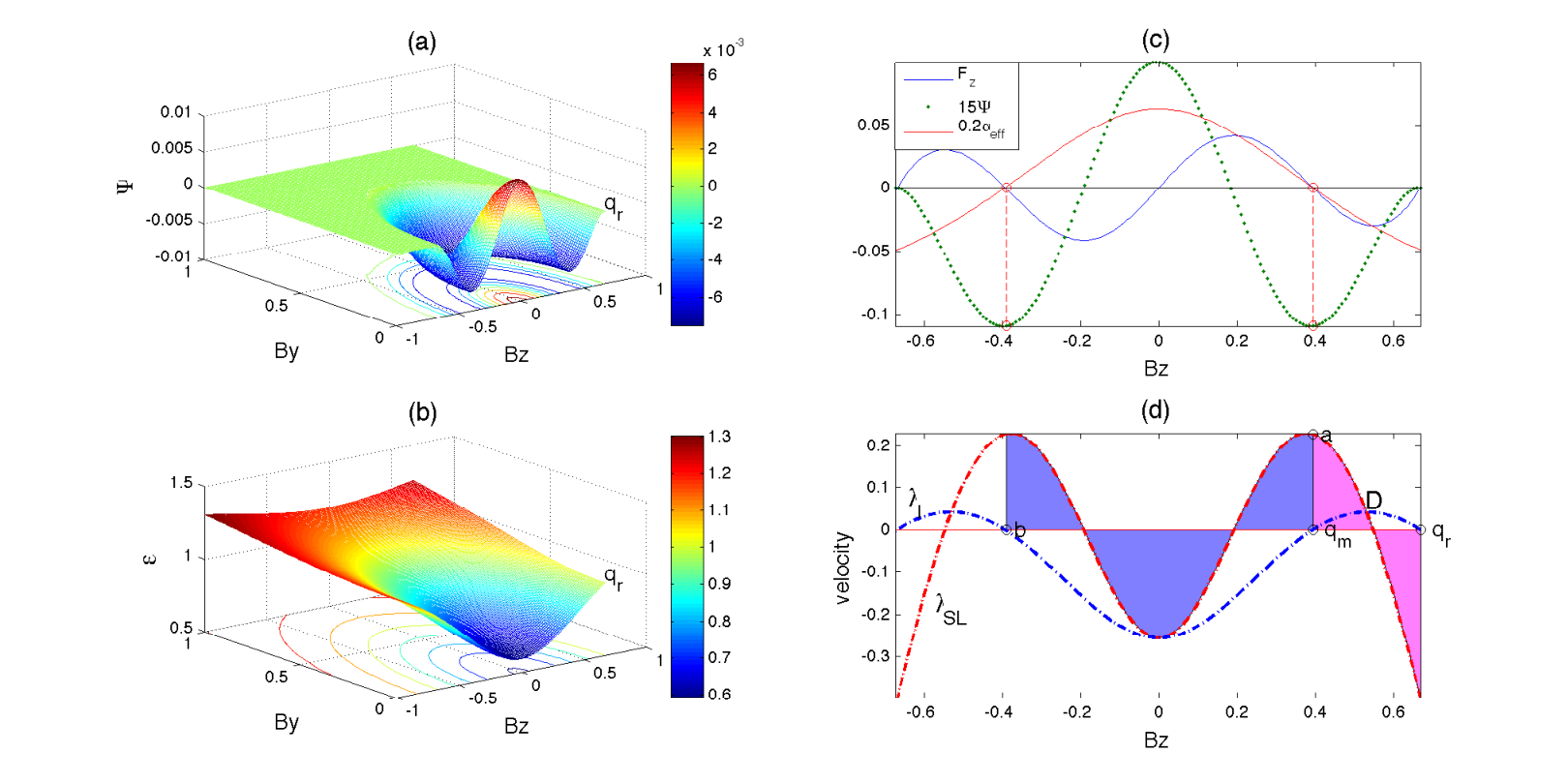
The pseudo-potential is shown in Fig. 4(a) for the parameters , , , and . The temperature anisotropy has turned the origin from a local minimum of the pseudo-potential in the isotropic MHD model to a local maximum. We term this the “reversal behavior”. A pseudo-particle initially at point will slide down the hill in the slow mode eigen-direction, and then follow the circular valley in the intermediate eigen-direction. Without the reversal behavior (e.g., in isotropic MHD) the pseudo-particle will slide down to the origin and form a switch-off slow shock. The trajectory of the pseudo-particle can also be calculated by numerically integrating Eq. (28) with respect to . In (b) the variation of the temperature anisotropy is shown. Similar reversal behaviors can be found in fully anisotropic MHD with the energy closure used here, or with the CGL closure (see Appendix IV. A).
In Fig. 4 (c), we plot a cut of the pseudo-force, , effective and the pseudo-potential along the axis (), which is the eigen-direction of a slow mode beginning at . Here
| (30) |
It is clear that occurs at in Fig. 4(c), since is constructed by integrating the pseudo-force . In Fig. 4 (d) we plot cuts of the characteristics of the slow and intermediate modes along the axis.
| (31) |
| (32) |
The temperature anisotropy has changed the structure of these characteristics. As a result, there are new degeneracy points () between slow and intermediate waves such as the point “D”. The slow characteristic shows extra nonconvexity points, where no steepening and spreading occurs (i.e., ), such as the point (the local maximum of ). This is clearer when we compare the slow characteristic here to that in the isotropic case shown in Fig. 10, where is the only degeneracy point and the nonconvexity point of the slow mode.
In order to identify the nonlinear waves determined by the route of the pseudo-particle, we apply the equal-area rule, which tells how shocks are steepened from characteristics. The equal-area rule (see Appendix V for more details) applied to shows that the sliding route (point to ) forms a slow shock. Since therefore , and thus the slow mode will steepen until the red area above the horizontal line equals the red area below . The slow shock transition immediately connects to the intermediate mode (point to , which is also from the equal-area rule on ) in the valley. The fact that both the upstream (point ) and downstream (point ) travel at the local makes the intermediate discontinuity a RD. By comparing (c) and (d), we note that the potential minimum is exactly the location of as expected and it is below the degeneracy point (). This fact is consistent with the comment in section V, which predicts that will be inside the degeneracy band. The horizontal lines and measure the propagation speed of the SS and the RD, which in this case are both zero in the upstream intermediate frame. They therefore form a compound SS/RD wave. The downstream of the slow shock (point ) is not able to connect to the slow rarefaction (SR) wave (point ) and thus not able to form a compound SS/SR, since the rarefaction is faster than the shock itself. This model gives an theoretical explanation for the possible satellite observations of compound SS/RD [21, 22], and the “compound SS/RD/SS waves” seen in hybrid simulations [24].
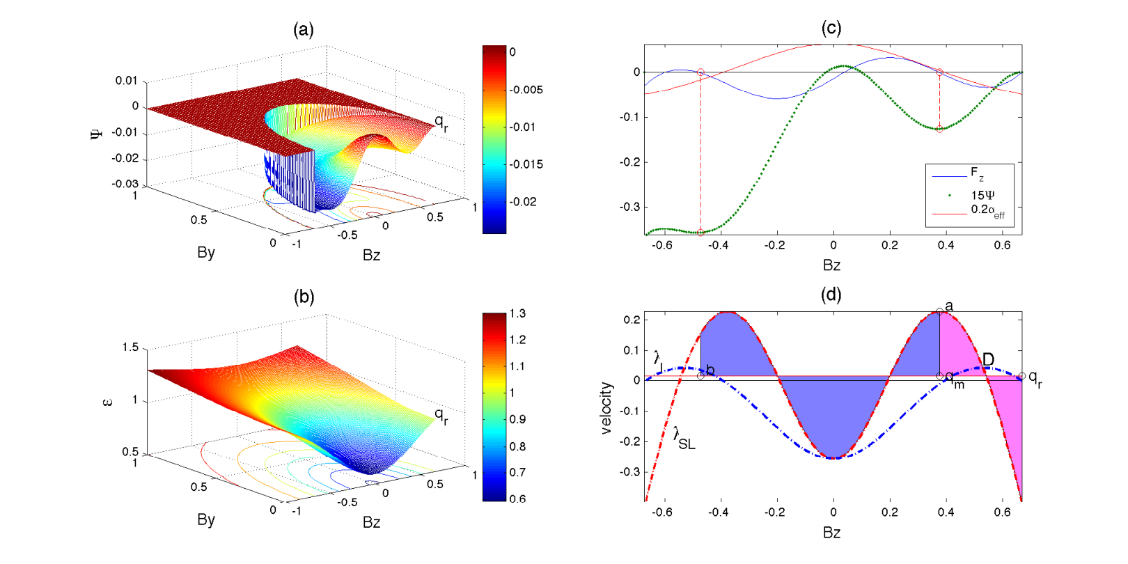
When the potential tilts down in the negative direction (see Fig. 5). In this case, the slow shock (point to in Fig. 5(d)) with shock speed is connected by an intermediate shock (IS) (point to ) with shock speed , whose upstream is super-intermediate () while the downstream is sub-intermediate (). This forms a compound SS/IS wave. Note that the intermediate shock is not steepened from the intermediate mode (which is consistent with the discussion in Sec. IV), but is steepened from the slow mode. The slow shock is abnormal with both upstream (point ) and downstream (point ) being super-intermediate. Karimabadi et al. [14] call this kind of slow shock an anomalous slow shock. When the potential tilts up in the negative direction and there is no extra transition at the SS downstream, since in this case and is therefore not accessible.
These results are independent of the details of , but only require the reversal behavior somewhere downstream of the slow shock. This fact can be inferred from a simple relation: for or , regardless of the detail of (from Eq. (30) and (32)). When , this relation ensures that the SS can always connect to a RD since at both points and . When , the SS can always connect to an IS since is positive (super-intermediate) at and negative (sub-intermediate) at . We therefore conclude that the abnormal transitions of magnetic field structures seen in the PIC simulations of Paper I are most likely the transitions from the SS to the RD in a compound SS/RD wave or the SS to the IS in an SS/IS wave. We can hardly distinguish between these two compound waves in our PIC simulation, since is small and the time-dependent dynamics add uncertainties in measuring the exact value. We focus on further analyzing the compound SS/RD wave.
VI.2 The significance of
For SS/RD waves (), the stationary points along are the roots of ,
| (33) |
Here the subscript “s” represents “stationary”. We have three traditional stationary points, (point ), and , as well as a new stationary point due to the temperature anisotropy, (the transition point ) determined by . The fixed-point analysis of the first three points in isotropic fluid theory can be found in literature [4, 8, 28, 7].
As shown in Fig. 6, there is no slow mode transition if
| (34) |
(with for monatomic plasma; note that this relation is independent of and ), which occurs when the nonlinearity of Eq. (1) changes sign from to . A positive will result in a positive in Eq. (27), and therefore no solution for . Only rotation of the magnetic field is thus allowed. If , we can further show that is always true for a slow shock transition from to in this compound wave by the full jump conditions of anisotropic-MHD (Appendix IV. B). Therefore, the nonlinear fluid theory provides a lower bound of at the SS to RD transition inside these compound waves, regardless of the details of . In other words, the downstream magnetic field cannot exhibit switch-off behavior if the firehose-sense temperature anisotropy is strong enough. This fact explains the non-switch-off slow shocks often seen in kinetic simulations [29] and satellite crossings [30]. Once it transitions to the intermediate mode, a gyrotropic will stay close to , since the intermediate-rotation nearly preserves the magnitude of the field and therefore . Note the assumption of gyrotropic is expected to be valid only in length scale larger than local ion inertial length and ion gyro-radius.
In these demonstrations we use shocks with moderate parameters, such as and . In general, larger , , and smaller will make the ratio larger, and therefore generate a stronger reversal tendency. An analysis with full anisotropic MHD (Appendix IV) should be used for strong slow shock transitions, due to the limits of the ADNLSB, although the underlying physical picture will be similar.
VII Toward the critical : time-dependent dynamics
The initial conditions that characterize the exhaust of anti-parallel reconnection (initial ) require at the symmetry line at later time. This eventually forces the pseudo-particle to climb up the potential hill to the local maximum , which implies an intrinsic time-dependent process at the symmetry line since Eq. (28) does not yield such a solution. Meanwhile, the fact that needs to go to zero at the symmetry line provides a spatial modulation on the amplitude of the rotational intermediate mode. Note that the transition point from SS to RD in compound SS/RD waves could potentially induce modulation too. As suggested in Paper I, a spatially modulated rotational wave tends to break into -scale dispersive waves, which can make the rotational component of the transition very turbulent.
As pointed out in Sec VI. B, the nonlinear fluid theory of the time-independent stationary solutions only provides a lower bound for the transition point inside these compound SS/RD waves. Counter-streaming ions, by raising , push lower. Once is lower than 0.25, the magnetic field rotates, generates -scale waves, and scatters into . This raises , changing the functional form of and driving it toward 0, which self-consistently results in a transition at the potential minimum where , and thus . This argument explains the plateau observed in the PIC simulations for different shock angles (see Fig. 1). With , this point is exactly the degenerate point of the slow and intermediate modes.
VIII The supporting evidence from numerical experiments
The evidence for a slow mode connecting to rotational waves can be seen in the PIC simulations that are discussed in detail in Paper I. In previous kinetic simulations, the downstream rotational waves were often identified as slow dispersive wavetrains arising from, for instance, the second term in the RHS of Eq. (1). Here we present further evidence, in addition to the numerical evidence that , to support the idea that the downstream rotational mode is tied to the intermediate mode. Fig. 7 shows the results from three PIC simulations that were designed to explore the structure of reconnection exhausts in the normal direction. The format is the same as for Fig. 5 of Paper I, with the first column showing , the second column the magnetic field components, and the third column a hodogram of the fields. The dashed curves in the second column (from ideal isotropic MHD [31]) indicate that a pair of switch-off slow shocks or a pair of rotational discontinuities will propagate out from the center. All three cases show the correlation between and the transition from coplanar to non-coplanr rotation of the downstream magnetic fields. The hodograms are readily comparable to the state space plots such as Fig. 2 (c). In Fig. 7(a), the downstream region of a slow shock shows a high wavenumber () left-handed (LH) polarized rotational wave, which is difficult to distinguish from the predicted downstream ion inertial scale dispersive slow mode wavetrain [6]. Fig. 7(b) shows results from a simulation with a larger initial current sheet width and exhibits a longer wavelength () LH rotational wave which can be identified as an intermediate mode The intermediate mode breaks into smaller ion inertial scale waves, which have been identified as dispersive waves in Paper I. By comparing (a) and (b), we note that the downstream primary rotational wave tends to maintain its spatial scale as an intermediate mode with non-steepening and non-spreading properties. Another way to distinguish the dispersive behavior from the non-dispersive rotation is by including a weak guide field. In Fig. 7(c), the front of the rotational downstream wave turns into a well-defined RD when a weak guide field is included. Its amplitude is about the same as that of the large amplitude rotational waves in (a). Most importantly, there is a clear slow shock ahead of the RD. Because the symmetry of the initial condition is broken by the guide field, the downstream RD does not need to end at ; instead it ends inside the potential valley at (see the hodogram of (c)), as expected.
IX Conclusion and discussion
The existence of compound SS/RD, SS/IS waves arising from firehose-sense and -correlated (temperature anisotropies) are theoretically demonstrated by analyzing the anisotropy-caused reversal of a pseudo-potential. The pseudo-potential is known to characterize the nonlinearity of hyperbolic wave equations. Extra degeneracy points between slow and intermediate modes as well as extra non-convexity points in the slow characteristics are introduced by the temperature anisotropy. The slow shock portion of a compound SS/IS wave is an anomalous slow shock with both up and downstream being super-intermediate. The nonlinear fluid theory provides a lower bound of for the SS to RD transition, regardless of the details of the energy closure . The wave generation from the rotational intermediate mode discussed here and in Paper I helps keep . This explains the critical anisotropy plateau observed in the oblique slow shock PIC simulations documented in Paper I. This study also suggests that it is a pair of compound SS/RD waves that bound the antiparallel reconnection outflow, instead of a pair of switch-off slow shocks as in Petschek’s reconnection model. This fact explains the in-situ observations of non-switch-off slow shocks in magnetotail [30]. It also provides a theoretical explanation of the observations of “Double Discontinuity” by Whang et al. [21, 22] with GEOTAIL data, and also the step-like slow shocks seen in Lottermoser et al.’s large-scale hybrid reconnection simulation [29]. In previous hybrid and PIC simulations, the downstream sharp rotational waves were often identified as slow dispersive waves of a switch-off slow shock. Instead, we propose that they are the intermediate portion of the compound SS/RD wave. The slow shock portion becomes less steep due to the time-of-flight effect of backstreaming ions.
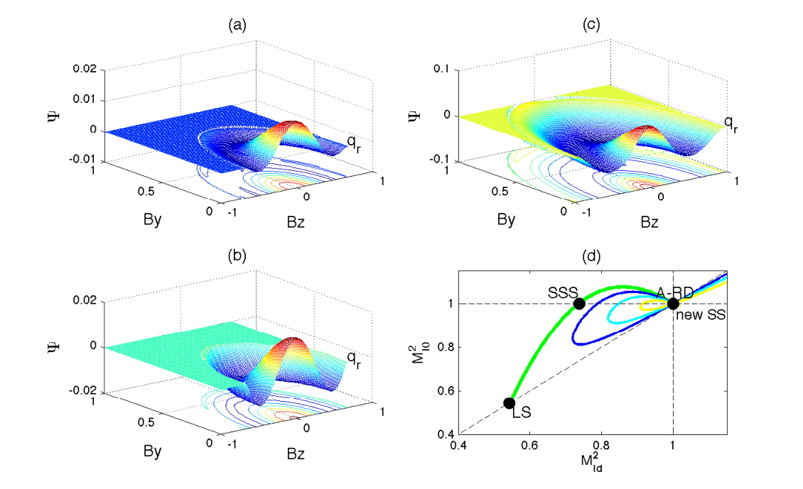
The singularity of was also noticed by P. D. Hudson [17] in his study on the anisotropic rotational discontinuity (A-RD). Unlike the RD in a compound SS/RD wave, an A-RD changes both and thermal states. Through the constraint of the positivity of , and , he derived all of the possible jumps (independent of the energy closure used) of the temperature anisotropy across an A-RD, as shown in Fig. 8(a). (Note that in Fig. 8 when .) The ADNLSB inherits most of the hyperbolic properties (such as the extra nonconvexity and degeneracy points) of anisotropic MHD and also this singular behavior. We can tell this by searching for stationary solutions where the pseudo-force (the general form of Eq. (30)). Again,
| (35) |
A stationary A-RD exists at (i.e., , and ), only if we require . An arbitrary magnetic field magnitude and rotation are then allowed, as shown by Hudson. After further constraining the possible jumps by requiring that entropy increase, the solution above the diagonal line in Fig. 8b is eliminated when while the solution below the diagonal line is eliminated when . He also noticed that the jump behavior of an A-RD for is slow-mode-like (i.e. and are anti-correlated), while it is fast-mode-like (i.e. and are correlated) for . This directly relates to the fact that the jump of an A-RD equals the jump of the compound SS/RD wave (see Appendix IV. C), and a slow mode turns fast-mode-like when [4].
X Appendices
I - From anisotropic MHD to the Anisotropic DNLSB equation:
From moment integrations of the Vlasov equation that neglect the off-diagonal components of the pressure tensor (the empirical validity of this approximation for our system is shown in Fig. 3(c) of Paper I), we can write down the anisotropic MHD (AMHD) equations [15, 16]. The energy closure is undetermined.
In Lagrangian form,
| (36) |
| (37) |
| (38) |
| (39) |
| (40) |
where
| (41) |
or for monatomic or diatomic plasma, respectively [32]. , , , , , , , , and are the temperature anisotropy factor, pressure parallel to the local magnetic field, pressure perpendicular to the local magnetic field, mass density, velocity of the bulk flow in the normal direction (), velocity of the bulk flow in the tangential direction (- plane), normal component of the magnetic field, tangential components of the magnetic field, the heat flux in the -direction and the magnetic resistivity (assumed constant). The first and the second term on the RHS of Eq. (39) are from the magnetic dissipation and the Hall term respectively.
Then we follow the procedure of Kennel et al. [4], using Lagrangian mass spatial coordinates,
| (42) |
Jumping to the upstream (subscripted by “0”) intermediate frame in order to separate the slow and fast variations, we take
| (43) |
where , and with the approximations
| (44) |
(where means variation), we can collapse the original seven equations into two coupled equations
| (45) |
with
| (46) |
and
| (47) |
where , , and .
Since the heat flux is approximately proportional to (as pointed out in Fig. 3(a) of Paper I), it should enter the source term on the RHS as . In plasmas with , is negative and hence the heat flux helps shocks dissipate energy. We implicitly incorporate it into the resistivity (as, for instance, is done for the shear and longitudinal viscosities discussed in [4]). We then arrive at the anisotropic DNLSB equation, Eq. (1). This equation can also be derived from regular reductive perturbation methods with a proper ordering scheme. For instance, a DNLS equation with the CGL condition and more corrections, including finite ion Larmor radius effects and electron pressure, was derived using regular reductive perturbation methods [33].
II - Non-steepening and non-spreading of the intermediate mode:
Beginning with the anisotropic MHD equations in Lagrangian form in Appendix I, we neglect the dissipation and the Hall term on the RHS of Eq. (39). Then the simple wave solution can be obtained by substituting , , where is the wave speed and means variation. [34]
| (48) |
| (49) |
| (50) |
| (51) |
| (52) |
| (53) |
Eq. (51) and Eq. (53) give us the intermediate speed . Combined with Eq. (48), the steepening tendency of an intermediate mode can then be expressed as,
| (54) |
Using Eqs. (48), (49), (50) and (52), we get . Therefore, the intermediate mode in anisotropic MHD does not steepen or spread, no matter what energy closure is used. It is linearly degenerate, as is its counterpart in isotropic MHD.
III -The integral curves and Hugoniot Locus:
To find the integral curves, we follow the eigenvector of the slow mode to form a curve,
| (55) |
where is a dummy variable. The integral curve is .
For the intermediate mode,
| (56) |
Therefore, the integral curve is .
As to the Hugoniot locus, we need to compute the shock speed where is the flux of Eq. (III) and or .
| (57) |
These can be combined to give,
| (58) |
The first root is the Hugoniot locus of the slow mode: . For , so that , the second root gives us the Hugoniot locus of the intermediate mode: . Although these results are the same as derived from the integral curves, this is not generally the case.
IV - The pseudo-potential of Anisotropic MHD (AMHD):
In the de Hoffmann-Teller frame, the jump conditions can be written as (following Hau and Sonnerup’s procedure [28, 7]),
| (59) |
| (60) |
| (61) |
| (62) |
where we define a jump relation , with the upstream value and the value inside the transition region. From Eq. (59)-(62), we can derive
| (63) |
where
| (64) |
| (65) |
| (66) |
with .
The generalized Ohm’s law is
| (67) |
where the first and the second term on the RHS are the magnetic dissipation and the Hall term respectively. With the final jump condition , we obtain
| (68) |
| (69) |
where measures the ratio of the dispersion to the resistivity. The pseudo-potential is uniquely defined since .
: Fig. 9(a) shows the pseudo-potential of AMHD for the same parameters as Fig. 4(a) (which was calculated based on the reduced ADNLSB formulation). If then , and thus the potential minimum (where ) occurs at . This implies that in the shock frame (also the upstream intermediate frame), at the potential minimum. This is essentially the same point (where ) of Fig. 4(d) with ADNLSB. Fig. 9(b) shows a similar reversal with the CGL closure. We note that the CGL closure exhibits an even stronger tendency to reverse the pseudo-potential. In Fig. 9(c), the pseudo-potential for , and is shown, these parameters are more similar to those seen in our PIC simulation.
: Now we consider the jump conditions to an asymptotic downstream by neglecting the LHS and terms with of Eqs. (68) and (69). The relation can be derived where we label quantities (“d” for downstream). We can eventually invert as a function of from Eq. (63). The result is plotted in Fig. 9(d) which shows possible shock solutions as functions of the downstream intermediate Mach number [14]. In the green curve ( case), the portion from A-RD (anisotropic-RD) to SSS is the IS branch, from SSS to LS (linear slow mode) is the SS branch. When , a new slow-shock transition from to is noted at the point (1,1). This new SS constitutes the slow shock portion of a compound SS/RD wave. For a given , the smallest possible shrinks the SS and IS branches to the point (1,1). It can be shown that is always true for . Therefore the existence of the new slow shock requires . In other words, is always true for a SS/RD compound wave in full anisotropic MHD.
: From Fig. 9(d) and further investigations, it can be shown that the anisotropic-RD(A-RD) at (1,1) has the same jump as that of the new SS at (1,1) plus a RD that does not change and thermal states. Therefore an A-RD and the corresponding compound SS/RD wave have the same jump relations.
V - The Equal-Area Rule and Intermediate Shocks:
The equal-area rule applies to conserved quantities in hyperbolic equations, which in our case is . From Eq. (III) and the general form of Eq. (30), we find a simple relation between the pseudo-force and the flux function,
| (70) |
From Eq. (III) and Eq. (15), a simple relation between the slow characteristic and the flux function is
| (71) |
It is then easy to show that,
| (72) |
This indicates that a stationary point , where , will be located where the integral on the LHS is zero. This is called the equal-area rule. From this relation, with a given and , we can determine the shock speed that causes the integral to vanish. Or for a given and , we can determine the possible downstream state . We apply it to the following examples to demonstrate the formation of intermediate shocks (which have a super-intermediate to sub-intermediate transition) in isotropic MHD.
When the upstream is given and fixed, we can vary to see the effect on possible shock solutions. In Fig. 10(a), when is chosen above , a slow shock solution is found by determining a proper horizontal line (; note that the vertical position measures the shock speed ), which makes the red area below the line equal the red area above. The shock speed is slower than the upstream intermediate speed (black horizontal line across 0), the upstream (point ) is super-slow and sub-intermediate (, . Since equivalents to where is the phase speed and is the bulk flow speed measured in upstream intermediate frame, implies that the mach number measured in shock frame ) and the downstream (point ) is sub-slow (). Traditionally in isotropic MHD, the super-fast state is termed number 1, sub-fast and super-intermediate is 2, sub-intermediate and super-slow is 3, and sub-slow is 4. Therefore a slow shock is also called a 3-4 SS.
In Fig. 10 (b), if is chosen below the point , a 2-4 intermediate shock () is formed, with upstream being super-intermediate and downstream being sub-intermediate and sub-slow. In Fig. 10(c), with the same shock speed, a 2-3 IS transitions to a with a more negative value is also possible. Note that the jump cross a compound 2-3 IS/ 3-4 SS (from this to the in (b) ) equals to that of the 2-4 IS in (b). In Fig. 10(d), with the same of Fig. 10(c), a 2-3=4 IS () with the maximum IS speed could be formed and attached by a slow rarefaction (). This is a compound IS/SR wave, with which can also be determined by , as shown by Brio and Wu [2]. Similar arguments can be made in a system with fast and intermediate modes.
Therefore, an intermediate shock is not directly associated with an intermediate mode. It is steepened by magneto-sonic waves (slow or fast modes), not by intermediate mode itself. This was first justified by Wu’s (1987) coplanar simulations [3] (i.e., no out-of-plane magnetic field is allowed), where the intermediate shock forms even though the intermediate mode is not included (since the out-of-plane is necessary for nontrivial solutions of the intermediate mode, as shown in Appendix II). The coupling of intermediate and magneto-sonic waves and the admissibility of intermediate shocks in the ideal MHD system was discussed by Kennel et al. [4].

References
- [1] Yi-Hsin Liu, J. F. Drake, and M. Swisdak, submitted to POP (2011).
- [2] M. Brio and C. C. Wu, J. Comp. Physics 75, 400 (1988).
- [3] C. C. Wu, Geophys. Res. Lett. 14, 668 (1987).
- [4] C. F. Kennel, R. D. Blandford, and C. C. Wu, Phys. Fluids B 2, 253 (1990).
- [5] C. C. Wu, Space Science Reviews 107, 403 (2003).
- [6] F. V. Coroniti, Nucl. Fusion 11, 261 (1971).
- [7] L. N. Hau and B. U. Ö. Sonnerup, J. Geophys. Res. 95, 18791 (1990).
- [8] C. C. Wu and C. F. Kennel, J. Plasma. Phys. 47, 85 (1992).
- [9] C. F. Kennel, J. Geophys. Res. 93, 8545 (1988).
- [10] D. W. Longcope and S. J. Bradshaw, Astrophys. J. 718, 1491 (2010).
- [11] B. Abraham-Shrauner, J. Plasma. Phys. 1, 361 (1967).
- [12] L. N. Hau and B. U. Ö. Sonnerup, Geophys. Res. Lett. 20, 1763 (1993).
- [13] D. Krauss-Varban, N. Omidi, and K. B. Quest, J. Geophys. Res. 99, 5987 (1994).
- [14] H. Karimabadi, D. Krauss-Varban, and N. Omidi, Geophys. Res. Lett. 22, 2689 (1995).
- [15] J. K. Chao, Rep. CSR TR-70-s, Mass. Inst. of Technology. Cent. for Space Res., Cambridge, Mass. (1970).
- [16] P. D. Hudson, Planetary and Space Science 18, 1611 (1970).
- [17] P. D. Hudson, Planetary and Space Science 19, 1693 (1971).
- [18] P. D. Hudson, J. Plasma Physics 17, 419 (1977).
- [19] L. Yin, D. Winske, and W. Daughton, Phys. Plasmas 14, 062105 (2007).
- [20] R. Z. Sagdeev, Reviews of Plasma Physics 4, 23 (1966).
- [21] Y. C. Whang, J. Zhou, R. P. Lepping, and K. W. Ogilvie, Geophys. Res. Lett. 23, 1239 (1996).
- [22] Y. C. Whang, D. Fairfield, E. J. Smith, R. P. Lepping, S. Kokubun, and Y. Saito, Geophys. Res. Lett. 24, 3153 (1997).
- [23] D. W. Walthour, J. T. Gosling, B. U. Ö. Sonnerup, and C. T. Russell, J. Geophys. Res. 99, 23705 (1994).
- [24] L. C. Lee, B. H. Wu, J. K. Chao, C. H. Lin, and Y. Li, J. Geophys. Res. 105, 13045 (2000).
- [25] C. F. Kennel, B. Buti, T. Hada, and R. Pellat, Phys. Fluids 31, 1949 (1988).
- [26] R. J. Leveque, Finite Volume Methods for Hyperbolic Problems (press syndicate of the U. of Cambridge, 2002), chap. 13.
- [27] C. F. Chew, M. L. Goldberger, and F. E. Low, Proc. Roy. Soc. London Ser. A 236, 112 (1956).
- [28] L. N. Hau and B. U. Ö. Sonnerup, J. Geophys. Res. 94, 6539 (1989).
- [29] R. F. Lottermoser, M. Scholer, and A. P. Matthews, J. Geophys. Res. 103, 4547 (1998).
- [30] J. Seon, L. A. Frank, W. R. Paterson, J. D. Scudder, F. V. Coroniti, S. Kokubun, and T. Yamamoto, J. Geophys. Res. 101, 27383 (1996).
- [31] Y. Lin and L. C. Lee, Space Science Reviews 65, 1 (1993).
- [32] L. N. Hau, Phys. Plasmas 9, 2455 (2002).
- [33] M. Khanna and R. Rajaram, J. Plasma. Phys. 28, 459 (1982).
- [34] A. Jeffrey and T. Taniuti, Non-linear wave propagation (Academic Press Inc., 1964), chap. 4, pp. 167–194.