Nonparametric Reconstruction of the Dark Energy Equation of State from Diverse Data Sets
Abstract
The cause of the accelerated expansion of the Universe poses one of the most fundamental questions in physics today. In the absence of a compelling theory to explain the observations, a first task is to develop a robust phenomenology. If the acceleration is driven by some form of dark energy, then, the phenomenology is determined by the dark energy equation of state . A major aim of ongoing and upcoming cosmological surveys is to measure and its time dependence at high accuracy. Since is not directly accessible to measurement, powerful reconstruction methods are needed to extract it reliably from observations. We have recently introduced a new reconstruction method for based on Gaussian process modeling. This method can capture nontrivial time-dependences in and, most importantly, it yields controlled and unbaised error estimates. In this paper we extend the method to include a diverse set of measurements: baryon acoustic oscillations, cosmic microwave background measurements, and supernova data. We analyze currently available datasets and present the resulting constraints on , finding that current observations are in very good agreement with a cosmological constant. In addition we explore how well our method captures nontrivial behavior of by analyzing simulated data assuming high-quality observations from future surveys. We find that the baryon acoustic oscillation measurements by themselves already lead to remarkably good reconstruction results and that the combination of different high-quality probes allows us to reconstruct very reliably with small error bounds.
pacs
98.80.-k, 02.50.-rI Introduction
The discovery of the accelerated expansion of the Universe little more than a decade ago [1, 2] was a major surprise. Since then, many observational efforts to understand the underlying cause have been initiated (e.g. the Baryon Oscillation Spectroscopic Survey (BOSS) [3], WiggleZ [4], the Dark Energy Survey (DES, https://www.darkenergysurvey.org/), the Large Synoptic Survey Telescope (LSST) [5]) and proposed (e.g. BigBOSS [6], the Wide Field Infrared Survey Telescope (WFIRST) [7], Euclid [8]). These efforts focus on a set of diverse cosmological probes (supernovae, baryon acoustic oscillations, clusters of galaxies, weak lensing, etc.) to combine the best possible observations in order to help solve this puzzle.
The two currently most popular explanations are a form of dark energy or a modification of Einstein’s theory of gravity on the largest observable scales. We will focus in this paper on dark energy as the cause for the accelerated expansion. The simplest way to realize a dark energy is via a cosmological constant with a dark energy equation of state . A cosmological constant, however, is not theoretically well-motivated. If we assume that the origin is due to a vacuum energy, the predicted value is incorrect at the order of . Therefore, a more natural realization of dark energy might be a dynamical field, similar to the inflaton that is believed to drive the very early rapid expansion of the Universe. Such a dynamical field, described for example by quintessence models [9], would lead to a non-constant dark energy equation of state . It is therefore one of the major aims of ongoing and upcoming dark energy missions to measure and its time variation with high accuracy. If is modeled via a simple parametrization [10, 11], current predictions for future surveys promise measurements of the constant part at the 1% level accuracy and of the leading time varying part at the 10% level. At present, the best measurements are accurate to 10% with respect to with no strong constraints on the time variation [12, 13].
With the prospect of high-accuracy measurements from supernova (SN) surveys and complementary large-scale structure probes such as baryon acoustic oscillation (BAO) surveys, it is desirable to develop an accurate reconstruction method with reliable error bars that allows us to extract the dark energy equation of state from different measurements. While the earlier focus in the field was on parametric methods [10, 11, 14], non-parametric methods are becoming more popular [15]. The major advantage of non-parametric models is that they are not biased (no assumptions are made regarding the functional form for ). A possible disadvantage might be that if the data quality is insufficient, non-parametric approaches might not provide much information about . In principle this is also an advantage: if the data does not have enough information it is better to obtain uncertain results with large error bars than a prediction which might be biased (since the functional form assumed for is incorrect) without this bias being reflected in the error bars.
In this paper, we discuss a recently-introduced reconstruction method based on Gaussian process (GP) modeling [16, 17]. A GP is a stochastic process and each realization is a random draw from a multivariate Normal distribution. It is characterized by a mean and a covariance function, that are defined by a small number of parameters. Bayesian estimation methods are used to determine the parameters of the GP model together with any other physics parameters. Therefore, the final form of the GP model is informed by the data itself. The form of the covariance function is general enough to accommodate a large variety of possible outcomes for . The only assumption made is that is somewhat smooth and continuous. If the underlying cause for the accelerated expansion is due to a physically well motivated reason this assumption is justified. We extend the approach described in detail in Ref. [16] to include different observational probes of , namely supernova measurements, cosmic microwave background (CMB) observations, and BAO results. We begin with an analysis of currently available data. We find, not surprisingly, that our predictions are in good agreement with a cosmological constant. Using simulated data, we then explore the ability to extract variations of away from a cosmological constant with improving accuracy and statistics of the data. The inclusion of the additional BAO and CMB measurements greatly help to improve these predictions.
The paper is organized as follows. In Section II we describe the different data sources included in our analysis, namely, supernova, CMB, and BAO measurements. In Section III we describe our GP model based reconstruction method. We carry out an analysis of currently available data in Section IV. We demonstrate that the method will allow us to extract variations in the dark energy equation of state by using simulated data in Section V. Finally, we conclude in Section VI.
II Dark Energy Equation of State from Diverse Data Sets
Type Ia supernova measurements are currently the best source of information regarding possible deviations of from a constant value. In the future, BAO (and other) measurements will be a strong competitor and in combination will lead to the best possible constraints on . The complementarity of the different probes is important to break degeneracies and decrease the overall errors. In our previous paper [16] we showed that our non-parametric reconstruction method is able to capture even rather sharp transitions in well if we have very good knowledge about . Supernova data alone does not provide this information and one needs a strong prior on to obtain good results. This strong prior can be justified by the existence of complementary probes. In a more direct and complete implementation, multiple probes are included in the analysis and a joint analysis is performed. This allows us to relax our prior assumptions on and to tighten our final constraints on the behavior of .
In the following, we provide a brief review of the different dark energy probes employed in this paper – supernovae, BAO, and CMB – and how to extract information about from these probes. We focus in this paper on the geometric probes for . The GP analysis is in this case very similar for all methods – is connected via two derivatives with the different distance measures. In the next section, we explain in detail how to set up a joint GP model for the three different observations.
II.1 Supernova Measurements
In this paper we retain the notation from our previous work [16]. For completeness, we summarize the important equations here. The luminosity distance as measured by supernovae is directly connected to the expansion history of the Universe described by the Hubble parameter . For a spatially flat Universe, the relation is given by
| (1) |
where is the speed of light, , the current value of the Hubble parameter (, where is the scale factor and the overdot represents a derivative with respect to cosmic time), and . The assumption of spatial flatness is in effect an “inflation prior”, although there do exist strong constraints on spatial flatness when CMB and BAO observations are combined (see, e.g., Ref. [18]). In principle, we can relax this assumption, but enforce it here to simplify the analysis.
Instead of , supernova data are usually specified in terms of the distance modulus as a function of redshift. The relation between and the luminosity distance is
| (2) | |||||
where we used Eq. (1). is the absolute magnitude of the object and the (-band) apparent magnitude. Writing out the expression for the reduced Hubble parameter in Eq. (2) explicitly in terms of a general dark energy equation of state for a spatially flat FRW Universe:
| (3) | |||||
leads to the relation
| (4) | |||
While the term proportional to (the radiation density for photons and neutrinos) is negligible at low redshift, we include it in the equations for completeness – it will become important for the CMB and BAO measurements. We use the following relation for when CMB is added to the analysis:
| (5) |
where for the standard three neutrino species, , we have and (In the following, wherever we quote values for they are quoted at .)
Note that in Eq. (4) cannot be determined from supernova measurements in the absence of an independent distance measurement. Thus can be treated as an unknown and absorbed in a re-definition of the absolute magnitude , which accounts for the combined uncertainty in the absolute calibration of the supernova data, as well as in . Using this, the -band magnitude can be expressed as where is the “Hubble-constant-free” luminosity distance (throughout this paper we will follow the convention to use capital letters for Hubble-constant-free distances and small letters for distances measured in Mpc. Different papers use different conventions.). The measurement of is only a relative measurement and allows for an additive uncertainty which can be left as a nuisance parameter. To simplify our notation, we absorb into our definition of the distance modulus, leading to:
| (6) |
With this definition of the distance modulus we have calibrated the overall offset of the data to be zero. To account for uncertainties in this calibration, we introduce a shift parameter with a broad uniform prior. The expected value for .
II.2 BAO Measurements
Baryon acoustic oscillations provide another powerful measurement of the expansion history of the Universe. Similar to supernovae they yield a geometric probe of dark energy. By carrying out measurements of the clustering along the transverse BAO scale one can obtain the angular diameter distance , defined as
| (7) |
and by measuring the BAO scale along the line of sight, one obtains information on the Hubble parameter itself (for details on future measurements, see, e.g. Ref. [6]). Both of these measurements will be carried out in terms of the sound horizon at the epoch of baryon drag, , given by:
| (8) |
and the final measurements will be in terms of and . Current data provide information only on the angular diameter distance. The structure of Eq. (7) with respect to its -dependence via two integrals is exactly the same as for given in Eq. (1). This makes it very easy to carry through a reconstruction approach combining both probes.
II.3 CMB Measurements
For the CMB measurements we employ the so-called shift parameter first introduced by Bond et al. [19]:
| (9) | |||||
where is the redshift of decoupling () and the angular diameter distance is given in Eq. (7). The shift parameter is related to the peak heights and the locations of the peaks in the temperature power spectrum of the CMB. As we will show in our analysis below, the shift parameter is very helpful in breaking the degeneracy between and when used in a combined analysis with supernova data. As an alternative to using the full CMB power spectra, the shift parameter provides a good way to summarize (see, e.g., Ref. [20]) CMB measurements, hence simplifying dark energy investigations.
One caveat of using as pointed out in, e.g., Ref. [18] is the fact that is a derived quantity from fitting to the CMB power spectrum and therefore assumes a certain cosmology. It is therefore important to state explicitly the assumption made under which the best-fit value for was derived. Several groups including Refs. [21, 20, 22] have studied this point in more detail and found that the constraints on are relatively stable under minor modifications of the dark energy parameters underlying the analysis, including dark energy clustering [22]. It was found that massive neutrinos had a larger effect on (few percent level) [22]. In Ref. [20] an analysis of WMAP-3 data was carried out and it was found that for non-flat cosmologies, the value for was very similar for different dark energy models, including constant and time-varying parametrized via . In addition, the best-fit values for in the current WMAP-7 analysis are the same within error bars for different underlying cosmologies, including CDM and open CDM models.
In our analysis of currently available data it should be kept in mind that we use the best-fit value for derived under the assumptions of a flat FRW universe with , an effective number of neutrinos of and a primordial power spectrum close to a power law. As we show below, the inclusion of in the analysis in addition to the supernova data does not alter the result for itself, its main contribution is to help relax the assumption on . For this reason, the fact that the value we use for is derived for a specific model is of much less consequence. In the case of our simulated data, the value of is obtained for the correct underlying cosmology, in which case the above discussion does not apply.
Another issue arises with the CMB measurement point due to its origin at high redshift. The SNe and BAO data points occupy a redshift range between making it easier to set up a coherent non-parametric reconstruction approach. The CMB data point on the other hand is a single point around , so far away that it is bound to cause problems for any non-parametric method. Consequently, we have to make some assumptions about the behavior of in the range – the simplest choice is .
III Reconstruction with Gaussian Process Modeling
III.1 Overview
We have recently introduced a nonparametric reconstruction method based on GP modeling and Markov chain Monte Carlo (MCMC), and applied it to supernova data [16, 17]. We refer the reader to these papers for details on the implementation of the GP model. Here, we provide a general introduction and explanation of the idea behind the reconstruction process with GP models and then focus on how to extend the method to include multiple data sources.
Gaussian processes extend the multivariate Gaussian distribution to function spaces, with inference taking place in the space of functions. The defining property of a GP is that the vector that corresponds to the process at any finite collection of points follows a multivariate Gaussian distribution. Gaussian processes are elements of an infinite dimensional space, and can be used as the basis for a nonparametric reconstruction method. Gaussian processes are characterized by mean and covariance functions, defined by a small number of hyperparameters [23]. The covariance function controls aspects such as roughness of the candidate functions and the length scales on which they can change, aside from this, their shapes are arbitrary. The use of Bayesian estimation methods (including the MCMC algorithm) allows us to estimate the hyperparameters of the GP correlation function together with any other parameters, comprehensively propagating all estimation uncertainties [24]. Using the definition of a GP, we assume that, for any collection , follow a multivariate Gaussian distribution with a constant negative mean and exponential covariance function written as
| (10) |
Here is a free parameter that, together with and the parameters defining the likelihood, are fit from the data ( and are the hyperparameters of the GP model). The form of the assumed correlation function implies that, theoretically, there is non-zero correlation between any two points. The parameter controls the exponential decay of the correlation as a function of distance in redshift, but it does not provide a bound for the correlation between two points.
The value of influences the smoothness of the GP realizations: for , the realizations are smooth with infinitely many derivatives, while leads to rougher realizations suited to modeling continuous non-differentiable functions. Here we use to allow for maximum flexibility in reconstructing . (For a comprehensive discussion of different choices for covariance functions and their properties, see Ref. [23].) We set up the following GP for :
| (11) |
The process is started using a mean value of ; given current observational constraints on this is a natural choice. Even though the mean is fixed, each GP realization actually has a different mean with a spread controlled by and the means are adjusted during the analysis to slightly different values suggested by preliminary runs (we use this strategy for some of the simulated data sets below). This adjustment is purely informed by the data and demonstrates the flexibility of the approach. In principle, the mean could also be left as a free parameter. After the adjustment we measure the posterior mean and ensure that it is close to the prior mean.
III.2 Combining Multiple Data Sources
In order to determine the optimal values for the GP modeling parameters and the cosmological parameters, we follow a Bayesian analysis approach [25]. We use MCMC algorithms to fit for the parameters [24], resulting in posterior estimates and probability intervals for and , and the hyperparameters that specify the GP model, and . We choose the following priors for the hyperparameters:
| (12) | |||||
| (13) |
Here the notation “” means “distributed according to”, and is an inverse Gamma distribution prior, with the probability density function , with . The probability distribution of the prior is given by (for examples of these distributions, see, e.g. [17]).
Turning to the cosmological parameters, we choose:
| (14) | |||||
| (15) | |||||
| (16) | |||||
| (17) | |||||
| (18) |
where is a uniform prior, with the probability density function for and otherwise. is a Gaussian (or Normal distributed) prior with the probability density function . The squared notation for the second parameter in is used to indicate that is the standard deviation (to prevent possible confusion with the variance ). (The parameters in the and distributions do not have this same meaning of mean and standard deviation as in the Normal distribution.)


The prior for for the analysis of supernova data alone is informed by the 7-year WMAP analysis [18] for a CDM model combining CMB, BAO, and measurement. Once a second cosmological probe is included in the analysis, the assumption on this prior can be relaxed and we choose a uniform prior for the analysis of the combined data sets. We also allow for an uncertainty in the overall calibration of the supernova data, , and choose a wide, uniform prior for .
| Data Type | [13] | [13] | ||||||
|---|---|---|---|---|---|---|---|---|
| SNe | -1.00 | -1 (fixed) | ||||||
| SNe+BAO | -1.07 | |||||||
| SNe+CMB | -1.00 | |||||||
| SNe+BAO+CMB | -1.01 |
Next we discuss the likelihoods for the different probes. We assume that the SNe, CMB, and BAO measurements are independent of each other which allows us to derive a likelihood for each probe separately. The likelihood for the supernova data is given by:
| (19) |
where encapsulates the cosmological parameters as well as the hyperparameters, i.e., and is the associated variance, expected to be close to unity. For the CMB data we have an equivalent expression:
| (20) |
Since we only have one data point, we cannot assign a variance parameter. The likelihood for the BAO data is slightly more complicated. For each BAO point we have two observed distance measures. These measurements are correlated and we assume that they have a correlated and bivariate Normal distribution, given by:
| (21) |
where
| (22) |
and is the associated variance parameter. This leads to the following likelihood for the BAO data:
| (23) |
with
| (24) |
We can find the combined likelihood simply by multiplying the likelihoods since we assume the different probes are uncorrelated:
| (25) |
IV Results for Current Observations
We begin our analysis by reconstructing from currently available data. We use the supernova data set recently released by Amanullah et al. [13]. This so-called Union-2 compilation (extending the Union compilation from Ref. [12]) consists of 557 supernovae between redshift and . The magnitude errors in the data set range between 0.08 and 1.02, with an average error of .
In addition to the supernova data we include the most recent BAO measurements from the Two-degree-Field Galaxy Redshift Survey (2dFGRS) at and the Sloan Digital Sky Survey (SDSS) [26] at given by
| (26) | |||||
| (27) |
where . For the CMB analysis, we use the most recent measurement of the shift parameter from WMAP-7 [18], given by
| (28) |
In order to have a complete description of the problem we have to specify some additional cosmological parameters that are expected to have little or no effect on dark energy. These parameters – fixed at the best-fit WMAP-7 values from their CDM analysis – are: , , , and .
We carry out four different analyses: supernova data by themselves with a Gaussian prior for given in Eq. (14), and combined analyses for supernova data and CMB, supernova data and BAO, and for all three probes. For the combined data sets we can relax the prior assumptions on and use a wide uniform prior, given in Eq. (15). The results are summarized in Table 1 and Fig. 1.
All results are consistent with a cosmological constant, i.e. , as can be seen in the first row in Fig. 1. The supernova data by themselves have no constraining power on and therefore force us to choose a rather strong prior. The lower panels in Fig. 1 show the prior (red line) and posterior (black line) for demonstrating this point clearly. If we include either CMB or BAO or both, the constraints on get much better. As can been seen in Table 1, the error estimates for shrink by almost a factor of two if all probes are combined. Overall, the supernova data by themselves lead to a slightly higher value of , while the combination with CMB data leads to a lower value. The inclusion of the BAO points shifts up the value for considerably, by more than 10% compared to the supernova–CMB analysis. Nevertheless, within the error bars, all values for are consistent and agree well with the best-fit WMAP-7 values including different probes. The value for the shift parameter is very close to zero in all cases.
A brief comparison with Ref. [13] also shows very good agreement. For ease of comparison, we quote their results in the last two columns of Table 1 for the case of a flat Universe and . The trends in the best-fit value for are exactly the same as we find, the value is lowest for the case of supernova+CMB data and highest for supernova+BAO data. They also find that for the supernova+BAO analysis, is slightly below while for all other cases it is very close to . Their analysis is also consistent with a cosmological constant. It is very interesting to note that our error estimates for are also very similar to the findings of Amanullah et al., even though their assumption of is very restrictive. This is very encouraging since it shows that our method leads to tight error bounds without loss of flexibility in allowing for time variations in . In contrast, a fit would have increased the error bars considerably.
V Results for Simulated Data
In this section we investigate how well our method works for reconstructing with future high-quality data. Current limitiations – uncertainties in the data and limited statistics – prevent us from extracting possible time variations in reliably. The error bands are still rather large and results are in complete agreement with a cosmological constant. Future measurements will hopefully change this: if there is a small time variation in we should be able to detect it. In our previous paper [16] we generated a supernova data set, assuming high-quality measurements from a WFIRST-like mission. We showed that a set of 2300 supernovae out to a redshift of and perfect knowledge of allows us to confidently extract time variations in the dark energy equation of state. We also showed that larger uncertainties in degraded this result due to well-known degeneracies between and . These degeneracies can be broken by including different data sources. We show in the following that a combination of accurate supernova data with results from a BAO survey such as BigBOSS will provide sufficient information to enable a reliable and interesting reconstruction of . The combination of these different data sources eliminates the degeneracy problem and provides reliable constraints on the time variation of without requiring “perfect” knowledge of .
V.1 The Simulated Data

We generate simulated data for all three probes (supernovae, BAO, CMB) and three different cosmological models. The models used are the same as in our previous work (see Ref. [16] for more details). Model 1 has a constant dark energy equation of state , Model 2 is based on a quintessence model with a minimally coupled scalar field and a dark energy equation of state , and for Model 3 we choose a slightly more extreme quintessence model with . The resulting equations of state are shown in Figure 2. For each model we choose and fix km/s/Mpc, , , , and . While Model 3 is already ruled out observationally it provides a good example for a rather sharp transition in . For each model we create two data sets: (i) We assume the best-possible scenario, a space mission to obtain supernova measurements out to redshift and in addition a BigBOSS-like BAO survey, and CMB data; (ii) good ground based supernova measurements in combination with BigBOSS and CMB measurements. In the following we provide some details on the assumptions for the different data sets.
V.1.1 Supernova Measurements
As mentioned above we investigate two different sets of simulated supernova measurements. The first one is the same as we used in Ref. [16]. It contains 2298 data points distributed over a redshift range of with larger concentration of supernovae in the midrange redshift bins () and at low redshift (). The exact distribution is shown in Ref. [16] in Fig.1. For the distance modulus we assume an error of . The measurements are presented in the following form:
| (29) |
In this notation, the observations follow a normal distribution with mean , the standard deviation being set by the distribution of the error, , representing a mean-zero normal distribution with standard deviation, . Here, is the observed error and accounts for a possible rescaling. In addition, we assume that the errors are independent.


For the second set of simulated supernova data we consider the same number of data points as currently available from ground-based surveys (557 measurements). The redshift distribution is shown in Fig. 3. The distribution extends to with a maximum at low redshift and around . Only a handful of supernovae are available at higher redshifts. Since we assume that the measurements are taken from the ground, we increase the errors on the distance modulus to . Figure 4 shows the distance modulus redshift relation of these measurements for Model 1 with error bars. The exact relations for Model 2 and 3 are shown in addition. The differences between the three models are very small, pointing to the challenge of the reconstruction task.
V.1.2 CMB Measurements
For the CMB points we use the following realizations (the exact values for for each model are given in parentheses):
| (30) | |||||
| (31) | |||||
| (32) |


V.1.3 BAO Measurements
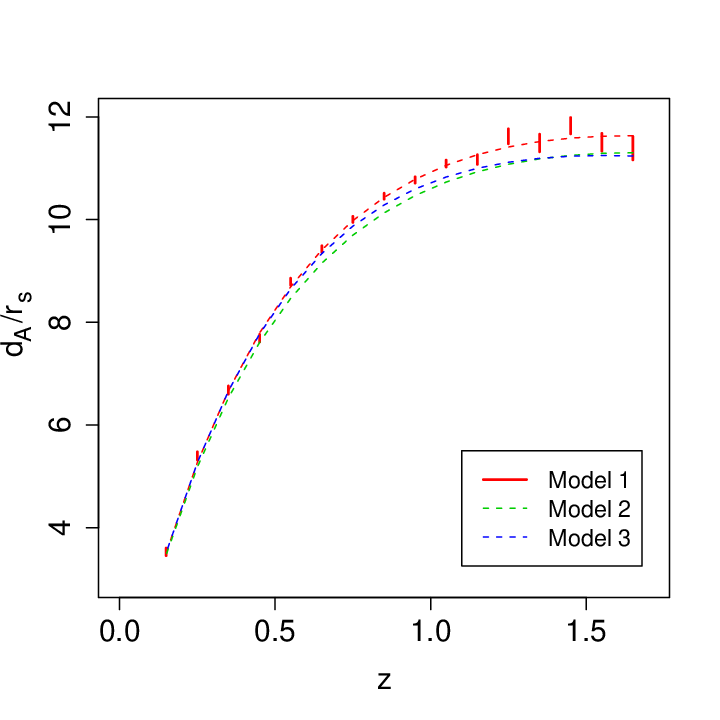
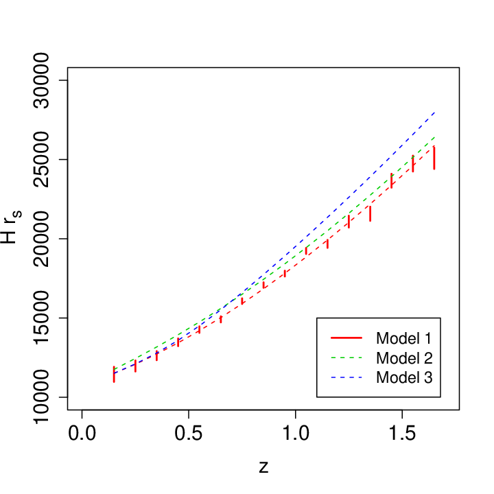
Future BAO surveys such as BigBOSS will obtain measurements of the angular diameter distance, , as well as the Hubble parameter , in terms of the sound horizon at the epoch of baryon drag, . For our simulated BAO data sets, we follow the specifications for a BigBOSS survey as outlined in http://bigboss.lbl.gov/docs/BigBOSS_NOAO_public.pdf. We assume a survey area of 24000 deg2 (covering northern and southern skies) and adopt the galaxy density distribution estimated in the BigBOSS proposal (Table 2.3 in the aforementioned document). In this proposal, measurements from luminous red galaxies and emission-line galaxies are combined. The resulting distribution accounts for several sources of inefficiency (discussed in the BigBOSS proposal) leading to a degradation of the galaxy number density at high redshift. Often, a constant galaxy density over the whole redshift range is assumed. We studied this case as well and found that the eventual results in both cases are very similar. In order to derive estimates for the errors of the simulated measurements, we use a publicly available code introduced in Ref. [28]. The formula used to obtain BAO errors in this code is a 2D approximation of the full Fisher matrix formalism. In [28], the results for the full Fisher matrix calculation and this method are shown to match well. Although these results are for CDM, they should hold for other cosmologies.
The input parameters for the code are: at the present epoch, transverse rms Lagrangian displacement, with growth factor normalized such that at high redshift, Mpc for a cosmology with at present and scaling linearly with ; line of sight rms Lagrangian displacement, with as before; and the number density ([6]). are input correctly for each model. The biggest possible source of error are the formulae used for ; these were shown to be reasonable fits to the true values in [29]. The value of given is also for the cosmology used in [29]. For a different cosmology, would obviously be different, and the simplest way to deal with this, as suggested in the paper, is to scale it linearly with . This may not be completely accurate as we use very different cosmological models but should yield a reliable estimate.


Figure 5 shows two realizations for a CDM model (Model 1) for the angular distance diameter in the left column and for the Hubble parameter in the right column. In addition, we show the exact predictions for Model 2 and 3. We use two realizations for the BAO data to demonstrate the dependence of the reconstruction as a function of realization. Because observations represent only one realization, this imposes an an irreducible limitation on the reconstruction program, whether non-parametric or not. We will return to this issue in future work.
V.2 Results
V.2.1 Prelude
Before we present our results for the combined analysis of different cosmological probes we show the constraints we obtain from the simulated BAO data alone on . The results are already remarkably good. We choose a flat prior for for this analysis.
Figure 6 shows the results for both realizations presented in Figure 5, Table 2 provides the best fit values for all three models for the left column (Realization I) and Table 3 for the right column (Realization II). For Model 1 (first row) the predictions are slightly low for the first realization but overall the results are consistent with the input model., . We verified that this result does not change considerably if the tighten the prior on . Similar trends can be seen for Model 2 and 3. We will come back to these trends later in the discussion on the results for combined data sets. The value for for realization I (Table 2) is slightly high in all cases – adding CMB measurements decreases the error on but in fact shifts the best fit values even higher. The second realization leads to values for very close to the input value for BAO measurements only, the CMB point again shifts it up slightly. The reconstruction from the BAO data only works remarkably well – in all cases the underlying model is captured within the error bars reliably.
V.2.2 Combining Different Data Sets
Next we present the results for Model 1 - 3 for several different combinations of data as discussed above:
Ground-based supernova mission (Figs. 7-9, upper rows; Table 2):
- •
557 supernovae out to ,
- •
supernovae + CMB measurement
- •
supernovae + 20 BAO points (realization I)
- •
supernova + BAO + CMB measurements
Space-based supernova mission (Figs. 7-9, lower rows; Table 3):
- •
2298 supernovae out to ,
- •
supernovae + CMB measurement
- •
supernovae + 20 BAO points (realization II)
- •
supernova + BAO + CMB measurements


| Data Type | Data | |||||||
|---|---|---|---|---|---|---|---|---|
| SNe | n/a | -1.00 | ||||||
| n/a | -0.87 | |||||||
| n/a | -1.00 | |||||||
| SNe+CMB | n/a | -1.07 | ||||||
| n/a | -0.94 | |||||||
| n/a | -0.78 | |||||||
| SNe+BAO | -1.04 | |||||||
| -0.94 | ||||||||
| -0.73 | ||||||||
| SNe+BAO+CMB | -1.05 | |||||||
| -0.95 | ||||||||
| -0.73 | ||||||||
| BAO | n/a | n/a | -1.05 | |||||
| n/a | n/a | -0.92 | ||||||
| n/a | n/a | -0.75 | ||||||
| BAO+CMB | n/a | n/a | -1.07 | |||||
| n/a | n/a | -0.95 | ||||||
| n/a | n/a | -0.74 |
| Data Type | Data | |||||||
|---|---|---|---|---|---|---|---|---|
| SNe | n/a | -1.00 | ||||||
| n/a | -0.87 | |||||||
| n/a | -0.92 | |||||||
| SNe+CMB | n/a | -1.04 | ||||||
| n/a | -0.90 | |||||||
| n/a | -0.82 | |||||||
| SNe+BAO | -0.97 | |||||||
| -0.88 | ||||||||
| -0.63 | ||||||||
| SNe+BAO+CMB | -1.00 | |||||||
| -0.90 | ||||||||
| -0.71 | ||||||||
| BAO | n/a | n/a | -1.00 | |||||
| n/a | n/a | -0.88 | ||||||
| n/a | n/a | -0.68 | ||||||
| BAO+CMB | n/a | n/a | -1.03 | |||||
| n/a | n/a | -0.92 | ||||||
| n/a | n/a | -0.70 |
As for the real data, we choose a stronger prior for in the case of analyzing supernova data only while we use a flat prior for any combination of data. Figure 7 shows the results for Model 1. The reconstruction from supernova data only works very well – the additional data points (comparing the upper and lower panel) help reduce the error bands (note that the redshift range in the lower row showing the results for 2298 supernovae extends out further) and also lead to a better estimate for with tighter error bounds, given in Tables 2, 3. The addition of the CMB point (second column in Figure 7) allows us to choose a much less strict prior on , i.e. a flat prior. Overall, the reconstruction works well with the combination of supernova and CMB measurements, the error bands on shrink considerably. The estimate for is slightly too high leading to a small overall underestimation of [we remind the reader of the degeneracy of and ]. In the third column we show the supernova+BAO analysis. In this case, both results extend to due to the BAO data at those redshifts. In the upper row, the supernova data only covers a redshift range out to , the overall result is similar to the result from the BAO data only (Figure 6) though the error bands shrink considerably. Combining all three data sets leads to even narrower error bands (fourth column). In the lower row the small downward trend from the CMB point is compensated by the small upward trend from the BAO measurements at high redshifts, leading to an almost perfect reconstruction result. In the upper row, both CMB and BAO realization have a small downward trend in which surveys in the final result. Overall, the “truth” is captured well in all cases and lies well within the error bounds. We would like to emphasize that the dark blue line in the figures only represents the mean of the reconstruction result; much more significant are the error bands themselves – these must capture the true underlying model to establish a valid approach.
The results for Model 2 and 3 are similar, shown in Figures 8 and 9. Model 2 exhibits a small time variation which could be extracted from future data. The powerful combination of all three probes can be gauged by the relatively small error bands shown in the fourth column in Figure 8. At low to intermediate redshifts (out to ) a cosmological constant is clearly disfavored. The supernova data alone would not have had enough information to disfavor at any redshift, as the error bands in this case clearly include a cosmological constant. The inclusion of high redshift supernova data improves the results somewhat, the overall reconstruction shown in the lower left corner of Figure 8 is excellent with narrow error bands. In this case, the constraints for are also very close to the input value for the theoretical model with tight error bands.
Model 3 has a rather strong variation in . While this model is observationally ruled out already, it provides a good test bed for our new approach to demonstrate that more complicated dark energy equation of states can be reconstructed. As we discussed in detail in Ref. [16] the degeneracy between and makes the reconstruction task rather difficult – the left panels in Figure 9 show the constructed from supernova data only with a Gaussian prior on . The error bars are rather wide and include a cosmological constant comfortably. The addition of the CMB point already improves the result considerably, in this case we choose a flat prior on . The best-fit value for is very close to the input value of 0.27 compared to the case where we analyze supernova data only. The inclusion of the BAO data (third and fourth column) in both cases (557 and 2298 supernova data points) improves the results even more. The time dependence is well captured and the estimate for is also very good.
Some final remarks on the content of Tables 2, 3: in addition to the results discussed above, we provide some information on the results for the combination of BAO and CMB measurements. Overall, the extra information from the CMB measurement does not help very much to improve the results, contrary to what we find when we add this information to the supernova data. In addition to the constraints on the cosmological parameters and error behavior of the data (given by for the supernova data and for the BAO data) we list the final hyperparameters for the GP model in the last three columns. Perhaps the most interesting parameter here is the adjusted mean value for given by in the last column. As we described in Ref. [16] in detail, we start the GP model with some value for (in the case of Model 1, is the natural choice for example) and run the reconstruction program for some time. The results then have information about an improved value for the mean of the GP model and the analysis framework can be adjusted accordingly. As can be seen in the Tables, the final values for are close to the mean value of the underlying truth. Because the adjustment scheme works extremely well, we started basically all reconstruction evaluations at , the GP model automatically suggesting better mean values if the choice was non-optimal. Overall, the reconstruction of works very well when multiple sources are included.
VI Conclusion
In this paper we have introduced a new non-parametric reconstruction scheme for the dark energy equation of state combining multiple cosmological probes. The reconstruction scheme is based on a GP modeling approach and provides very good constraints on with reliable error bars. The basic method was introduced in Ref. [16] for supernova data only. Here we extend the methodology to include BAO and CMB measurements. We have carried out an analysis of currently available data and found excellent agreement with a cosmological constant consistent with a large number of recent publications, including Refs. [12, 13, 26, 18, 27]. We have also demonstrated our method on simulated data for different cosmological models. In all cases, the GP model approach performed very well.
An important aspect of our new approach (as stressed in Refs. [16, 17]) is the simultaneous constraint of the cosmological parameters as well as the hyperparameters of the GP model from the data. In comparison to parametric approaches, our new method is more flexible and can therefore capture even subtle time variations in if the data quality is good enough. It produces narrow error bands over the full redshift ranges considered. For a more detailed comparison with parametrized methods, see Ref. [16].
The combination of different data probes mitigates the problem of degeneracies between and as to be expected. An encouraging observation is that even the BAO data alone (of high quality from a BigBOSS-like survey) can deliver good constraints on the time dependence of the dark energy equation of state, clearly competitive with space based supernova observations.
Our new non-parametric reconstruction approach lends itself to analysis of the promise of future dark energy probes in a reliable way. For example, possible tension in the data due to e.g. insufficient understanding of systematic errors would lead to an increase in the error bands when combining different probes (a different attempt to solve this problem with parametric methods is discussed in e.g. Ref. [30]). The GP based approach can therefore help to optimize future dark energy missions.
Acknowledgements.
We would like to thank the Institute for Scalable Scientific Data Management for supporting this work. Part of this research was supported by the DOE under contract W-7405-ENG-36. UA, SH, KH, and DH acknowledge support from the LDRD program at Los Alamos National Laboratory. KH was supported in part by NASA. SH and KH acknowledges the Aspen Center for Physics, where part of this work was carried out. We would like to thank Andreas Albrecht, Eric Linder, Adrian Pope, Martin White, and Michael Wood-Vasey for useful discussions.References
- [1] A. G. Riess et al. [Supernova Search Team Collaboration], Astron. J. 116, 1009 (1998) [arXiv:astro-ph/9805201].
- [2] S. Perlmutter et al. [Supernova Cosmology Project Collaboration], Astrophys. J. 517, 565 (1999) arXiv:astro-ph/9812133].
- [3] D. Schlegel, M. White, and D. Eisenstein, arXiv:0902.4680 [astro-ph.CO]
- [4] M. J. Drinkwater et al., Mon. Not. Roy. Astron. Soc. 401, 1429 (2010) [arXiv:0911.4246 [astro-ph.CO]].
- [5] LSST Science Book, Version 2.0. [LSST Science Collaborations and LSST Project Collaboration], arXiv:0912.0201 [astro-ph.IM].
- [6] D. J. Schlegel et al., arXiv:0904.0468 [astro-ph.CO].
- [7] N. Gehrels, arXiv:1008.4936 [astro-ph.CO].
- [8] A. Refregier, A. Amara, T. D. Kitching, A. Rassat, R. Scaramella, J. Weller and f. t. E. Consortium, arXiv:1001.0061 [astro-ph.IM].
- [9] C. Wetterich, Nucl. Phys. B 302, 668 (1988); B. Ratra and P.J.E. Peebles, Phys. Rev. D 37, 3406 (1988); P.J E. Peebles and B. Ratra, Astrophys. J. 325, L17 (1988); R. R. Caldwell, R. Dave and P. J. Steinhardt, Phys. Rev. Lett. 80, 1582 (1998) .
- [10] M. Chevallier and D. Polarski, Int. J. Mod. Phys. D 10, 213 (2001) [arXiv:gr-qc/0009008].
- [11] E. V. Linder, Phys. Rev. Lett. 90, 091301 (2003) [arXiv:astro-ph/0208512].
- [12] M. Hicken et al., Astrophys. J. 700, 1097 (2009) [arXiv:0901.4804 [astro-ph.CO]].
- [13] R. Amanullah et al., Astrophys. J. 716, 712 (2010) [arXiv:1004.1711 [astro-ph.CO]].
- [14] A.R. Cooray and D. Huterer, Astrophys. J. 513, L95 (1999) [arXiv:astro-ph/9901097]; I. Maor, R. Brustein and P.J. Steinhardt, Phys. Rev. Lett. 86, 6 (2001) [Erratum-ibid. 87, 049901 (2001)] [arXiv:astro-ph/0007297]; J. Weller and A.J. Albrecht, Phys. Rev. Lett. 86, 1939 (2001) [arXiv:astro-ph/0008314].
- [15] R.A. Daly and S.G. Djorgovski, Astrophys. J. 597, 9 (2003) [arXiv:astro-ph/0305197]; D. Huterer and A. Cooray, Phys. Rev. D 71, 023506 (2005) [arXiv:astro-ph/0404062]; C. Zunckel and R. Trotta, Mon. Not. Roy. Astron. Soc. 380, 865 (2007) [arXiv:astro-ph/0702695]; C. Clarkson and C. Zunckel, Phys. Rev. Lett. 104, 211301 (2010) [arXiv:1002.5004 [astro-ph.CO]].
- [16] T. Holsclaw, U. Alam, B. Sanso, H. Lee, K. Heitmann, S. Habib and D. Higdon, Phys. Rev. D 82, 103502 (2010) [arXiv:1009.5443 [astro-ph.CO]].
- [17] T. Holsclaw, U. Alam, B. Sanso, H. Lee, K. Heitmann, S. Habib and D. Higdon, Phys. Rev. Lett. 105, 241302 (2010) arXiv:1011.3079 [astro-ph.CO].
- [18] E. Komatsu et al. [ WMAP Collaboration ], Astrophys. J. Suppl. 192, 18 (2011) [arXiv:1001.4538 [astro-ph.CO]].
- [19] J. R. Bond, G. Efstathiou and M. Tegmark, Mon. Not. Roy. Astron. Soc. 291, L33 (1997) [arXiv:astro-ph/9702100].
- [20] Y. Wang and P. Mukherjee, Phys. Rev. D 76, 103533 (2007) [arXiv:astro-ph/0703780].
- [21] O. Elgaroy and T. Multamaki, Astron. & Astrophys. 471, 65 (2007) [arXiv:astro-ph/0702343].
- [22] P. S. Corasaniti and A. Melchiorri, Phys. Rev. D 77, 103507 (2008) [arXiv:0711.4119 [astro-ph]].
- [23] S. Banerjee, B.P. Carlin, and A.E. Gelfand, Hierarchical Modeling and Analysis for Spatial Data, New York: Chapman and Hall (2004); C.E. Rasmussen and K.I. Williams, Gaussian Processes for Machine Learning, Boston: MIT Press (2006).
- [24] D. Gamerman and H.F. Lopes, Markov Chain Monte Carlo: Stochastic Simulation for Bayesian Inference, New York: Chapman and Hall (2006).
- [25] A. Gelman, B. Carlin, H. Stern, and D. Rubin, Bayesian Data Analysis, New York: Chapman and Hall (2004).
- [26] W.J. Percival et al., Mon. Not. Roy. Ast. Soc. 401, 2148 (2010) [arXiv:arXiv:0907.1660 [astro-ph]].
- [27] Y. Wang, Phys. Rev. D 80, 123525 (2009) [arXiv:0910.2492 [astro-ph.CO]].
- [28] H-J. Seo and D. J. Eisenstein, Astrophys. J 665, 14 (2007) [astro-ph/0701079].
- [29] D. J. Eisenstein, H-J. Seo, and M. White, Astrophys. J. 664, 660 (2007) [astro-ph/0604361]..
- [30] C. Escamilla-Rivera, R. Lazkoz, V. Salzano and I. Sendra, arXiv:1103.2386 [astro-ph.CO].