Equivalence between classical and quantum dynamics. Neutral kaons and electric circuits

Recently, Rosner [1] (see also [2]) has proposed an interesting analogy between the physics of the weak decay of neutral K-mesons (kaons) and a classical system of oscillators either electrical or mechanical. The proposal in [1] makes use of an electric network composed by two subnetworks of L$-$C oscillators connected through a simple quadripole (two-port network).

The analogy in form pointed out in [1] is based upon the observation that the characteristic matrix of the circuit has a similar aspect to that of the effective Hamiltonian of the neutral kaon system. Afterwards in [3], an extension to a general quadripole interaction between L$-$C subnetworks was presented. The general idea of our work is to formalize the previous analysis and to extend the character of that observation going beyond an analogy, and to present an equivalence, stricto sensu, between the $\mathrm{Schr\ddot{o}dinger}$ dynamics of a quantum system with a finite number of basis states [4] and a classical dynamics. The equivalence we present is an isomorphism that connects in univocal way both dynamical systems.

We base our conclusions on the concept of ^‵equivalent dynamics$\textquoteright$ defined starting from general mathematical concepts [5], [6]. Since the $\mathrm{Schr\ddot{o}dinger}$ dynamics is defined on a complex space, while the classical dynamics of interest implies real evolution equations, we profit from the decomplexification concept that allows one to work in a common space [5]-[6]. In this way we are able to define the general class of classical $\mathcal{C}$ and quantum $\mathcal{Q}$ systems where the equivalence is valid and simultaneously, we build up the isomorphism $\Phi_{S}$, mapping $\mathcal{C}$ into $\mathcal{Q}$ that includes the general correspondence between states of both systems. After this formal development, we treat the particular case of neutral kaons system, denoted by $\mathcal{K}^{\mathrm{o}}$ ($|\mathrm{K^{o}}\rangle$ and $|\bar{\mathrm{K}}^{\mathrm{o}}\rangle$), that belongs to the general case of quantum systems $\mathcal{Q}$, particularly interested in the aspects of Charge Conjugation-Parity, $\mathrm{CP}$, invariance [7]. In the context of validity of $\mathrm{CPT}$ symmetry [8]-[9]-[10], we then consider the equivalent analysis of Time Reversal, $\mathrm{T}$, invariance.

Just to be self-contained we include a brief summary of the electric network formalism [11] we need. By making use of the concept of circuital duality [11]-[12], it was possible to obtain two equivalent electrical representations of the same classical differential equation, a fact that facilitates enormously the choice of the parameters that govern the equivalence of $\mathrm{CP}$ or $\mathrm{T}$ violation in the network. This class of electric networks $\mathcal{R}$ is univocally related to the kaon system $\mathcal{K}^{\mathrm{o}}$ because we find the complete map between the matrix elements of the effective Hamiltonian of kaons and those elements of the classical dynamics of the networks. Moreover, there exists a one to one relationship between the states $|\mathrm{K^{o}}\rangle$ and $|\bar{\mathrm{K}}^{\mathrm{o}}\rangle$ and port voltages, or currents, of the electric network.

Following these lines we can give a formal classical test of the $\mathrm{CP}$ invariance that is a reflection of the quantum test. From this test, together with the concept of dual network, one concludes that any violation of the $\mathrm{CP}$ (or $\mathrm{T}$) symmetry is directly related to the non-reciprocity of the network [1]. In fact, the observable associated to the violation of $\mathrm{T}$ invariance at the quantum level is associated to the conductance of a non-reciprocal element needed to be included in the network, the gyrator. The gyrator is a two-port, non-reciprocal, passive network without losses, and violates the classical symmetry $\mathrm{T}$ [11]-[12]-[13]. In this way, we end up with a network completely equivalent to the kaon system, that allows one to present the relevant parameters of the quantum system in terms of circuit parameters. The interaction between both L$-$C subnetworks gives rise to a shift in the proper initial free frequencies, in the same way as the masses of kaons. Moreover, the presence of proper relaxation times of the circuit are associated to the mean lives of K-short and K-long.

In Section 2 we analyze the equivalence between quantum and classical dynamics. Section 3 is devoted to the neutral kaon system, while Section 4 contains a brief account of electric networks. The correspondence between those systems is presented in Section 5. Finally in Section 6 we state our conclusions.

It is well known that two systems of equations $\mathbf{\dot{X}}(t)=\mathbf{AX}(t)$, $\mathbf{\dot{Y}}(t)=\mathbf{BY}(t)$ are linearly equivalent iff the corresponding system matrices $\mathbf{A}$ and $\mathbf{B}$ are related through a similarity transformation, namely $\mathbf{B}=S^{-1}\mathbf{A}S$ [6]. We note this equivalence relation as $\mathbf{A}\sim\mathbf{B}$ and is defined through a linear application $\Phi_{S}(\mathbf{A})$=$S^{\mathrm{-1}}\mathbf{A}S=\mathbf{B}$. In summary, fixing a matrix $S$, the application $\Phi_{S}$ is an isomorphism.

Consequently, for our purposes of connecting classical and quantum systems, it is necessary for both of them to be defined in spaces of finite dimensions. In general, a classical system $\mathcal{C}$ with $m$ degrees of freedom has its states defined on a real differential manifold [14]-[15] of dimension $m$ whereas a quantum system $\mathcal{Q}$ with $n$ states belongs to a complex Hilbert space of dimension $n$. This implies that the relationship between these systems could be not trivial. In fact, one has to profit from the so called decomplexification procedure [6] that we briefly remember here.

To every matrix $\mathbf{A}\in\mathbb{C}^{n\times n}$, the application $\boldsymbol{\nu}:\mathbb{C}^{\mathrm{\textit{n}x\textit{n}}}\longrightarrow\mathbb{R}^{\mathrm{2\textit{n}\,x\,2\textit{n}}}$ is called matrix decomplexification

Clearly, for the case $n$=1 (a complex number z) one has $\boldsymbol{\nu}(z)=\left(\begin{smallmatrix}\Re(z)&-\Im(z)\\ \Im(z)&\Re(z)\end{smallmatrix}\right)$, here $\Re(z)$ and $\Im(z)$ stand for real and imaginary part of complex number $z$ respectively.

This application $\boldsymbol{\nu}$ has several properties that are used below in our analysis. These properties can be extended to the case of complex matrices $\forall\,M,N,\in\mathbb{C}^{n\times n}$

giving rise to $\boldsymbol{\nu}([M,N])$=$[\boldsymbol{\nu}(M),\boldsymbol{\nu}(N)]$, then $[M,N]=0\Leftrightarrow[\boldsymbol{\nu}(M),\boldsymbol{\nu}(N)]=0$. In particular these properties are valid for complex numbers. The symbol $[\bullet,\star]$ is a binary operation named commutator, defined under the set of square matrices.

A way to find the similarity transformation between both systems is to take both matrices A and B to a diagonal form or in the general case to the Jordan form that always exists.

With this material we are ready to establish the equivalence between classical and quantum systems, the base of our arguments.

We are particularly interested in the quantum system of neutral kaons, denoted by $\mathcal{K}^{\mathrm{o}}$, because, under the hypothesis of Wigner-Weisskopf [20], it can be written as a two-state system. This allows one to exemplify very easily the equivalence with a classical system. Moreover, we want to give a formal context to the Rosner [1] and Cocolicchio [3] proposals to establish an analogy of the kaon system with electric networks.

General principles on the basis of the Quantum Field Theory guarantee the validity of the CPT symmetry in Nature [21]-[22]-[23]-[24]. When CPT is a symmetry, the mass of a particle and its antiparticle has to be equal [7]. This equality is experimentally verified in the case of neutral kaons in an impressive way [8]-[9]-[10]:

Consequently, in this context, it is equivalent to speak about CP or T invariance, or non-invariance.

We consider here the weak decay of the neutral kaons $\mathrm{K}^{\circ}$, $\mathrm{\bar{K}}^{\circ}$ in the standard formalism [25] that includes the strangeness selection rule $\Delta$S=$\pm$1.

All the elements of the Hilbert space $\mathcal{H}$ are eigenstates of $\mathbf{\hat{H}_{o}}=\mathbf{\hat{H}_{s}}+\mathbf{\hat{H}_{\gamma}}$ where $\mathbf{\hat{H}_{s}}$ and $\mathbf{\hat{H}_{\gamma}}$ stand for the strong and electromagnetic interactions respectively. To this one adds the small perturbation of the weak interaction $\mathbf{\hat{H}}_{w}$, that gives rise to transitions among the states of $\mathbf{\hat{H}_{o}}$.

In order to formalize the quantum dynamics we split the Hilbert space into the direct sum $\mathcal{H}=\mathcal{A}\oplus\mathcal{B}$, where $\mathcal{A}$ corresponds to the states of $\mathrm{K}^{\circ}$ and $\mathrm{\bar{K}}^{\circ}$ while $\mathcal{B}$ includes all the possible decay final states. We call $\{|j\rangle\}$ and $\{|\beta\rangle\}$ orthogonal complete basis of $\mathcal{A}$ and $\mathcal{B}$ respectively.

Consequently, any state at time $t$ is represented by

where $\underset{\beta}{\text{\LARGE{S}}}$ is a sum on $\mathcal{B}$ states.

Defining now $a_{j}(t):=\langle j|\Psi(t)\rangle$, with $j$=1,2 corresponding to $\mathrm{K}^{\circ}$ and $\bar{\mathrm{K}}^{\circ}$ respectively, and $c_{\beta}(t):=\langle\beta|\Psi(t)\rangle$ one can describe the subdynamics on $\mathcal{A}$ by the coordinates $a_{j}(t)$ or, equivalently, by considering the one to one correspondence $|\mathrm{K}^{\circ}\rangle\longleftrightarrow(1,0)^{\intercal}$, $|\bar{\mathrm{K}}^{\circ}\rangle\longleftrightarrow(0,1)^{\intercal}$, the $\mathbb{C}^{2}$ vector

also describes the same dynamics.

Just to complete the description it is necessary to give the initial condition for the evolution that is written as $a_{j}(0)\neq 0$, $c_{\beta}(0)=0$, or in other words $|\Psi$(0)$\rangle\in\mathcal{A}$.

The evolution equation of the dynamics under consideration described by $\psi(t)$ is [7]:

where $\mathbf{M}$ and $\mathbf{\Gamma}$ are hermitian matrices. Clearly, the matrix $\boldsymbol{\Gamma}$ takes into account the decay width.

All the information on the decay channels is contained in (25) as is clear from the matrix elements of $\mathbf{M-\imath\Gamma}$:

with $E_{j}$ and $E_{\beta}$ being the eigenvalues of $\mathbf{\hat{H}_{o}}$ associated to the basis states.

When the Hamiltonian $\mathbf{\hat{H}}$ has a given symmetry, there exist relations among the matrix elements $\mathbf{H=M-\imath\Gamma}$.

In [7] we see that if CPT is a symmetry, one has $\mathrm{M}_{11}=\mathrm{M}_{22}$ and $\mathrm{\Gamma}_{11}=\mathrm{\Gamma}_{22}$, while if T is also a symmetry, then $\mathrm{M}_{12}=\mathrm{M}_{21}$ and $\mathrm{\Gamma}_{12}=\mathrm{\Gamma}_{21}$.

In other words, the symmetry, when projected in the subspace $\mathcal{A}$, provides relationships among the matrix elements of $\mathbf{H}$ and consequently provides a test of violation.

Before the crucial experiment [26] everything pointed to $\mathbf{CP}$ as a good symmetry. This implied that, with the election of the phases of the states $\{|\mathrm{K^{o}}\rangle,|\mathrm{\bar{K}^{o}}\rangle\}$ in such a way that $\mathbf{\hat{C}\hat{P}}|\mathrm{K^{o}}\rangle=|\mathrm{\bar{K}^{o}}\rangle$ [24], one can write states with well defined CP, given naturally as the mixtures $|\mathrm{K_{1}}\rangle=\tfrac{|\mathrm{K^{o}}\rangle+|\mathrm{\bar{K}^{o}}\rangle}{\sqrt{2}},\>|\mathrm{K_{2}}\rangle=\tfrac{|\mathrm{K^{o}}\rangle-|\mathrm{\bar{K}^{o}}\rangle}{\sqrt{2}}$, obtained through the change of basis given by the unitary matrix

that diagonalizes the Hamiltonian $\mathbf{H=M-\imath\Gamma}$.

CP being conserved, the only decays into pions allowed are $|\mathrm{K_{1}}\rangle\longmapsto|2\pi\rangle,\>|\mathrm{K_{2}}\rangle\longmapsto|3\pi\rangle$ because the states $|2\pi\rangle$ and $|3\pi\rangle$ have well defined CP, namely $\mathbf{\hat{C}\hat{P}}|2\pi\rangle=|2\pi\rangle$ and $\mathbf{\hat{C}\hat{P}}|3\pi\rangle=-|3\pi\rangle$ [7]-[27]. These two decay modes have certainly very different decay times. In fact, the first one has $\tau$ of the order of $10^{-10}s$ while the second is of the order of $5\times 10^{-8}s$.

An electric network [11]-[12] includes a set of elements together with a given way of connections among them. These elements can be classified into five classes, namely: resistors {R}, capacitors {C}, inductances {L}, voltage generators {$v_{g}$} and current generators {$i_{g}$}. We are particularly interested in localized circuits where voltage and current depend only upon time. The standard linear relations among the classes are

The way that the elements are connected is determined by a linear graph, defined by nodes connected by edges. When the edges have a given sense, provided by the current flowing through it, one says that the graph is oriented, and each edge of the graph is called arc. The oriented graph $\mathcal{G}$ is noted by means of a cartesian product of the sets of nodes and arcs $\mathcal{G=(N,A)}$. We are interested in connected graphs, those where there is at least one path of $\mathcal{G}$ between any pair of nodes of $\mathcal{G}$.

The corresponding dynamics of an electric network is defined by the appropriate use of the relations (31) together with the Kirchhoff rules that take care of the topology of the network.

The network has ports: pairs of terminals that allow exchange of energy with the surrounding. We restrict our analysis to passive networks, where the energy provided by an external source is non-negative. In any case one has the possibility of choosing the voltage or the current as the representative variable of the excitation or of the response of the network.

We call v$(t)$ the vector corresponding to the port voltage and V$(s)$ its Laplace transform. A similar notation is used for currents, i$(t)$ and I$(s)$ respectively. The network, initially without external energy, provides the relation

between the Laplace transform of the output $\boldsymbol{\mathcal{O}}$ and the input $\boldsymbol{\mathcal{J}}$ [11]. Consequently, $\boldsymbol{\mathcal{M}}$ is the network matrix.

From $\mathcal{O}_{\alpha}(s)=\sum_{\beta=1}^{n}\mathcal{M}_{\alpha\beta}(s)\mathcal{J}_{\beta}(s)$ there results

given rise to the definition of the elements of

where $r_{\alpha}$ and $e_{\beta}$ stand for response and excitation, respectively. One then says that the network $\mathcal{R}$ has a $\mathcal{M}$-representation or that it belongs to the class $\mathcal{M}$.

When the port voltages can be considered as input and the port currents as output, the corresponding representation of the network is called of admittance or type $\mathbf{Y}$, and the input-output relationship is

On the other hand, if the port currents are chosen as input and the port voltages as output, one is in the case of the impedance representation or type $\mathbf{Z}$. In this case one has

Any other representation is called hybrid.

A very important concept, relevant to our discussion is that of reciprocity. A network not connected to external energy sources is reciprocal iff considering two different terminals $\alpha$ $\neq$ $\beta$, the excitation in $\alpha$ gives rise to a response in $\beta$ that is invariant under the permutation $\alpha\longleftrightarrow\beta$ or $e_{\alpha}(t)=e_{\beta}(t)\Longrightarrow r_{\alpha}(t)=r_{\beta}(t)$.

Consequently, $\mathcal{R}$ is reciprocal iff $\mathcal{M}_{\alpha\beta}(s)=\mathcal{M}_{\beta\alpha}(s)$ with $\alpha$ $\neq$ $\beta$.

The diagonal elements {$\mathcal{M}_{\alpha\alpha}$} are called of input ones, because they relate the quantities of port $\alpha$, while the elements not belonging to the diagonal {$\mathcal{M}_{\alpha\beta}$}, with $\alpha\neq\beta$ are called of transference ones, and relate quantities of different ports.

The main goal of our proposal is to build an electric circuit able to describe the system of neutral kaons, satisfying the equivalence $\thicksim$ previously introduced. As a result, the matrix elements of the effective Hamiltonian $\mathbf{M-\imath\Gamma}$ are related, by means of a similitude transformation to those of the appropriate electric circuit as

In this way, the symmetries present in the kaon system and the corresponding tests of validity, have an unique reflection in the electric circuit.

The method of analysis of the time evolution of electric circuits previously introduced, based on nodes, arcs and loops [11] ends on a system of linear differential equations of second order with constant coefficients, or alternatively on systems of linear integro-differential equations. In our case, as the precise electric network is not known, one has to make a synthesis [11] of the set of all electric networks in a given family or subset of this.

The general scheme of the procedure is to look for the network that is equivalent to a quantum system of n-states. This network should have a first order equivalent equation of the form (3), where the generalized coordinates $\{q_{j}\}$ are now voltages and currents and with the $\complement$ matrix having n eigenvalues in the third quadrant of the complex plane, together with their complex conjugates.

One ends with a general structure composed by n-subnetwork (dipoles) {$\mathcal{R}_{j}$}_j=1,…,n connected among themselves by means of the so called interaction network $\mathcal{R_{I}}$ of n ports [11]. Each subnetwork introduces a degree of freedom described by a port voltage, or port current. These time functions provide the entire information of the state $\mathcal{R}_{j}$ at a given time. Clearly, on each dipole one gives the initial condition. Figure 1 shows the resulting general topological array.

Notice that in our case, the network dynamics must be time translation invariant, as required by (3), to be in agreement with the corresponding property of the quantum system.

In general, a network of n ports allows $(2n)!/(n!)^{2}$ representations. However, only two of them are useful for our purposes, namely those where the mix of state variables is not present: all port variables are either voltages or currents. Consequently, the equivalent network families of interest are type Y or type Z.

The electric network $\mathcal{R}$ of interest in connection with the neutral kaon system should have a classical matrix $\complement$ of $4\times 4$ with two different complex eigenvalues placed on the third quadrant. Then the general topology reduces to the one composed by two subnetworks $\mathcal{R}_{1}$ and $\mathcal{R}_{2}$ connected by means of a two-port network $\mathcal{R_{I}}$, Fig. 2.

In order to fix the structure of each $\mathcal{R}_{j}$ one starts by observing that the free states (when $\mathcal{R_{I}}$ is not connected) correspond to $\mathbf{Y}(s)=\mathbf{0}$ or to $\mathbf{Z}(s)=\mathbf{0}$ according to the equations (35) and (36), respectively. Correspondingly, the free states of the quantum system of kaons are those that evolve with $\mathbf{\hat{H}}=\mathbf{\hat{H}_{o}}$ and have the form $\psi_{\circ j}(t)=\mathrm{A}_{j}e^{-\imath m_{j}t}$ of frequency $m_{j}$. This condition implies that each $\mathcal{R}_{j}$ should be reactive, i.e., without resistive losses, contributing with one proper frequency each. This condition forces one, and only one, connection of inductors and capacitors, depending on the use of voltage or current as the input. In Fig. 3 the possible subnetworks $\mathcal{R}_{j}$, $j=1,2$ that should be connected to the ports 1 and 2 of $\mathcal{R_{I}}$ are shown. Both dipoles are certainly oscillators with the corresponding frequencies dictated by the values of L_j and C_j.

It is worth noticing that if a network $\mathcal{R}$ having a dual representation $\mathcal{R}^{*}$, presents an analogous behavior (equivalent according to $\boldsymbol{\Phi}_{S}$) to a quantum system $\mathcal{Q}$ then, $\mathcal{R}^{*}$ shares this analogous behavior to $\mathcal{Q}$, i.e.

that follows from the property $\mathcal{R}\thicksim\mathcal{R}^{*}$ and the transitivity of the equivalence $\thicksim$.

Our analysis uses port voltages as excitation variables. Then the complete network can be schematized as in Fig. 4

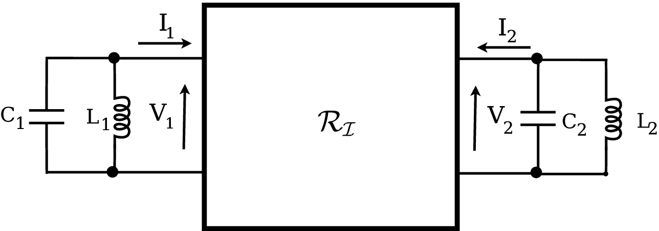
We go then to the synthesis of the network $\mathcal{R_{I}}$ that ends with a family $\mathcal{C}$, equivalent to the kaon system $\mathcal{K}^{\text{o}}$. We consider connected networks because they have a dual representation.

From Fig. 4 one has

Using now the standard relations between voltages and currents and performing a Laplace transformation one ends with

If $t=0$ is the initial time, $s=\sigma+\imath\omega$, F${}_{j}(s)$=C${}_{j}v_{j}(0)-\frac{1}{s}i_{\mathrm{L}_{j}}(0)$ includes the initial conditions. We call $\mathcal{Y}_{j}(s)$ the admittance function of the subnetwork $\mathcal{R}_{j}$, given by

Clearly, the frequency of each subnetwork, $\omega_{oj}$, is given by $\omega_{oj}=1/\sqrt{\mathrm{L}_{j}\mathrm{C}_{j}}$

On the other hand, the interaction network $\mathcal{R_{I}}$, initially without energy sources, is governed by (35), with $\mathbf{Y}:\mathbb{C}$ $\longmapsto$ $\mathbb{C}^{2\mathrm{x}2}$, that we write

with $y_{ij}(s)=\left.\mathrm{I}_{i}(s)/\mathrm{V}_{j}(s)\right|_{V_{k}=0}$; $j$ $\neq$ $k$, called the admittance parameters of the circuit.

Coming back to (40), it can be written as

with the matrices D$:=diag($C${}_{1}^{-1}$,C${}_{2}^{-1}$) and $\mathbf{\boldsymbol{\mho}}:=diag(\omega_{o1},\omega_{o2}$).

As was stated before, the states of the free network, $\mathbf{Y}(s)=\mathbf{0}$, are related to the unperturbed states of the quantum system, $\mathbf{\hat{H}}=\mathbf{\hat{H}}_{o}$. Consequently, the eigenfrequency of each subnetwork correspond to the neutral kaon masses $\omega_{oj}\longleftrightarrow m_{j}$, with $j$=$\mathrm{\scriptstyle K}^{\circ}$, $\mathrm{\bar{\scriptstyle K}}^{\circ}$. Then, CPT invariance implies $\omega_{oj}=\omega_{o}$ for all $j$ that forces

with $\mathbf{1}$ the identity $2\times 2$ matrix.

In order to obtain a linear differential equation of second order in time, one needs the initial conditions in F$(s)$. We consider zero port currents, $\mathbf{i}(0)=\mathbf{0}$. Notice that this initial condition is a necessary condition once one considers that $\mathcal{R_{I}}$ is initially without energy. Therefore can be used the usual methods of networks synthesis.

Then, from (39) to each node and (31) one has

that allows the term $\mathbf{D}\mathbf{F}(s)$ of (43) to be written as

Next we deal with the general form of the matrix Y$(s)$.

We are considering first reciprocal networks that implies that $y_{ij}(s)=y_{ji}(s),\forall s$. This is the case of any network composed by R, L and C [11]. Moreover, a connected reciprocal network of two ports reduces always to the so called structure $\boldsymbol{\Pi}$ (or its dual T) as is shown in Fig. 5

The topology $\boldsymbol{\Pi}$, implies a relationship between {Y_a,Y_b,Y_c} and the matrix Y [11]

We consider first the most simple case of a coupling between subnetworks defined by a matrix Y$(s)$ constant in $s$. This is the case of a matrix $\mathcal{R_{I}}$ of only resistors. Then

where {$\mathrm{G}_{a},\mathrm{G}_{b},\mathrm{G}_{c}$} are the conductances of $\mathcal{R_{I}}$.

The complete network results from the connection of a dipole to each port of $\mathcal{R_{I}}$ whose dynamics is given by

Here one can identify the matrices A and B of Eq. (4), i.e. A=DY, B=$\boldsymbol{\mho}^{2}$. Both matrices can be diagonalized under the same change of basis. The matrix DY is symmetric having two real positive eigenvalues. For this reason, the real part of the eigenvalues of K, that measure the time life of the decaying particles can be exactly fitted from Eq. (20).

Due to the fact that the quantum system of interest presents two different eigenvalues, the network we are looking for has to have a matrix B that besides being diagonalized by means of the same basis that the one for A, has different positive eigenvalues. This is achieved , in the case of an interaction circuit type $\boldsymbol{\Pi}$, varying their constitutive elements. Take for example a new matrix $\mathbf{\tilde{Y}}(s)$ with elements defined in terms of a resistor connected in parallel with an inductance, namely

with Y given in (47). Here the dependence on $s$ does the job

Now the following circuit equation results

where one can indentify B=$\boldsymbol{\mho}^{2}+\mathbf{DL}^{-1}$ whose eigenvalues are {$\omega_{o}^{2}+\frac{1}{C_{1}\mathrm{L}_{a}},\omega_{o}^{2}+\frac{1}{C_{2}\mathrm{L}_{b}}$} while A=DY. The network thus obtained is presented in Fig. 6

Now we are prepared to present the general $\mathcal{R_{I}}$ both connected and reciprocal that satisfies the requirement of equivalence. The admittance matrix is given by DY$(s)=\boldsymbol{\alpha}+\frac{1}{s}\boldsymbol{\beta}(s)$, while the matrix elements of Y$(s)$ are $y_{ij}=\alpha_{ij}+\frac{\beta_{ij}}{s}$, with $\alpha_{jj},\beta_{jj}$ positive and with the possibility that $\alpha_{ij},\beta_{ij}$ with $i\neq j$ can be negative.

We the take the inverse Laplace transform to (43) with initial condition $\dot{\mathbf{v}}(0)=\mathbf{0}$ to obtain the evolution equation

that completes the demonstration that one can get an evolution equation of the initial form (4). We can recognize that the matrix $\complement$ of (6) is defined in terms of the following:

Moreover, in terms of the circuit elements, one has

The conditions $\alpha_{11}=\alpha_{22}$ and $\beta_{11}=\beta_{22}$ ensures that [$\mathbf{A,B}$]=$0$ and in this case, the characteristic polynomial is trivially factorized. Consequently, as we have shown previously, the eigenvalues of $\complement$, from (20) and (21) are

plus their complex conjugates and with $\mathrm{A}_{j}$ and $\mathrm{B}_{j}$ eigenvalues of A and B respectively. As one should have $4\mathrm{B}_{j}>\mathrm{A}_{j}^{2}$, one can write a first order approximation for the eigenvalues as follows

By an appropriate choice of the circuit parameters that govern the eigenvalues {$\lambda_{j}$}, one can make them equal to those of the kaon matrix $\mathbf{K}=-(\mathbf{\Gamma+\imath M})$ and build up the $S$ matrix. In this way, the isomorphism between the electric networks $\mathcal{R}$ and the kaon system $\mathcal{K}^{\circ}$, is established.

The general interaction reciprocal network G-L equivalent, by $\boldsymbol{\Phi}_{S}$, to the kaon system is sketched in Fig. 7.

As it was stated before, there exists the alternative possibility of using the currents $i_{j}$ instead of voltages as generalized coordinates. The corresponding dual system (type R-C), presented in Fig. 8, is entirely equivalent to the kaon system as is the previous one.

References

- [1] J.L.Rosner, Tabletop time-reversal violation, Am.J.Phys.64 (8), 982-985, (1996)
- [2]
V. Alan Kosteleck, Ágnes Roberts, Analogue models for T and CPT violation un neutral-meson
oscillations, Phys. Review D 63, 096002-1 (2001) - [3] D.Cocolicchio, The Classical Analogue of CP-Violation, Foundations of Physics Letters 11 (1), 23-39, (1998)
- [4] R.P. Feynman, The Feynman Lectures on Physics, Volume 3 Quantum Mechanics, Pearson | Addison-Wesley, (1964)
- [5] M.W. Hirsch, S. Smale, Differential Equations, Dynamical System and Linear Algebra, Academic Press Inc, (1974)
- [6] V. I. Arnold, Ordinary Differential Equations, The MIT Press, (1995), 9th edition
- [7] T.D. Lee, Particle Physics and Introduction to Field Theory, Harwood Academic Publishers, (1981)
- [8] M. Antonelli, G. D’Ambrosio (Particle Data Group), CPT Invariance tests in neutral Kaon decay, Updated October (2009)
- [9] L. Wolfenstein, T.G. Trippe, C.-J. Lin (Particle Data Group), Tests of conservation laws, Updated June (2008)
- [10] C. Amsler et al. (Particle Data Group), PL B667, 1, (2008)
- [11] N. Balabanian, T.A. Bickart, S. Seshu, Electrical network theory, Wiley, (1969)
- [12] H. Carlin, A. Giordano, Network Theory: An Introduction to Reciprocal and Nonreciprocal Circuits, Prentice Hall, (1964)
- [13] B.D.H. Tellegen, The Gyrator, a new electric network element, Philips Res. Rept. 3, 81-101, (1948)
- [14] Marsden, Ratiu, Abraham, Manifolds, Tensor Analysis, and Applications, Springer T (2003)
- [15] Marsden, Ratiu, Introduction to Mechanics and Symmetry, Springer-Verlag (1994)
- [16] P.A.M.Dirac The principles of Quantum Mechanics, Oxford University Press, (1958), 4∘ edición
- [17] A.Galindo, P. Pascual Quantum Mechanics, Springer-Verlag, (1990)
- [18] J. R. Silvester Determinants of Block Matrices, Maths. Gazette 84, 460-467, (2000), http://www.mth.kcl.ac.uk/jrs/gazette/blocks.pdf
- [19] M. G. Caruso Isomorphism between the Schrdinger Dynamics and Classical Dynamics, Work of degree thesis
- [20] V.F. Weisskopf, E.P. Wigner, Z. Physik. 63 (54), 1930,65 (18), (1930)
- [21] C. D. Froggatt,H. B. Nielsen, Origin of Symmetries, World Scientific, (1991)
- [22] R.F. Streater, A.S. Wightman, PCT, Spin and Statistics, and all that, Princeton University Press, Third Edition (1980)
- [23] G. Lders, Proof of TCP Theorem, Ann. Phys. 2,1 (1957)
- [24] R.G. Sachs, The Physical of Time Reversal, The University of Chicago Press | Chicago and London, (1987)
- [25] T.D. Lee, R. Oehme, C.N. Yang, Remarks on Possible Noninvariance under Time Reversal and Charge Conjugation, Phys.Rev. 106 (2) 340-345, (1957)
- [26] J.H. Christenson, J.W. Cronin, V.L. Fitch, R. Turlay Evidence for the Decay of the K Meson, Phys. Rev. Lett. 13, 138, (1964)
- [27] J.J. Sakurai, Invariance Principles and Elementary Particles, Princeton University Press, (1964)
- [28] H.Whitney, Nonseparable and Planar Graphs, Trans. Amer. Math. Soc.,34 (1932), 339–362.
- [29] K. Hoffman, R. Kunze, Linear algebra, Prentice Hall Internacional, (1973)
- [30] H. Carlin, On the Physical Realizability of Linear Non-Reciprocal Networks, Prentice Hall, (1964)