The Nuclear Yukawa Model on a Lattice
Abstract
We present the results of the quantum field theory approach to nuclear Yukawa model obtained by standard lattice techniques. We have considered the simplest case of two identical fermions interacting via a scalar meson exchange. Calculations have been performed using Wilson fermions in the quenched approximation. We found the existence of a critical coupling constant above which the model cannot be numerically solved. The range of the accessible coupling constants is below the threshold value for producing two-body bound states. Two-body scattering lengths have been obtained and compared to the non relativistic results.
1 Introduction
The application of lattice techniques to nuclear physics is nowadays an active and fruitful field of investigation. This activity has been extensively developed in the last ten years and covers different aspects of the problem.
The first one aims to obtain relevant nuclear properties from ab-initio lattice QCD calculations (LQCD). In this approach, the elementary fields are quarks and gluons and all the numerical simulations depend on the very few QCD parameters: the bare coupling constant and the quark masses. The first task there is to generate the nucleon from its elementary constituents and thus this approach is necessarily limited to very light nuclei. First unquenched results on NN scattering length [1] and NN potentials [2, 3] have been obtained although still for large pion masses. Very recently, the binding energy of the A=3 and A=4 nuclei have been computed [4]. Although being performed in the quenched approximation, this is a result that seemed out of range just few years ago.
A second approach has been developed using the same techniques but in the framework of effective field theories, i.e. using nucleon and mesons as elementary fields. Lattice effective field theory (LEFT) has been first applied to study nuclear [5] and neutron matter [6] and was latter adapted to light nuclei [7]. The action describes non relativistic nucleons interacting via realistic, chiral inspired, NN potentials. These potentials depend on a large number of parameters depending on the order of chiral PT and have proved to be very successful in the non relativistic Faddeev-Yakubovski description of the A=2,3,4 nucleon problem. LEFT is a quantum mechanical description of a many body system, equivalent to a ladder potential models, that take the simplicity of the lattice techniques to go beyond few-body methods. At present this allows to treat bound states of nuclei up to A=12 nucleons and can be extended well beyond. A review on this approach can be found in [8].
Our aim in this work was to consider the simplest Quantum Field Theory (QFT) model of interacting fermions which was at the origin of nuclear forces: the Yukawa model. Since Yukawa pioneer work [9], the meson-exchange interactions constitute the starting point for building the NN potentials [10, 11, 12] which, inserted in Schrodinger-like equations, provides an ”ab-initio” description of light nuclei up to [13]. The potential approach, however, takes into account only a small, though infinite, fraction of diagrams of the perturbative series – the ladder sum. This represents a severe restriction of the interaction, specially taking into account the large values of the coupling constants involved. Chiral inspired NN models [14, 15, 16], which can be formally distinguished from the traditional meson-exchange ones, suffer from the same restrictions.
To incorporate the full content of the meson-exchange Lagrangian we have used the standard lattice techniques [17], developed in the context of QCD. They are based on a discrete Feynman path integral formulation of QFT and provide nowadays a genuine way to solve non perturbatively such problems. Preliminary results of this work can be found in [18, 21, 22]. A similar study was undertaken in [23] in the frame of a purely scalar model.
A few lattice investigations of the Yukawa model with an additional term have also been performed some time ago in the spontaneously broken phase [24]. Similar models were studied in the past (see for instance [17] and references therein). and the existence of numerical instabilities beyond a critical value of the coupling were found. Different schemes were used for the discretization of the meson field, obtaining critical values of the lattice coupling slightly different, but corresponding to the same continuum limit. More recently the phase structure of a chirally invariant lattice Higgs-Yukawa model was studied to establish Higgs boson mass bounds [25, 26]. None of these studies was however interested to investigate the existence of two-fermion bound states in the original Yukawa model.
The plan of the paper is as follows. In section 2 we describe the model and its discretization as well as the approximations in use. Section 3 contains the detail of the Monte Carlo simulations and the results for the renormalized fermion mass. The two-body binding energies and scattering lengths are presented in section 4 and compared to the non relativistic results. Some concluding remarks are finally drawn in section 5.
2 The model
We have considered the simplest renormalizable Quantum Field Theory describing a fermion () – meson () interaction. It is given by the Lagrangian density:
| (1) |
with, in Euclidean space,
| (2) | |||||
| (3) | |||||
| (4) |
The fermion field is supposed to describe a nucleon (N) and the meson field a – more or less fictitious – scalar particle () responsible for the attractive part of the NN potentials. The Lagrangian depends on four parameters: the fermion and meson masses and two dimensionless coupling constants and . The Yukawa coupling in Eq. (4) admits several possibilities depending on the choice of the matrix: for the scalar case and for the pseudo-scalar one. In this work we will restrict to the scalar coupling, for it is known to produce a stronger fermion-fermion attraction.
This theory can be treated perturbatively by computing order by order the contributions in , as is done for example in QED for computing the anomalous magnetic moment of the electron. Bound states nevertheless appear only non-perturbatively, when contributions at all orders in the coupling are taken into account.
Non-perturbative tools are extensively used in the context of QCD. Among them, the lattice techniques provide a reliable numerical method for solving any QFT on a discretized Euclidean space-time. A very basic description of these techniques is given below. The interested reader can found a detailed explanation in e.g. [17].
The vacuum expectation values of the operators involved are obtained in the Path Integral approach which consist in computing integrals like:
| (5) |
where the Euclidean action plays the role of a probability distribution in a Monte Carlo simulation.
The discretized Euclidean action can be written, according to Eq. (1), in the form:
where is the lattice spacing and denotes a point with coordinates () and . In practice we have taken equal spatial dimensions and a temporal one with .
For the free Dirac action , we have used Wilson fermions. They consist in adding to the, naively discretized, derivative term of the Dirac Lagrangian (2) a Laplacian operator in order to remove the spurious poles at the boundaries of the Brillouin zone [17]. The free Dirac action is then written as a bilinear form in the dimensionless fermion fields :
| (6) |
where
| (7) |
is the Dirac-Wilson operator, and
| (8) |
is the hopping parameter.
In terms of the dimensionless meson field , the discrete Klein-Gordon action reads:
| (9) |
The interaction term takes the form
| (10) |
where is the lattice Yukawa coupling.
Taking together the fermion (6), meson (9) and interaction (10) terms, the lattice Euclidean action can be written in the form:
| (11) |
where includes both the Klein-Gordon and the term
| (12) |
and the fermionic part is written in terms of the interacting Dirac operator
| (13) |
Notice that the model is now made dimensionless. When needed, the physical quantities – masses, energies, etc. – will be given in terms of the lattice spacing.
One of the most demanding issues when computing the vacuum expectation values (5) comes from the Grassmannian character of fermion fields, that have to be integrated out by algebraic methods. For example the fermion propagator, corresponding to ,
| (14) |
implies the evaluation of a determinant and inverse of an operator that, even for moderate lattices, , has a dimension of . Moreover, if a Monte Carlo simulation is to be done using Eq. (14), the probability distribution for meson configurations is given by , what means evaluating a large determinant in every Monte Carlo step . This can be avoided by the use of Hybrid Monte Carlo techniques that nevertheless are the main source of time spent in the simulation. This task is considerably simplified in the “quenched” approximation that, from the computational point of view consists in setting independent of the meson field in the fermionic integral.
From a physical point of view, the quenched approximation avoids the possibility for a meson to create a virtual nucleon-antinucleon pair (see figure 1). Due to the heaviness of the nucleon with respect to the exchanged meson this approximation is fully justified in low energy nuclear physics and implicitly assumed in all the potential models.

We have furthermore chosen in our simulation to neglect the meson self-interaction term setting in (12). This choice is consistent only in the quenched approximation. In a full QFT treatment of this model, the fermions loops will generate meson self-interactions, that require a counter-term for renormalizability.
The model depends on three dimensionless parameters , , and usually set via the hopping parameter (8). These parameters appearing in the Lagrangian are not physical: they are modified by the interaction so that they have to be renormalized. Our first task to map the bare quantities into the renormalized parameter space
In the quenched approximation and for , mesons do not interact each other and therefore its mass renormalize trivially . In the following we will omit subscripts and denote the dimensionless meson mass by . The lattice spacing does never appear explicitly and it has to be fixed by setting a physical dimensional quantity. We do that by identifying the unchanged meson mass to a physical meson of GeV, a typical value used in the NN models. If we are using in our simulations , the lattice spacing is given by .
Coupling constant renormalization is a more involved issue. Renormalized coupling constants were computed in a previous work [18]. For the scalar coupling no sizable effect of renomalization was found, i.e. in a wide range of momenta. From now on, we will denote by this unique coupling constant.
The remaining task for finding the adequate parameter space is thus to compute the renormalized fermion mass as a function of the bare parameters. This will be described in the next section.
3 Monte-Carlo simulation
3.1 Generating field configuration
In the above defined conditions, the generation of meson field configurations is straightforward. This can be seen by writing the Klein-Gordon action (9) in Fourier space
| (15) |
where denotes the Fourier transform of the meson field
and we have introduced the quantity
which depends on the lattice discretized momenta
One can see from equation (15) that the different Fourier modes of the meson field appearing in the action are decoupled and can be generated independently.
The Monte Carlo algorithm becomes then trivial as it is enough to produce at each lattice point , independent complex scalar fields with a probability density given by
| (16) |
i.e. centered Gaussian distributions, both for their real and imaginary parts, with a variance depending on and the constraint imposed by the reality of . This method generates configurations that are statistically independent, thus saving a large amount of computing time with respect to the Metropolis algorithm.
The scalar fields in configuration space are finally obtained by performing an inverse Fourier transform on . It follows from the particular form (16) that are also centered Gaussian with a width , independent of , given by
| (17) |
Note however that the are now correlated. The correlation function is given by
| (18) |
which is the scalar propagator in configuration space. It is interesting to note that the parameter in Eq. (17) is related to the lattice regularization of the potential at the origin,
| (19) |
The -dependence of is displayed in figure 3 for different values of the lattice size, . It behaves like in the two trivial limits and with a plateau in between, which is the region we are interested in. The parameter allows a discussion of the discretization and finite volume errors in terms of physically well defined limiting cases:


The non-relativistic Yukawa potential can be computed for the discrete lattice using Eq. (18) but summing only over spatial directions. The resulting potential () for and is represented in figure 3 (Black dots) and compared to the continuum result (Solid line). The main effect of discretization is the regularization at the origin and is seen to be negligible beyond the very first points. This potential will be used in section 4 to compare continuum and lattice results.
The appearance of volume effects depend crucially on the value: they are very small for large values of but important when . As a matter of fact for a given value of , there is a minimal lattice size below which the lattice artifacts are dominant. We took this constraint into account in the present work.
3.2 Zero modes of Wilson-Dirac Operator
When computing physical observables, the integration over the fermionic fields is performed analytically and the result is expressed in terms of the inverse Dirac operator (13). This has been explicitly done in eq. (14) for the fermion propagator which constitutes the building block of the lattice simulations. When working in the quenched approximation, one can set and the relevant numerical task is thus reduced to compute for an statistical ensemble of meson field configurations.
| (20) |
Due to translational invariance one is left in practice to compute , that is to solve the linear system:
| (21) |
It is worth noticing that in the full QFT formulation every configuration is weighted by the determinant of the Dirac operator and therefore the configurations yielding an ill-conditioned linear system (21), i.e with , do not contribute to the functional integral. In the quenched approximation, however, this is no longer true and “ill-conditioned configurations” can be sampled.
As a practical measure of the “ill-conditioness” of we have considered its “condition number” defined as the ratio between the largest to the lowest eigenvalue modulus[19]. The largest is this number the more difficult is to solve the linear system. Depending on the method used for that purpose, either the algorithm cannot find the solution, or the round-off errors make the solution wrong. In exact arithmetic the condition number measures how the solution changes when the second member of linear system slightly changes.
We have found that such “ill-conditioned configurations” appear in the Yukawa model for almost any when . In this case the inversion of the Dirac operator becomes in practice impossible [20]. For illustrative purposes, we have plotted in figure 4 the condition number of as a function of the lattice coupling constant for an ensemble of configurations at fixed value of . As one can see, the condition number of a given configuration diverges on a discrete set of values for indicating the practical impossibility to compute the nucleon propagator. The precise values where this divergence occurs depend on the particular configuration, on the values of and and on the lattice size. It turns out however that the situation described in figure 4 is generic for the quenched Yukawa model.

The existence of zero modes in the quenched Yukawa model was already found in [27] but the numerical results performed with very small lattice let these authors suspect the existence of a second allowed region at large values of . It can be shown however that this result is a volume artifact as the second region disappears exponentially with the number of lattice sites in the thermodynamical limit. This issue as well as some properties of the interacting Dirac operator (13), in particular the fact that its spectral properties do not depend independently of and but rather on their ratio, will be treated in detail in a forthcoming publication [20].
As a conclusion, the numerical simulations in the quenched Yukawa model are limited to values of the lattice coupling constant . Using a typical value of , this corresponds to , that is which is of the same order than the in the nonperturbative region.
3.3 Renormalized Fermion mass
Renormalized particle masses are obtained in Lattice QFT by considering the time evolution of the correlator matrix defined as:
| (22) |
where creates a particle state at the origin and destroys it at . The tensorial indexes – depending on the type of particle – are implicit and the vacuum expectation value is obtained through an average over field configurations. It can be shown that the correlator matrix (22) has contributions from all the particle states satisfying , and has the form
| (23) |
For , it behaves as a sum of hyperbolic cosine with the rest mass of the particle states:
| (24) |
Using the above equation at two consecutive times one can extract an effective mass
| (25) |
which, at large enough euclidean times, will display a plateau region that will be identified to value.
In the case of one fermion state (), the correlator matrix is he matrix:
| (26) |
where is the propagator defined in Eq. 14. The case of two fermion states will be discussed in section 4.
The fermion masses extracted in this way are presented in figure 6 for , a lattice size and several values of the lattice coupling ranging from to . In the free case, this mass is already different from the bare one due to lattice artifacts and it is given by:
| (27) |
with and . This expression is used to fit the interacting masses in terms of two parameters and . The result of this parametrization is indicated by full lines in figure 6. Note that at the renormalized fermion mass vanishes. As one can see, renormalized masses are smaller with growing values of the scalar coupling constant, or in other terms, . This indicates that the renormalized nucleon mass is made lighter by a scalar coupling.
The fitted coefficient is presented in figure 6. This coefficient can be calculated in lattice perturbation theory which provides a test of numerical simulations. It is quadratic in the coupling constant
| (28) |
with coefficient depending on the scalar mass and on the lattice size .


The region of parameter space to perform the numerical simulations of physical interest is limited by the constraint which corresponds to . In order to avoid large lattice artifacts the condition must hold, what restricts the useful parameter space to a narrow band in the vicinity of with the constraint indicated in the preceding section, say .
4 Two-fermion states
Our main interest in this work is to study the interactions between fermions and thus the properties of the two-body states. In this respect, our reference will be the results provided by potential models in the non relativistic ladder approximations. These are summarized in what follows.
4.1 Non relativistic results
Let us first consider the non relativistic system of two particles with equal mass , interacting by a Yukawa potential of strength and range parameter
The binding energy () and scattering length () are given by
| (29) | |||||
| (30) |
where and are respectively the binding energy and scattering length of the dimensionless S-wave Schrodinger equation.
| (31) |
with a coupling constant related to the original parameters () by
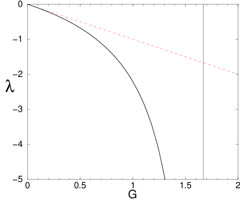
The functions and are displayed in figures 8 and 8. The convention used for the scattering length corresponds to . The critical value for the appearance of the ground state is . At this value has a pole and it can be shown that for small values of G one has
| (32) |
which corresponds to the Born approximation.

4.2 Binding energies
We will restrict ourselves to study the system of two identical fermions, say , in the state. The general form of the interpolating field for a two fermion state reads
| (33) |
where depends on the quantum number of the state. For a state one has . In the matrix form (33) can be written as
Using the interpolating field (33), the correlator becomes
where denotes the fermion propagator.
In order to decrease the contribution of the excited states we have introduced a smearing procedure. This consists in modifying the interpolating field in the following way:
| (34) |
where is some smearing function to account for the spatial extension of the state. As we are interested in the s-wave, the smearing can be done over the whole timeslice in an efficient and inexpensive way by choosing the smearing function to be a constant, . After performing the appropriate Wick contractions, the time-correlator results:
| (35) |
where the 4x4 matrices and are respectively:
| (36) | |||||
| (37) |
and is the solution of the linear system
| (38) |
This three-dimensional smearing efficiently removes higher energy contributions to the correlator as it can be seen in figure 10 where the effective mass (25) is plotted both for the local and smeared interpolating fields. It can be seen that for large values the effective mass tends to a plateau which actually defines the mass of the state. If the local sources were used we would have needed larger values of to be able to find a plateau in the masses.
An interesting property of this smearing is that the two-body free correlator is the square of the one-body one at any value of , i.e., the effective mass of the two-body state is rigorously constant and exactly twice that of one particle.


The binding energy of a two-fermion state with total mass is defined as where denotes the mass of the fermion. In figure 10 we show this binding energy as a function of the lattice size for a given set of parameters. The dotted line is a fit obtained with a dependence. As it can be seen in this figure, the binding tends to zero in the infinite volume limit. This indicates that this two-fermion system has no bound state for this particular set of parameters. The situation is however the same for the whole range of parameters accessible in the numerical simulations. Although assuming that this pathology could be associated to the quenched approximation it is physically surprising that no any NN bound state could be generated unless the NN̄ pairs creation (unquenched Yukawa model) are taken into account.


4.3 Scattering lengths
Since there is no bound state below the critical coupling constant, we can only access to the scattering properties of the state. The scattering observables cannot be obtained in Euclidean time in the infinite volume limit [28] but can be extracted from the volume dependent binding energy measured on finite lattices, like for instance the one plotted in figure 10. The underlying formalism was developed by Luscher in [29, 30] who gave a expansion of the the binding energy . In its leading order it reads:
| (39) |
Taking the binding energy values of figure 10 and equation (39), the NN scattering lengths have been extracted. The results corresponding to , , and are displayed in fig 12. They manifest a constant behavior of as a function of the lattice size L, indicating that the first order expression we used to extract the scattering length is justified. The dimensionless coupling constant of the nonrelativistc model for the parameters of figure 12 is . The corresponding non relativistic scattering length value, given by figure 8, is (solid line), quite close to its Born approximation (dashed line).
This study has been performed for several values of . The dependence of on the coupling constant is plotted in figure 12, for a lattice size of (, ). One can see that the lattice results notably departs from the non relativisitc ones (solid line) and are above the Born approximation (dashed line). In figure 12 the NR scattering length has been computed using the lattice discretized potential of figure 3. As one can see, the regularization of the potential at the origin has no effect in the scattering length (indistinguishable from the continuum result in the figure). This is due to the fact that the scattering length is a zero energy observable and therefore is not very sensitive to the details of the interaction. From the preceding analysis we conclude that the repulsive effect shown by the lattice data is not related to the lattice potential discretization at short distances.
The values of the accessible coupling constants extend beyond the Born regime but are still far from the pole behavior corresponding to the appearance of the first bound state displayed in figure 8. The difference between the lattice and NR results may indicate strong repulsive corrections. These kind of corrections are already manifested in the bound state problem when solving the same Yukawa model both in Light Front [31] and Bethe-Salpeter [32] ladder equations.
5 Conclusion
We have considered the quantum field theory solution of the simplest nuclear Yukawa model consisting on two identical nucleons interacting via a scalar meson exchange. The choice of the scalar coupling with respect to pseudo scalar one was taken in order to optimize the appearance of two-body bound states we were interested in.
The problem has been solved using the standard lattice techniques, based on the path integral formulation of the theory on a discretized space-time. The meson field has been described by a discretized Klein-Gordon Lagrangian without self-interacting term and the Dirac-Wilson discretization was chosen for the fermion.
The resulting model is fully relativistic and was solved by neglecting only the NN̄ loops generated from the meson field in the so called quenched approximation. This simplification is physically justified by the heaviness of the nucleon and is anyway implicit in all nuclear models.
The numerical simulations were performed along the physical line where and denote respectively the meson and nucleon renormalized masses. The solutions were found only for coupling constants below some critical value . Above this value the ubiquitous presence of fermion zero modes made the problem numerically unsolvable. The addition of a pseudo scalar coupling term does not make the problem simpler. The present situation does not allow to judge whether this problem is related to the particular fermion discretization used. However the same problem was described in the past to affect naive fermions [24]. This seems to indicate that the use of Wilson fermions is not responsible for the problem.
The range of the accessible coupling constants is below the threshold value for producing two-body bound states, which in the non relativistic potential approximation turns to be and in the Bethe-Salpeter one sensibly larger. In the accessible region of the NN scattering length was calculated using the Luscher procedure. The values found were in agreement with the non relativistic models for low coupling constants but show strong repulsive effects when increasing .
We conclude that the quenched approximation of the Yukawa model (scalar coupling) is not able to produce two-nucleon bound states. Although this pathology is manifested in the quenched approximation it suggests that the non-relativistic results based on one-boson exchange potentials have no direct counterpart in the quantum field theory approach.
Acknowledgment
The authors are pleased to acknowledge the fruitful discussions held at LPT with Ph. Boucaud, J.P. Leroy and O. Pene who fully participated in the early stages of this work. We thank the staff of the Centre de Calcul IN2P3 in Lyon where some of the numerical calculations were performed. This works has benefit from the French-Spanish Collaboration Agreement IN2P3- MICINN.
References
- [1] S.R. Beane, P.F.Bedaque,K. Orginos, M.J. Savage, Phys. Rev. Lett. 97 (2006) 012001, hep-lat/0602010
- [2] N. Ishii, S. Aoki and T. Hatsuda, Phys. Rev. Lett. 99, 022001 (2007).
- [3] Noriyoshi Ishii, PoS LAT2009:019,2009.
- [4] T. Yamazaki, Y. Kuramashi, A. Ukawa, Phys. Rev. D81:111504,2010. , arXiv:0912.1383 [hep-lat]
- [5] H.M. Muller, S.E. Koonin , R. Seki, U. van Kolck, Phys. Rev. C61, 044320 (2000).
- [6] D. Lee, B. Borasoy, Th Schaefer, Phys. Rev. C 70, 014007 (2004)
- [7] E. Epelbaum, H. Krebs, D. Lee, U. Meissner, Eur. Phys. J. A45, 335-352, 2010.
- [8] D. Lee, Prog. Part. Nucl. Phys. 63, 117 (2009), arXiv:0804.3501 [nucl-th].
- [9] Yukawa, Proc. Math. Soc. Jap 17 (1935) 48
- [10] V.G. Stoks et al, Phys. Rev. C49 (1994) 2950
- [11] R.B. Wiringa et al, Phys. Rev. C51 (1995) 38
- [12] R. Machleidt, Phys. Rev. C63 (2001) 0240041
- [13] H. Kamada et al, Phys. Rev. C64 (2001) 044001, S. Pieper, Nucl. Phys. A751 (2005) 516
- [14] S. Weinberg, Nucl. Phys. B363 (1991) 3
- [15] C. Ordonez et al, Phys. Rev. C 53 (1996) 2086
- [16] E. Epelbaum, W. Glockle, U.G. Meissner, Nucl. Phys. A671 (2000) 295.
- [17] I. Montvay and G. Munster, Quantum Fields on a Lattice, Cambridge Univ. Press (1994)
- [18] F. de Soto, J. Carbonell, C. Roiesnel, Ph. Boucaud, J.P. Leroy, O. Pene, Nucl. Phys. B Proc. Suppl. 164 (2007) 252.
- [19] Y. Saad Iterative method for sparse linear systemManchester University Press (2000).
- [20] J.Ch. Anglès d’Auriac F. de Soto in Preparation.
- [21] F. de Soto, J. Carbonell, C. Roiesnel, Ph. Boucaud, J.P. Leroy, O. Pene, Eur. Phys. J A31, 777 (2007); hep-lat/0610084
- [22] F. de Soto, J. Carbonell, C. Roiesnel, Ph. Boucaud, J.P. Leroy, O. Pene, Nucl. Phys. A 790 (2007) 410 ; hep-lat/0610086
- [23] T. Nieuwenhuis, J.A. Tjon, Phys. Rev. Lett. 77 (1996) 814
- [24] J. Polonyi, J. Shigemitsu, Phys.Rev. D38 (1988) 3231; I. Lee, J. Shigemitsu and R.E. Shrock, Nucl. Phys. B330 (1990) 225; I. Lee, J. Shigemitsu and R.E. Shrock, Nucl. Phys. B334 (1990) 265.
- [25] P. Gerhold, K, Jansen, JHEP 0710:001,2007 , hep-lat 0707.3849
- [26] P. Gerhold, K. Jansen, JHEP 1004:094,2010, [hep-lat] 1002.4336
- [27] W. Bock, A.K. De, K. Jansen, J. Ijersak, Th. Neuhaus and J. Smit, Nuc. Phys. B344 (1990) 207Ñ237
- [28] L. Maiani, M. Testa, Phys. Lett. B245 (1990) 585
- [29] M. Luscher, Commun. Math. Phys. 104 (1986) 177
- [30] M. Luscher, Commun. Math. Phys. 105 (1986) 153
- [31] M. Mangin-Brinet, J. Carbonell, V. Karmanov, Phys. Rev. C68 (2003) 055203
- [32] J. Carbonell, V. Karmanov, Eur. Phys. J. A32 (2010), 387–397.