The muon $g-2$ is a precisely measured quantity, and hence it is an excellent probe of new physics at the TeV scale. The measurement at BNL was finalized in 2006 [7]. After including a small shift in the value of the proton-to-muon magnetic ratio reported since then [58], the experimental value is [13]:

As for the SM prediction, the recent improvement in the low-energy $e^{+}e^{-}\to$ hadrons data from BaBar [59], BES [6], CMD-2 [60], KLOE [61, 62] and SND [63] allows us to reduce the uncertainty. In Ref. [8], the SM prediction has been evaluated as (after correcting a typo in Ref. [8]),

which includes all the major updates on the $e^{+}e^{-}\to$ hadrons data, and adopts the estimate [64], $a_{\mu}^{\rm l{\mbox{-}}by{\mbox{-}}l}=10.5(2.6)\times 10^{-10},$ for the light-by-light contribution. Other independent analyses [9, 10, 11] based on the $e^{+}e^{-}$ data give similar estimates. Hence, the observed value of the muon $g-2$ is larger than the SM prediction by

which differs from zero by 3.2 $\sigma$. It is tempting to interpret the difference as a contribution of new particles with the muon quantum number, such as smuons in the SUSY SM. Throughout this article we assume that the MSSM contribution accounts for this discrepancy.

In the MSSM, the contribution to the muon $g-2$ has been calculated up to and including the two-loop level [65]. In view of the smallness of the two-loop contribution, in this paper we restrict our analyses in the one-loop approximation¹¹ 1 The effect from the $\tan\beta$-enhanced resummation in the muon-muon-Higgs vertex can change the MSSM contribution by about 10% [66], which does not affect the conclusions in the present paper significantly..

At one-loop, the MSSM contribution comes from the chargino contribution $a_{\mu}(\widetilde{\chi}^{-})$ and the neutralino contribution $a_{\mu}(\widetilde{\chi}^{0})$. The relevant one-loop expressions in the notation of Ref. [1] are found e.g. in Refs. [67, 68], as:

where

Even though these expressions are useful for numerical calculations, they are not particularly illuminating for the purpose of understanding their dependences on the SUSY parameters. The main disadvantage of the above expressions is that they are written in terms of the mass eigenstates, in terms of which the dependences on the SUSY breaking parameters are hidden by the electroweak symmetry breaking that causes complex mixings.

In the weak eigenstates, the structure of the one-loop contributions becomes much more transparent. This simplification occurs since the expressions in the weak eigenstates are equivalent to the $m_{Z}/m_{\rm SUSY}$ expansion, where $m_{\rm SUSY}$ is the typical SUSY breaking mass scale. The price we have to pay is that the leading terms in the expansion are not useful when $m_{\rm SUSY}\sim m_{Z}$. However, we will find below that this expansion is very useful when analyzing the SUSY parameter dependence.

The leading terms in the $m_{Z}/m_{\rm SUSY}$ expansion are given by the five diagrams (a) to (e) in Fig. 1, whose contributions can be expressed compactly as

respectively. The functions $F_{a}(x,y)$ and $F_{b}(x,y)$ are defined as:

which are symmetric under exchange of the two arguments.

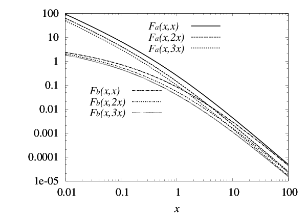
The functions $G_{3}(x)$ and $G_{4}(x)$ are monotonically decreasing for $0<x<\infty$, and hence the functions $F_{a}(x,y)$ and $F_{b}(x,y)$ are positive for all positive $x$ and $y$. In Fig. 2, we show the behaviors of $F_{a,b}(x,nx)=F_{a,b}(nx,x)$ for $n=1,\ldots,3$.

The expressions (6a)-(6e) allow us to make a few general observations on the SUSY parameter dependences. The first one is that the contributions from the diagrams (a)-(c) in Fig. 1 are positive, while those from the diagrams (d) and (e) are negative for $M_{2}\mu$ and $M_{1}\mu>0$. In addition, if the mass-splitting in the $(\tilde{\nu}_{\mu},\tilde{\mu}_{L})$ doublet is small we can conclude that the sum of the diagrams (a) and (d), or that of Eqs. (6a) and (6d) is always positive, because $F_{a}(x,y)$ is always larger than $F_{b}(x,y)$ for the same arguments as shown in Fig. 2. If the contributions from the diagrams (b), (c), and (e) are suppressed, being proportional to $g_{Y}^{2}=g^{2}\tan^{2}\theta_{W}$, we can conclude that $M_{2}\mu$ should be positive in order to explain the positive deviation of the muon $g-2$ from the SM prediction in Eq. (3).

In fact, the only way to obtain a positive MSSM contribution for $M_{1}\mu<0$ and $M_{2}\mu<0$ is to make the contribution from the diagram (e), Eq. (6e), dominates over the others, which requires $(M_{2}/m_{\tilde{L}}^{4})F_{a}(M_{2}^{2}/m^{2}_{\tilde{L}},\mu^{2}/m^{2}_{\tilde{L}})\ll\tan^{2}\theta_{W}(M_{1}/m_{\tilde{E}}^{4})F_{b}(M_{1}^{2}/m^{2}_{\tilde{E}},\mu^{2}/m^{2}_{\tilde{E}})$. This situation is realized for $|M_{1}|,m_{\tilde{E}}\ll|M_{2}|,m_{\tilde{L}}$: for instance, when $(\tan\beta,\mu,m_{\tilde{E}},m_{\tilde{L}},M_{2},M_{1})=(50,-300,120,1200,1000,100)$, where the mass dimension is counted in units of GeV, the diagram (e) dominates over the others, and the predicted value of $a_{\mu}$ is within the 1-$\sigma$ favored region. In this example, an $M_{1}\mu<0$ solution is realized by setting $M_{2}/M_{1}=m_{\tilde{L}}/m_{\tilde{E}}=10$. We find that all the solutions with $M_{1}\mu<0$ require both $|M_{2}/M_{1}|\gg 1$ and $m_{\tilde{L}}/m_{\tilde{E}}\gg 1$. However, as discussed later, scenarios with heavy left-handed sleptons do not lead to a significant signal in the electroweak precision measurements, and we do not consider such scenarios hereafter.

Another interesting observation is that in the case where $\mu$ is large as compared to the SUSY breaking soft mass parameters, the contributions from the diagrams (a) and (c)-(e) are suppressed by $1/\mu$, as manifestly shown by the Higgsino propagator in the diagrams Figs. 1 (a) and (c)-(e). On the other hand, the diagram (b) is proportional to $\mu$, which makes this contribution important.

The above observations can be made explicit by neglecting the D-term and the F-term contributions to the slepton mass matrices, which makes $m_{\tilde{\mu}_{L}}=m_{\tilde{\nu}}=m_{\tilde{L}}$ and $m_{\tilde{\mu}_{R}}=m_{\tilde{E}}$, where $m_{\tilde{L}}$ and $m_{\tilde{E}}$ are the left-handed and the right-handed slepton soft SUSY breaking masses, respectively. Then, Eqs. (6a)-(6e) simplify as

where

Only for the above specific scenario with $m_{\tilde{L}}/m_{\tilde{E}}\gg 1$ and $|M_{2}/M_{1}|\gg 1$, Eq. (8e) dominates over the others and $M_{1}\mu<0$ is required to account for the positive shift, Eq. (3). In the very heavy Higgsino case with $|\mu/M_{1}|,|\mu/M_{2}|\gg 1$, Eq. (8b) dominates, and $M_{1}\mu>0$ is necessary to account for the positive shift. Except for the above two cases, Eq. (8a) dominates, and $M_{2}\mu>0$ follows.

We note that the above discussion on the favored signs of $M_{1}\mu$ and $M_{2}\mu$ are valid equally for both positive and negative $M_{1}$ and $M_{2}$ since the signs of $M_{1}$ and $M_{2}$ enter only through the combinations $M_{1}\mu$ and $M_{2}\mu$. In particular, we can use the same argument to identify the favored signs of $M_{1}\mu$ and $M_{2}\mu$ also for a model with ${\rm sgn}(M_{1})=-{\rm sgn}(M_{2})$, which is realized in some parameter regions of the mixed moduli and anomaly mediation model [69].

A comment on the SUSY breaking tri-linear coupling $A_{\mu}$ is in order here. In the one-loop order, the parameter $A_{\mu}$ enters only through the $\tilde{\mu}_{L}$-$\tilde{\mu}_{R}$ mixing in the combination $(A_{\mu}^{*}-\mu\tan\beta)$ in the diagram Fig. 1 (b). In order for $A_{\mu}$ to affect the muon $g-2$ significantly, Fig. 1 (b) should dominate over the others, but it implies large $|\mu|$ according to the above discussions. Since there is no attractive SUSY breaking scenarios that lead to a huge magnitude of $|A_{\mu}|\sim|\mu|\tan\beta$, and since moderate values of $|A_{\mu}|\mathop{}_{\textstyle\sim}^{\textstyle<}|\mu|$ do not affect the qualitative behavior, we set $A_{\mu}=0$ in the following, unless otherwise stated²² 2 For the possibility of explaining the muon $g-2$ anomaly using a large $A$ term, see e.g. Ref. [70]..

In Fig. 3 we show contour plots of the SUSY contribution to the muon $g-2$ as a function of the right-handed slepton mass $m_{\tilde{E}}$ and the $SU(2)_{L}$ gaugino mass $M_{2}$. In the figures, we examine the four combinations of $\tan\beta$ and $\mu$; $\tan\beta=10$ or 50 and $\mu=200$ or 800 GeV. As for the other relevant SUSY parameters, we assume the gaugino mass unification condition, $M_{1}/M_{2}=(5/3)\tan^{2}\theta_{W}$, and the left-handed slepton mass is taken to be equal to the right-handed slepton mass, for simplicity. Under these assumptions, we plot, from the lower left corner, the $+3\sigma$, $+2\sigma$, $+1\sigma$, $-1\sigma$ and $-2\sigma$ contours. (We do not plot $-3\sigma$ curves since those lie outside of the panel for Fig. 3(a), (b), (c) and (d)). The area surrounded by the $\pm 1\sigma$ contours is shaded. The vertical dotted lines give the lower bound on $M_{2}$ beyond which the lightest chargino mass becomes less than the experimental limit, 103.5 GeV [71]. Also shown by the horizontal dotted lines are the stau mass limit, 81.9 GeV [13]. We also show the contour of a constant “electroweak $\chi^{2}$ factor”, defined as the squared sum of the SUSY contributions to the electroweak $S_{Z}$- and $T_{Z}$-parameters [1] and to $m_{W}$;

The parameter regions in the left-bottom side of the dash-dotted curves give $\Delta\chi^{2}_{\rm EW}>0.5$, and there can be a hint of SUSY contributions to the electroweak observables in the near future³³ 3 The “dips” in Figs. 3 (a) and (c) at $M_{2}\simeq 120$GeV and 350 GeV $\mathop{}_{\textstyle\sim}^{\textstyle<}m_{\tilde{E}}\mathop{}_{\textstyle\sim}^{\textstyle<}400$ GeV happen since around this region there is a destructive interference between the combination “$\Delta T-\Delta\overline{\delta}_{G}/\alpha$” and the $\Delta R_{Z}$ term in $\Delta T_{Z}$ (see eq. (16b)), which makes the contribution from $\Delta T_{Z}$ to $\Delta\chi_{\rm EW}^{2}$ small.. See discussions in Section 4 for details.

In the figures, the sample points MSSM1–MSSM6 denoted by the cross symbols ($\times$), are chosen in the 1-$\sigma$ allowed region of the muon $g-2$ where $\Delta\chi^{2}_{\rm EW}>0.5$. They represent the two extreme cases where either a slepton (2,4,6) or an ino (1,3,5) is light. Our choices of $\mu$ and $M_{2}$ allow us to cover the cases where the lighter chargino is wino-like (3,4,5), Higgsino-like (2), or mixed (1,6). We use these six MSSM sample points in the study of the electroweak observables in later sections. The choice that there is either a light ino or a light slepton is interesting in view of the electroweak study since if there is a light new particle with nonzero electroweak quantum numbers, the contribution to the $S_{Z}$- and $T_{Z}$-parameters [1] and to $m_{W}$ can be significant.

For these sample points, we present separate contributions from individual diagrams and their sum in Table 1. In the table, we show the sum of the five terms in the column ‘(a)-(e)’, and the total SUSY contribution obtained without using the $m_{Z}/m_{\rm SUSY}$ expansion in the column under ‘total’. By comparing these two columns, we confirm for all the six cases that the leading terms in the $m_{Z}/m_{\rm SUSY}$ expansion give an excellent approximation. The last column shows the pull factor

where the mean $\langle\delta a_{\mu}\rangle$ and the error $\Delta\delta a_{\mu}$ are taken from Eq. (3).

For $\tan\beta=10$ and $\mu=200$ GeV shown in Fig. 3(a), the 1-$\sigma$ allowed region is very roughly given by $550{\rm GeV}\mathop{}_{\textstyle\sim}^{\textstyle<}1.7m_{\tilde{E}}+M_{2}\mathop{}_{\textstyle\sim}^{\textstyle<}800$ GeV. Here, the diagram (a) gives the dominant contribution, as can be read off from the rows 1 and 2 in Table 1, respectively, for the MSSM points 1 and 2.

For a larger $\mu$ like $\mu=800$ GeV shown in Fig. 3(b), the allowed region becomes narrower, partly due to the heavier Higgsinos, and partly because of the constraint from the stau mass lower bound $m_{\tilde{\tau}}>81.9$ GeV [13]. In the parameter region of Fig. 3(b), the diagram (b) becomes more important because all the other diagrams are suppressed by the heavy Higgsino mass, as discussed above. This can be explicitly verified from Table 1, in the rows 3 and 4. In the MSSM point 3, the suppression of the diagram (a) by $1/\mu$ is not strong enough and hence the diagram (a) is still as important as (b). In the MSSM point 4, the diagram (a) is less important since it is suppressed not only by $1/\mu$ but also by $1/M_{2}$.

In the $\tan\beta=50$ case, the allowed parameter space becomes much wider as shown in Fig. 3(c) for $\mu=200$ GeV and Fig. 3(d) for $\mu=800$GeV. When $\mu\sim 200$ GeV, the favored SUSY masses are so large that there is no region which satisfies both the 1-$\sigma$ favored range of the muon $g-2$ and $\Delta\chi^{2}_{\rm EW}>0.5$. When $\mu\sim$ 800 GeV, in Fig. 3(d), there appear two distinct regions of the parameters that satisfy both conditions. In the small $M_{2}$ region around the MSSM point 5, $M_{2}\mathop{}_{\textstyle\sim}^{\textstyle>}100$ GeV is allowed by the lighter chargino mass constraint, and $M_{2}\mathop{}_{\textstyle\sim}^{\textstyle<}$150 GeV gives $\Delta\chi^{2}_{\rm EW}>0.5$. In the small $m_{\tilde{E}}$ region around the MSSM point 6, although $m_{\tilde{E}}\sim 300$ GeV, the lighter stau is as light as $\sim$100 GeV and it gives a sizable contribution to the $\Delta T$-parameter, which makes $\Delta\chi^{2}_{\rm EW}$ non-negligible. As for the muon $g-2$, in the MSSM point 5, the large slepton mass suppresses the diagram (b) despite large $\mu$, and the light wino makes the diagram (a) dominate over the other contributions. In the MSSM point 6, the large $\mu$ enhancement of the diagram (b) is more effective, while the diagram (a) is suppressed by the large wino mass $M_{2}$. As a result, the contributions from the diagrams (a) and (b) are comparable.

In summary, for the scenarios in which the SUSY contribution to the muon $g-2$ can be tested by the electroweak precision study, the diagrams (a) and/or (b) give dominant contribution to the muon $g-2$.

In the previous subsection we have examined SUSY contributions to the muon $g-2$ without assuming specific SUSY breaking scenarios. In this subsection we examine several SUSY breaking scenarios that are consistent with the other constraints like the $b\to s\gamma$ decay rate, and discuss in detail their contributions to the muon $g-2$. We will later examine their predictions for the electroweak observables.

We take seven scenarios that predict the muon $g-2$ values within or very close to the 1-$\sigma$ allowed region; a few sample points each from three SUSY breaking scenarios, namely, the minimal supergravity (SG) [73], the gauge mediation (GM) [74], and the mixed moduli-anomaly (MM) mediation [69, 75] models. We call those sample points SG1, SG2, GM1, GM2, MM1, MM2 and MM3, respectively.

The SG1 point is the mSUGRA sample point advocated as SPS1a^′ in Ref. [76], whose main advantage is that it is compatible with all high-energy mass bounds and with the constraints from the muon $g-2$, ${\rm Br}(b\to s\gamma)$ and the dark matter relic density. The SG2 point is a modified version of the SPS4 point, which is a mSUGRA point with $\tan\beta=50$ proposed in Ref. [77]. At SPS4 the unified gaugino mass $m_{1/2}$ is 300 GeV, while at SG2 we take $m_{1/2}=650$ GeV so that it is closer to the region favored from the muon $g-2$ and Br($b\to s\gamma$). By this change in $m_{1/2}$, the pull factors for the muon $g-2$ and ${\rm Br}(b\to s\gamma)$ are improved from 3.1 and $-5.9$ to $-0.8$ and $-1.4$, respectively.

As representatives of the gauge mediation, we take the GM1 and GM2 points: in GM1 $\tan\beta$ is large ($\tan\beta=42$), while in GM2 it is moderate ($\tan\beta=15$). At these points the lightest SUSY particle (LSP) is the gravitino, whose interactions are too weak to be relevant for the electroweak observables in the present paper. In the GM1 point, which is one of the points studied in Ref [78], the next-to-lightest SUSY particle (NLSP) is bino, while in GM2, which is suggested as SPS7 in Ref. [77], the NLSP is the stau. Both points fit well with the muon $g-2$ and Br($b\to s\gamma$).

The MM1 and MM2 points are sample points from the mixed moduli-anomaly (MM) mediated SUSY breaking scenario. In MM1, the parameter $\alpha$, which parametrizes the ratio between the moduli and the anomaly mediations, is positive, while it is negative for MM2. In MM1 and MM2, the parameters $(l_{1},l_{2},l_{3})$, which parametrize the contributions from moduli to the gaugino masses, are taken to be $l_{1}=l_{2}=l_{3}=1$ so that it allows the “mirage unification” [69], namely the gaugino masses unify at a high scale which can be different from the GUT scale $\sim 10^{16}$ GeV. In the case of a positive (negative) $\alpha$, the gaugino masses unify below (above) the GUT scale. We take another sample point, which we call MM3, from a variant of the MM scenario. At this point, we take $(l_{1},l_{2},l_{3})=(1,1/2,1)$ so that wino is lighter than bino⁴⁴ 4 In the original KKLT model [79], the allowed values of $l_{a}$ $(a=1,\ldots,3)$ are 0 or 1. However, when there is a contribution from the dilaton to the gauge kinetic functions, it is possible to have different predictions for the gaugino masses from the $l_{a}=0$ or $l_{a}=1$ cases [80, 81]. Here we take into account such a possibility by allowing $l_{a}$ to take a fractional value as an “effective value”, instead of explicitly introducing the dilaton in the gauge kinetic functions.. The wino LSP is an interesting possibility since the excess of the positron flux observed at PAMELA [82, 83] can be explained by the wino dark matter [84].

For the above seven scenarios we list in Table 2 the values of the relevant SUSY parameters. We only use the parameters in the slepton and ino sectors for the study of the muon $g-2$, but later we need the squark and the Higgs sectors for the studies of the EW precision observables and ${\rm Br}(b\to s\gamma)$.

The breakdown of the contributions to the muon $g-2$ at each point with respect to the diagrams is given in Table 3. The discussions in the previous section can be verified from the numbers in this table. For all our sample points, the diagram (a) gives an important contribution. For the points where smuons are relatively light compared to the gauginos or the Higgsinos, such as SG1 and MM2, the diagram (b) also gives a comparable or larger contribution than that of the diagram (a). For all the points, the diagrams (c)-(e) give only subdominant contributions.

The similarity of the SG1,…,MM3 points to MSSM1–6 can be discussed as follows. Since SG1 is similar to MSSM3 in the sense that it has a bit larger $\mu$ than the slepton and the ino masses, both diagrams (a) and (b) give important contributions. SG2 is similar to MSSM5 in $\mu$ and the slepton masses but with a heavier inos, and hence the overall size of the SUSY contribution is smaller. GM1 can be considered to be an interpolation of MSSM5 and 6, but with a smaller $\tan\beta$, and hence the diagram (a) is dominant with a slightly smaller contribution from (b). GM2 is a relative of MSSM2, and the breakdown is similar. GM1 and GM2 have a light right-handed slepton and a moderate-mass ($\sim$200 GeV) bino, which make the contribution from (e) more important than in other SUSY sample points. MM1, MM2 and MM3 are similar to MSSM3, even though they have smaller $\mu$. At MM2, $M_{1}$ and $m_{\tilde{\mu}_{R}}$ are smaller than MM1 and MM3, which makes the diagram (b) more important than at these two points. At MM1 and MM3, $\mu$ is a bit smaller, and hence the diagram (b) becomes a bit less important than at MSSM3 and MM2.

In summary, similarly to the discussions in the previous subsection, the diagrams (a) and/or (b) give important SUSY contributions to the muon $g-2$ also in the selected SUSY breaking model points.

References

- [1] G.C. Cho and K. Hagiwara, Nucl. Phys. B574, 623 (2000).
- [2] The LEP Collaborations ALEPH, DELPHI, L3, OPAL, the LEP Electroweak Working Group and the SLD Heavy Flavour and Electroweak Groups, CERN-EP/99-15.
- [3] The ALEPH, DELPHI, L3, OPAL, SLD Collaborations, the LEP Electroweak Working Group, the SLD Electroweak and Heavy Flavour Groups, Phys. Rept. 427, 257 (2006).
- [4] LEP Electroweak Working Group, http://lepewwg.web.cern.ch/LEPEWWG/.
- [5] J. Z. Bai et al. [BES Collaboration], Phys. Rev. Lett. 84, 594 (2000); Phys. Rev. Lett. 88, 101802 (2002).
- [6] M. Ablikim et al. [BES Collaboration], Phys. Lett. B677, 239 (2009).
- [7] G. W. Bennett et al. [Muon Collaboration], Phys. Rev. D73, 072003 (2006).
- [8] T. Teubner, talk at the 11th International Workshop on Tau Lepton Physics (Tau 2010), Manchester, September 13-17, 2010.
- [9] M. Davier, A. Hoecker, B. Malaescu and Z. Zhang, Eur. Phys. J. C71, 1515 (2011).
- [10] F. Jegerlehner and R. Szafron, Eur. Phys. J. C71, 1632 (2011).
- [11] F. Jegerlehner and A. Nyffeler, Phys. Rept. 477, 1 (2009).
- [12] V. M. Abazov et al. [D0 collaboration], Phys. Rev. Lett. 103, 141801 (2009); Phys. Rev. D66, 012001 (2002); J. Abdallah et al. [DELPHI collaboration], Eur. Phys. J. C55, 1 (2008); T. Aaltonen et al. [CDF collaboration], Phys. Rev. Lett. 99, 151801 (2007); Phys. Rev. D77, 112001 (2007); G. Abbiendi et al. [OPAL collaboration], Eur. Phys. J. C45, 307 (2006); P. Achard et al. [L3 collaboration], Eur. Phys. J. C45, 569 (2006); S. Schael et al. [ALEPH collaboration], Eur. Phys. J. C47, 309 (2006).
- [13] K. Nakamura et al. [Particle Data Group], J. Phys. G 37, 075021 (2010).
- [14] T. Aaltonen et al. [CDF collaboration], Phys. Rev. D79, 072001 (2009); Phys. Rev. D79, 072010 (2009); Phys. Rev. Lett. 102, 152001 (2009); V. M. Abazov et al. [D0 collaboration], Phys. Rev. D80, 092006 (2009); Phys. Rev. Lett. 101, 182001 (2008); Nature 429, 638 (2004); A. Abulencia et al. [CDF collaboration], Phys. Rev. D75, 071102R (2007); T. Affolder et al. [CDF collaboration], Phys. Rev. D63, 032003 (2001); F. Abe et al. [CDF collaboration], Phys. Rev. Lett. 82, 271 (1999); Phys. Rev. Lett. 82, 2808 (1999) (E); Phys. Rev. Lett. 79, 1992 (1997); B. Abbott et al. [D0 collaboration], Phys. Rev. Lett. 80, 2063 (1998).
- [15] S. Heinemeyer, W. Hollik and G. Weiglein, Phys. Rept. 425, 265 (2006); M. J. Ramsey-Musolf and S. Su, Phys. Rept. 456, 1 (2008).
- [16] J. Erler, Phys. Rev. D81, 051301 (2010).
- [17] J. Ellis, J. R. Espinosa, G. F. Giudice, A. Hoecker and A. Riotto, Phys. Lett. B679, 369 (2009).
- [18] H. Flacher, M. Goebel, J. Haller, A. Hocker, K. Moenig and J. Stelzer, Eur. Phys. J. C60, 543 (2009).
- [19] S. Heinemeyer, W. Hollik, A. M. Weber and G. Weiglein, JHEP 0804, 039 (2008).
- [20] A. Djouadi, P. Gambino, S. Heinemeyer, W. Hollik, C. Junger and G. Weiglein, Phys. Rev. Lett. 78, 3626 (1997); Phys. Rev. D57, 4179 (1998); S. Heinemeyer and G. Weiglein, JHEP 0210, 072 (2002); J. Haestier, S. Heinemeyer, D. Stockinger and G. Weiglein, JHEP 0512, 027 (2005); S. Heinemeyer, W. Hollik, D. Stockinger, A. M. Weber and G. Weiglein, JHEP 0608, 052 (2006).
- [21] B. C. Allanach, T. J. Khoo, C. G. Lester, S. L. Williams, JHEP 1106, 035 (2011).
- [22] B. C. Allanach, Phys. Rev. D83, 095019 (2011).
- [23] O. Buchmueller, R. Cavanaugh, D. Colling, A. De Roeck, M. J. Dolan, J. R. Ellis, H. Flacher, S. Heinemeyer et al., Eur. Phys. J. C71, 1583 (2011).
- [24] M. E. Cabrera, A. Casas and R. R. de Austri, JHEP 1005, 043 (2010).
- [25] Y. Akrami, P. Scott, J. Edsjo, J. Conrad and L. Bergstrom, JHEP 1004, 057 (2010).
- [26] O. Buchmueller et al., Eur. Phys. J. C64, 391 (2009).
- [27] P. Bechtle, K. Desch, M. Uhlenbrock and P. Wienemann, Eur. Phys. J. C66, 215 (2010).
- [28] S. S. AbdusSalam, B. C. Allanach, M. J. Dolan, F. Feroz and M. P. Hobson, Phys. Rev. D80, 035017 (2009).
- [29] F. Feroz, M. P. Hobson, L. Roszkowski, R. Ruiz de Austri and R. Trotta, arXiv:0903.2487 [hep-ph].
- [30] R. Trotta, F. Feroz, M. P. Hobson, L. Roszkowski and R. Ruiz de Austri, JHEP 0812, 024 (2008).
- [31] O. Buchmueller et al., JHEP 0809, 117 (2008).
- [32] F. Feroz, B. C. Allanach, M. Hobson, S. S. AbdusSalam, R. Trotta and A. M. Weber, JHEP 0810, 064 (2008).
- [33] S. Heinemeyer, X. Miao, S. Su and G. Weiglein, JHEP 0808, 087 (2008).
- [34] O. Buchmueller et al., Phys. Lett. B657, 87 (2007).
- [35] J. R. Ellis, S. Heinemeyer, K. A. Olive, A. M. Weber and G. Weiglein, JHEP 0708, 083 (2007).
- [36] L. Roszkowski, R. R. de Austri and R. Trotta, JHEP 0704, 084 (2007).
- [37] B. C. Allanach, C. G. Lester and A. M. Weber, JHEP 0612, 065 (2006).
- [38] J. R. Ellis, S. Heinemeyer, K. A. Olive and G. Weiglein, JHEP 0605, 005 (2006).
- [39] R. R. de Austri, R. Trotta and L. Roszkowski, JHEP 0605, 002 (2006).
- [40] B. C. Allanach, Phys. Lett. B635, 123 (2006).
- [41] B. C. Allanach and C. G. Lester, Phys. Rev. D73, 015013 (2006).
- [42] G. Marandella, C. Schappacher and A. Strumia, Nucl. Phys. B715, 173 (2005).
- [43] J. R. Ellis, S. Heinemeyer, K. A. Olive and G. Weiglein, JHEP 0502, 013 (2005).
- [44] J. R. Ellis, K. A. Olive, Y. Santoso and V. C. Spanos, Phys. Rev. D69, 095004 (2004).
- [45] W. de Boer and C. Sander, Phys. Lett. B585, 276 (2004).
- [46] A. Djouadi, M. Drees and J. L. Kneur, JHEP 0108, 055 (2001).
- [47] J. Erler and D. M. Pierce, Nucl. Phys. B526, 53 (1998).
- [48] S. P. Martin, K. Tobe and J. D. Wells, Phys. Rev. D71, 073014 (2005).
- [49] B. Fuks, B. Herrmann and M. Klasen, Nucl. Phys. B810, 266 (2009).
- [50] B. C. Allanach, M. J. Dolan and A. M. Weber, JHEP 0808, 105 (2008).
- [51] G. Belanger, F. Boudjema, A. Cottrant, A. Pukhov and A. Semenov, Nucl. Phys. B706, 411 (2005).
- [52] L. Roszkowski, R. Ruiz de Austri, R. Trotta, Y. L. Tsai and T. A. Varley, arXiv:0903.1279 [hep-ph].
- [53] S. S. AbdusSalam, B. C. Allanach, F. Quevedo, F. Feroz and M. Hobson, Phys. Rev. D81, 095012 (2010).
- [54] A. Kurylov, M. J. Ramsey-Musolf and S. Su, Phys. Rev. D68, 035008 (2003).
- [55] A. Kurylov, M. J. Ramsey-Musolf and S. Su, Nucl. Phys. B667, 321 (2003).
- [56] G. Altarelli, F. Caravaglios, G. F. Giudice, P. Gambino and G. Ridolfi, JHEP 0106, 018 (2001).
- [57] K. Hagiwara and G. Kirilin, JHEP 1010, 093 (2010).
- [58] P. J. Mohr, B. N. Taylor and D. B. Newell, Rev. Mod. Phys. 80, 633 (2008).
- [59] B. Aubert et al. [BaBar Collaboration], Phys. Rev. Lett. 103, 231801 (2009).
- [60] R. R. Akhmetshin et al. [CMD-2 Collaboration], JETP Lett. 84 (2006) 413; Phys. Lett. B648, 28 (2007); V. M. Aulchenko et al. [CMD-2 Collaboration], JETP Lett. 82 (2005) 743.
- [61] F. Ambrosino et al. [KLOE Collaboration], Phys. Lett. B670, 285 (2009).
- [62] F. Ambrosino et al. [KLOE Collaboration], Phys. Lett. B700, 102 (2011).
- [63] M. N. Achasov et al. [SND Collaboration], J. Exp. Theor. Phys. 101, 1053 (2005); J. Exp. Theor. Phys. 103, 380 (2006).
- [64] J. Prades, E. de Rafael and A. Vainshtein, arXiv:0901.0306 [hep-ph].
- [65] P. von Weitershausen, M. Schafer, H. Stockinger-Kim and D. Stockinger, Phys. Rev. D81, 093004 (2010); S. Marchetti, S. Mertens, U. Nierste and D. Stockinger, Phys. Rev. D79, 013010 (2009); S. Heinemeyer, D. Stockinger and G. Weiglein, Nucl. Phys. B699, 103 (2004); Nucl. Phys. B690, 62 (2004).
- [66] J. Girrbach, S. Mertens, U. Nierste and S. Wiesenfeldt, JHEP 1005, 026 (2010); A. Crivellin, L. Hofer and J. Rosiek, JHEP 1107, 017 (2011).
- [67] G. C. Cho, K. Hagiwara and M. Hayakawa, Phys. Lett. B478, 231 (2000).
- [68] G. C. Cho and K. Hagiwara, Phys. Lett. B514, 123 (2001).
- [69] K. Choi, K. S. Jeong and K. i. Okumura, JHEP 0509, 039 (2005); M. Endo, M. Yamaguchi and K. Yoshioka, Phys. Rev. D72, 015004 (2005). A. Falkowski, O. Lebedev and Y. Mambrini, JHEP 0511, 034 (2005).
- [70] A. Crivellin, J. Girrbach and U. Nierste, Phys. Rev. D83, 055009 (2011).
- [71] LEP SUSY Working Group, http://lepsusy.web.cern.ch/lepsusy/
- [72] M. Drees and K. Hagiwara, Phys. Rev. D42, 1709 (1990).
- [73] L. J. Hall, J. D. Lykken and S. Weinberg, Phys. Rev. D27, 2359 (1983).
- [74] M. Dine and A. E. Nelson, Phys. Rev. D48, 1277 (1993); M. Dine, A. E. Nelson and Y. Shirman, Phys. Rev. D51, 1362 (1995); M. Dine, A. E. Nelson, Y. Nir and Y. Shirman, Phys. Rev. D53, 2658 (1996).
- [75] K. Choi, A. Falkowski, H. P. Nilles and M. Olechowski, Nucl. Phys. B718, 113 (2005). K. Choi, A. Falkowski, H. P. Nilles, M. Olechowski and S. Pokorski, JHEP 0411, 076 (2004).
- [76] J. A. Aguilar-Saavedra et al., Eur. Phys. J. C46, 43 (2006).
- [77] B. C. Allanach et al., “The Snowmass points and slopes: Benchmarks for SUSY searches,” in Proc. of the APS/DPF/DPB Summer Study on the Future of Particle Physics (Snowmass 2001) ed. N. Graf, In the Proceedings of APS / DPF / DPB Summer Study on the Future of Particle Physics (Snowmass 2001), Snowmass, Colorado, 30 Jun - 21 Jul 2001, pp P125 [arXiv:hep-ph/0202233].
- [78] J. Hisano and Y. Shimizu, Phys. Lett. B655, 269 (2007).
- [79] S. Kachru, R. Kallosh, A. Linde and S. P. Trivedi, Phys. Rev. D68, 046005 (2003).
- [80] K. Choi, K. S. Jeong, T. Kobayashi and K. i. Okumura, Phys. Rev. D75, 095012 (2007).
- [81] H. Abe, T. Higaki and T. Kobayashi, Phys. Rev. D73, 046005 (2006).
- [82] M. Casolino et al. [PAMELA Collaboration], arXiv:0810.4980 [astro-ph].
- [83] O. Adriani et al. [PAMELA Collaboration], Nature 458, 607 (2009).
- [84] P. Grajek, G. Kane, D. Phalen, A. Pierce and S. Watson, Phys. Rev. D79, 043506 (2009).
- [85] K. Hagiwara, Ann. Rev. Nucl. Part. Sci. 48, 463 (1998).
- [86] The LEP Collaborations (ALEPH, DELPHI, L3, OPAL), the LEP Electroweak Working Group and the SLD Heavy Flavor Group, CERN-EP/2001-021 [arXiv:hep-ex/0103048].
- [87] K. Hagiwara, D. Haidt, C.S. Kim and S. Matsumoto, Z. Phys. C64, 559 (1994) [Erratum-ibid. C68, 352 (1995)].
- [88] M. E. Peskin and T. Takeuchi, Phys. Rev. Lett. 65, 964 (1990); Phys. Rev. D46, 381 (1992).
- [89] K. Hagiwara, D. Haidt and S. Matsumoto, Eur. Phys. J. C2, 95 (1998).
- [90] A. Czarnecki and J. H. Kuhn, Phys. Rev. Lett. 77, 3955 (1996); R. Harlander, T. Seidensticker and M. Steinhauser, Phys. Lett. B426, 125 (1998); J. Fleischer, F. Jegerlehner, M. Tentyukov and O. Veretin, Phys. Lett. B459, 625 (1999).
- [91] A. B. Arbuzov et al., Comput. Phys. Commun. 174, 728 (2006); D. Y. Bardin et al, Comput. Phys. Commun. 133, 229 (2001).
- [92] C. W. Bauer, S. Fleming, D. Pirjol and I. W. Stewart, Phys. Rev. D63, 114020 (2001); M. Beneke, A. P. Chapovsky, M. Diehl and T. Feldmann, Nucl. Phys. B643, 431 (2002).
- [93] M. Misiak et al., Phys. Rev. Lett. 98, 022002 (2007).
- [94] T. Becher and M. Neubert, Phys. Rev. Lett. 98, 022003 (2007).
- [95] E. Gabrielli and G. F. Giudice, Nucl. Phys. B433, 3 (1995) [Erratum-ibid. B507, 549 (1997)].
- [96] G. Belanger, F. Boudjema, A. Pukhov and A. Semenov, Comput. Phys. Commun. 176, 367 (2007); Comput. Phys. Commun. 174, 577 (2006); Comput. Phys. Commun. 149, 103 (2002).
- [97] M. Bona et al. [UTfit Collaboration], Phys. Lett. B687, 61 (2010).