Bound particle coupled to two thermostats

Hans C. Fogedby Email: fogedby@phys.au.dk Affiliation: Department of Physics and Astronomy, University of Aarhus
Ny Munkegade, 8000, Aarhus C, Denmark Affiliation: Niels Bohr Institute
Blegdamsvej 17, 2100, Copenhagen Ø, Denmark Alberto Imparato Email: imparato@phys.au.dk Affiliation: Department of Physics and Astronomy, University of Aarhus
Ny Munkegade, 8000, Aarhus C, Denmark

August 24, 2026

Abstract

We consider a harmonically bound Brownian particle coupled to two distinct heat reservoirs at different temperatures. We show that the presence of a harmonic trap does not change the large deviation function from the case of a free Brownian particle discussed by Derrida and Brunet and Visco. Likewise, the Gallavotti-Cohen fluctuation theorem related to the entropy production at the heat sources remains in force. We support the analytical results with numerical simulations.

pacs

05.40.-a, 05.70.Ln

I Introduction

There is a strong current interest in the thermodynamics and statistical mechanics of small fluctuating non-equilibrium systems. The current focus stems from the recent possibility of direct manipulation of nano-systems and bio-molecules. These techniques permit direct experimental access to the probability distribution for the work and indirectly the heat distribution [1, 2, 3, 4, 5, 6, 7, 8, 9]. These methods have also opened the way to the experimental verification of the recent fluctuation theorems, which relate the probability of observing entropy-generated trajectories, with that of observing entropy-consuming trajectories [10, 11, 12, 13, 14, 15, 16, 17, 18, 19, 20, 21, 22, 23, 24, 25, 26, 27, 28, 29].

We shall here focus on the Gallavotti-Cohen fluctuation theorem [19] which establishes a simple symmetry for the large deviation function $\mu$ for systems arbitrarily far from thermal equilibrium. Close to equilibrium linear response theory applies and the fluctuation theorem becomes equivalent to the usual fluctuation-dissipation theorem relating response and fluctuations [30, 11].

A simple example of non-equilibrium system has been introduced recently by Derrida and Brunet [31]. In this model a particle or rod is coupled to two heat reservoirs at different temperatures. We also note that Van den Broeck and co-workers [32, 33] have shown that an asymmetric object coupled to two heat reservoirs is able to rectify the random thermal fluctuations and thus exhibits a net motion along a preferred direction. It is therefore of interest to know whether the global behavior of these fluctuations, e.g., their fundamental symmetries, are left unaltered in the case one includes a potential or a particular interaction in such simple models. Furthermore, one is interested in knowing what type of interaction or lattice potential may increase, for example, the efficiency of a Brownian motor. When dealing with systems coupled to different heat baths, e.g., a chain of coupled oscillators, one of the main trends is to understand which essential properties of the microscopic dynamics lead to a diffusive limit for the energy [34]. Finally, it is also of importance to understand how heat conduction is affected when one deals with very small systems.

More precisely, for a system driven into a steady non-equilibrium state by the coupling to for example two distinct heat reservoirs or thermostats at temperatures $T_{1}$ and $T_{2}$ , a heat flux $dQ/dt$ is generated in order to balance the energy. The heat flux is fluctuating and typically its mean value $d\langle Q\rangle/dt$ is proportional to the temperature difference. Focusing on the integrated heat flux, i.e., the heat $Q(t)=\int_{0}^{t}d\tau(dQ(\tau)/d\tau)$ over a time span $t$ , this quantity also fluctuates and typically grows linearly in time at large times. For the probability distribution we obtain the asymptotic long time behavior

\displaystyle P(Q,t)\propto e^{tF(Q/t)},

(1)

defining the large deviation function $F(q)$ . The Gallavotti-Cohen fluctuation theorem then establishes the symmetry

\displaystyle F(q)-F(-q)=q[1/T_{1}-1/T_{2}].

(2)

Likewise, for the characteristic function

\displaystyle\langle e^{\lambda Q(t)}\rangle\propto e^{t\mu(\lambda)},

(3)

the fluctuation theorem states the symmetry relation

\displaystyle\mu(\lambda)=\mu(-\lambda+1/T_{1}-1/T_{2}).

(4)

The fluctuation theorem has been demonstrated under quite general and somewhat abstract conditions [19]. It is therefore of importance to discuss the theorem in the context of specific models where the large deviation function $\mu(\lambda)$ can be derived explicitly.

The large deviation function $\mu(\lambda)$ can be determined explicitly for the simple non-equilibrium model introduced by Derrida and Brunet [31]; this model has also been discussed by Visco [35] and Farago [36]. The model consists of a single Brownian particle or rod coupled to two heat reservoirs at temperatures $T_{1}$ and $T_{2}$ with associated damping constant $\Gamma_{1}$ and $\Gamma_{2}$ . Here the heat $Q$ is transported from one reservoir to the other via a single particle. These authors find that the large deviation function has the explicit form

\displaystyle\mu(\lambda)=\frac{1}{2}\left[\Gamma_{1}+\Gamma_{2}-\sqrt{\Gamma_{1}^{2}+\Gamma_{2}^{2}+2\Gamma_{1}\Gamma_{2}(1-2\lambda T_{1}+2\lambda T_{2}-2\lambda^{2}T_{1}T_{2})}\right].

(5)

This expression for $\mu(\lambda)$ is consistent with the boundary condition $\mu(0)=0$ following from (3) and in accordance with the fluctuation theorem (4). i.e., $\mu(\lambda)=\mu(-\lambda+1/T_{1}-1/T_{2})$ . For $T_{1}=T_{2}$ the large deviation function $\mu(\lambda)$ is symmetric, i.e., $\mu(\lambda)=\mu(-\lambda)$ . In this case the heat fluctuates between the two reservoirs and there is no net mean current. If we decouple one of the reservoirs by setting $\Gamma_{2}=0$ (or $\Gamma_{1}=0$ ) the system is in equilibrium with a single reservoir and we have $\mu(\lambda)=0$ for all $\lambda$ . Finally, from (3) we infer the mean value (the first cumulant) and the second cumulant

	$\displaystyle\frac{\langle Q\rangle}{t}$		$\displaystyle=(T_{1}-T_{2})\frac{\Gamma_{1}\Gamma_{2}}{\Gamma_{1}+\Gamma_{2}},$		(6)
	$\displaystyle\frac{\langle Q^{2}\rangle-\langle Q\rangle^{2}}{t}$		$\displaystyle=\frac{2\Gamma_{1}\Gamma_{2}T_{1}T_{2}}{\Gamma_{1}+\Gamma_{2}}+\frac{2\Gamma_{1}^{2}\Gamma_{2}^{2}(T_{1}-T_{2})^{2}}{(\Gamma_{1}+\Gamma_{2})^{3}}.$		(7)

Here we extend the Derrida-Brunet model to a Brownian particle moving in a harmonic trap and analyze the large deviation function. The paper is organized in the following manner. In Sec. II we set up the model with focus on the heat transfer $Q(t)$ and the large deviation function $\mu(\lambda)$ . In Sec. III we evaluate the first and second cumulants within a Langevin approach, comment of the Fokker-Planck approach but focus in particular on the Derrida-Brunet method. We derive the differential equation for the characteristic function and determine the large deviation function. In Sec. IV we support the analytical findings by a numerical simulation. Sec. V is devoted to a summary and a discussion.

II Model

We consider a 1D Brownian particle harmonically coupled to a substrate by a force constant $\kappa$ . This configuration also corresponds to a Brownian particle in a harmonic trap. The particle is, moreover, in thermal contact with two distinct heat reservoirs at temperatures $T_{1}$ and $T_{2}$ . The heat transferred in time $t$ from the two heat reservoirs is denoted $Q_{1}$ and $Q_{2}$ , respectively. Finally, the corresponding damping constants are denoted $\Gamma_{1}$ and $\Gamma_{2}$ , respectively. The configuration is depicted in Fig. 1.

Refer to caption — Figure 1: We depict a harmonically bound particle interacting with heat reservoirs at temperatures $T_{1}$ and $T_{2}$ . The heat transferred to the particle is denoted $Q_{1}$ and $Q_{2}$ , respectively. The particle is attached to a substrate with a harmonic spring with force constant $\kappa$ .

Denoting the position of the particle by $u$ and the momentum by $p$ and assuming $m=1$ , a conventional stochastic Langevin description yields the equation of motion

	$\displaystyle\frac{du}{dt}=p,$		(8)
	$\displaystyle\frac{dp}{dt}=-(\Gamma_{1}+\Gamma_{2})p-\kappa u+\xi_{1}+\xi_{2},$		(9)

where the Gaussian white noises $\xi_{1}$ and $\xi_{2}$ are correlated according to

	$\displaystyle\langle\xi_{1}(t)\xi_{1}(0)\rangle=2\Gamma_{1}T_{1}\delta(t),$		(10)
	$\displaystyle\langle\xi_{2}(t)\xi_{2}(0)\rangle=2\Gamma_{2}T_{2}\delta(t),$		(11)
	$\displaystyle\langle\xi_{1}(t)\xi_{2}(0)\rangle=0.$		(12)

The heat flux from the reservoir at temperature $T_{1}$ , i.e., the rate of work done by the stochastic force $-\Gamma_{1}p+\xi_{1}$ on the particle, is given by

\displaystyle\frac{dQ_{1}}{dt}=-\Gamma_{1}p^{2}+p\xi_{1};

(13)

correspondingly, the heat flux from the reservoir at temperature $T_{2}$ has the form

\displaystyle\frac{dQ_{2}}{dt}=-\Gamma_{2}p^{2}+p\xi_{2}.

(14)

The equations (8-14) define the problem and the issue is to determine the asymptotic long time distribution for the transferred heats $Q_{1}$ and $Q_{2}$ ,

\displaystyle Q_{n}(t)=\int_{0}^{t}d\tau(-\Gamma_{n}p^{2}(\tau)+p(\tau)\xi_{n}(\tau)),~~n=1,2.

(15)

At long times the heat distribution in terms of its characteristic functions is given by (3), i.e.,

\displaystyle\langle e^{\lambda Q_{n}(t)}\rangle\propto e^{t\mu_{n}(\lambda)},~~n=1,2,

(16)

where the large deviation function $\mu_{n}(\lambda)$ is associated with $Q_{n}(t)$ .

Noting that since the total noise $\xi=\xi_{1}+\xi_{2}$ is correlated according to $\langle\xi(t)\xi(0)\rangle=(2\Gamma_{1}T_{1}+2\Gamma_{2}T_{2})\delta(t)$ and invoking the fluctuation-dissipation theorem [30] we readily infer that the system is in fact in equilibrium with the effective temperature $T=(\Gamma_{1}T_{1}+\Gamma_{2}T_{2})/(\Gamma_{1}+\Gamma_{2})$ . This argument also implies that the stationary distributions for $u$ and $p$ are given by the Boltzmann-Gibbs expressions $P_{0}(p)\propto\exp(-p^{2}/2T)$ and $P_{0}(u)\propto\exp(-\kappa u^{2}/2T)$ . The non-equilibrium features are obtained by splitting the effective heat reservoir at temperature $T$ in two distinct heat reservoirs at temperatures $T_{1}$ and $T_{2}$ and monitoring the heat transfer. From the equations of motion (8) and (9) we infer two characteristic inverse lifetime in the system given by $\Gamma_{1}+\Gamma_{2}$ and $\kappa^{1/2}$ . In the following we assume that the system is in a stationary non-equilibrium state at times much larger than $(\Gamma_{1}+\Gamma_{2})^{-1}$ and $\kappa^{-1/2}$ and thus ignore initial conditions, i.e., the preparation of the system. The role of the initial condition on the distribution $P(Q,t)$ is a more technical issue, see Visco [35].

III Analysis

We wish to address the issue to what extent the presence of the spring represented by the term $\kappa u$ in the equation of motion (9) changes the large deviation function (5) in the free case. In the case of an extended system coupled to heat reservoirs at the edges, e.g., an harmonic chain, the heat is transported deterministically across the system and the large deviation function will depend on the internal structure of the system, e.g., in the harmonic chain the spring constant. For vanishing coupling the edges in contact with the reservoirs are disconnected and the large deviation function must vanish. However, for a single particle in a harmonic well there is no internal structure or internal degrees of freedom and the case is special.

In addition to numerical simulations three analytical approaches are available in investigating this issue: i) a Langevin equation method taking its starting point in the equations of motion (8-9) and determining the distribution of the composite quantity $Q_{n}$ on the basis of a Greens function solution and Wick’s theorem, ii) an analysis based on the Fokker-Planck equation for the joint distribution $P(u,p,Q,t)$ , and iii) a direct approach suggested by Derrida and Brunet which directly aims at determining the long time behavior of the characteristic function $\langle\exp(\lambda Q(t)\rangle$ , yielding the large deviation function.

III.1 Langevin approach

Here we delve into the Langevin approach and discuss the evaluation of the first two cumulants of the distribution $P(Q,t)$ .

III.1.1 The first cumulant - The mean value

The linear equations of motion (8-9) readily yield to analysis. In Laplace space, defining $u(s)=\int_{0}^{\infty}dtu(t)\exp(-st)$ , etc., we obtain the solution

\displaystyle p(s)=G(s)(\xi_{1}(s)+\xi_{2}(s)),

(17)

where the Greens function $G(s)$ , broken up in normal mode contributions, has the form

\displaystyle G(s)=\frac{m_{1}}{s-s_{1}}+\frac{m_{2}}{s-s_{2}}.

(18)

Here the resonances are given by

	$\displaystyle s_{1}=-\frac{1}{2}[\Gamma+\tilde{\Gamma}],$		(19)
	$\displaystyle s_{2}=-\frac{1}{2}[\Gamma-\tilde{\Gamma}],$		(20)
	$\displaystyle\Gamma=\Gamma_{1}+\Gamma_{2},$		(21)
	$\displaystyle\tilde{\Gamma}=\sqrt{\Gamma^{2}-4\kappa};$		(22)

we note the relations $s_{1}+s_{2}=-\Gamma$ , $s_{1}s_{2}=\kappa$ , and $s_{1}-s_{2}=-\sqrt{\Gamma^{2}+4\kappa}$ .

The the amplitudes $m_{1}$ and $m_{2}$ have the form

	$\displaystyle m_{1}=\frac{s_{1}}{s_{1}-s_{2}},$		(23)
	$\displaystyle m_{2}=\frac{s_{2}}{s_{2}-s_{1}};$		(24)

note the sum rule $m_{1}+m_{2}$ . For $\Gamma^{2}>4\kappa$ the system is overdamped; for $\Gamma^{2}<4\kappa$ the system exhibits a damped oscillatory behavior with frequency $\sqrt{4\kappa-\Gamma^{2}}$ . In time we infer the solution

\displaystyle p(t)=\int^{t}_{0}d\tau(m_{1}e^{s_{1}(t-\tau)}+m_{2}e^{s_{2}(t-\tau)})(\xi_{1}(\tau)+\xi_{2}(\tau)).

(25)

We note that in the limit $\kappa\rightarrow 0$ , $s_{1}\rightarrow-\Gamma$ , $s_{2}\rightarrow 0$ , $m_{1}\rightarrow 1$ , and $m_{2}\rightarrow 0$ , the position $u$ is decoupled from the momentum $p$ and we recover the model proposed by Derrida and Brunet [31].

Expressing time integration as a matrix multiplication and introducing the short hand notation $p=(G_{1}+G_{2})(\xi_{1}+\xi_{2})$ , where $G_{n}(t,t^{\prime})=m_{n}\exp(s_{n}(t-t^{\prime}))\eta(t-t^{\prime}),~n=1,2$ , we obtain from (13-14)

\displaystyle\frac{dQ_{n}}{dt}=-\Gamma_{n}((G_{1}+G_{2})(\xi_{1}+\xi_{2}))^{2}+\xi_{n}(G_{1}+G_{2})(\xi_{1}+\xi_{2}).

(26)

For the mean flux $d\langle Q_{n}\rangle/dt$ we then have averaging over the noises $\xi_{1}$ and $\xi_{2}$ according to (10-12)

\displaystyle\frac{d\langle Q_{n}\rangle}{dt}=-\Gamma_{n}(2\Gamma_{1}T_{1}+2\Gamma_{2}T_{2})(G_{1}+G_{2})^{2}+2\Gamma_{n}T_{n}(G_{1}(0)+G_{2}(0)).

(27)

Inserting $\int G_{n}(t-t^{\prime})^{2}dt^{\prime}=-m_{n}^{2}/2s_{n}$ , $\int G_{1}(t-t^{\prime})G_{2}(t-t^{\prime})dt^{\prime}=-m_{1}m_{2}/(s_{1}+s_{2})$ , and $G_{n}(0)=m_{n}\eta(0)$ , $\eta(0)=1/2$ , and reducing the expression we obtain

\displaystyle\frac{d\langle Q_{n}\rangle}{dt}=2\Gamma_{n}(\Gamma_{1}T_{1}+\Gamma_{2}T_{2})\left(\frac{m_{1}^{2}}{2s_{1}}+\frac{m_{2}^{2}}{2s_{2}}+\frac{2m_{1}m_{2}}{s_{1}+s_{2}}\right)+\Gamma_{n}T_{n}(m_{1}+m_{2}).

(28)

By insertion of $m_{1}$ , $m_{2}$ , $s_{1}$ , and $s_{2}$ the dependence on the spring constant $\kappa$ cancels out and we obtain

	$\displaystyle\frac{\langle Q_{1}\rangle}{t}=\frac{\Gamma_{1}\Gamma_{2}}{\Gamma_{1}+\Gamma_{2}}(T_{1}-T_{2}),$		(29)
	$\displaystyle\frac{\langle Q_{2}\rangle}{t}=\frac{\Gamma_{1}\Gamma_{2}}{\Gamma_{1}+\Gamma_{2}}(T_{2}-T_{1}),$		(30)

independent of $\kappa$ and in agreement with the free particle case (6). The independence of the mean value shows that the heat transport is unaffected by the presence of the spring. This feature is a result of the absence of internal structure in the single particle case.

III.1.2 The second cumulant

The evaluation of the second cumulant is more lengthy, involving Wick’s theorem [37] applied to four noise variables. Focussing on $Q=Q_{1}$ we have in matrix form

\displaystyle\langle Q^{2}\rangle=\int^{t}_{0}d\tau\int^{t}_{0}d\tau^{\prime}\langle(-\Gamma_{1}\xi GG\xi+\xi_{1}G\xi)(-\Gamma_{1}\xi G^{\prime}G^{\prime}\xi+\xi_{1}G^{\prime}\xi)\rangle,

(31)

where $G=G_{1}+G_{2}$ , $\xi=\xi_{1}+\xi_{2}$ , $\xi GG\xi=\int dt^{\prime}dt^{\prime\prime}\xi(t^{\prime})G(\tau,t^{\prime})G(\tau,t^{\prime\prime})\xi(t^{\prime\prime})$ , and $\xi G^{\prime}G^{\prime}\xi=\int dt^{\prime}dt^{\prime\prime}\xi(t^{\prime})G(\tau^{\prime},t^{\prime})G(\tau^{\prime},t^{\prime\prime})\xi(t^{\prime\prime})$ . Applying Wick’s theorem to the product $\langle\xi\xi\xi\xi\rangle$ entering in (31) we note that only the pairwise contractions between the $\tau$ and $\tau^{\prime}$ factors in (31) contribute to the cumulant $\langle Q^{2}\rangle-\langle Q\rangle^{2}$ ; the contractions within the $\tau$ and $\tau^{\prime}$ terms factorize in (31) and yield $\langle Q\rangle^{2}$ . Inserting $\xi=\xi_{1}+\xi_{2}$ , applying Wick’s theorem in pairing the noise variables, and using (10-12), we obtain

	$\displaystyle\langle Q^{2}\rangle-\langle Q\rangle^{2}=\int^{t}_{0}dt^{\prime}\int^{t}_{0}dt^{\prime\prime}[L(t^{\prime},t^{\prime\prime})+M(t^{\prime},t^{\prime\prime})+N(t^{\prime},t^{\prime\prime})],$		(32)
	$\displaystyle L(t^{\prime}t^{\prime\prime})=8\Gamma_{1}^{2}(\Gamma_{1}T_{1}+\Gamma_{2}T_{2})^{2}\int d\tau d\tau^{\prime}G(t^{\prime},\tau)G(t^{\prime},\tau^{\prime})G(t^{\prime\prime},\tau)G(t^{\prime\prime},\tau^{\prime}),$		(33)
	$\displaystyle M(t^{\prime}t^{\prime\prime})=4(\Gamma_{1}^{2}T_{1}^{2}+\Gamma_{1}\Gamma_{2}T_{1}T_{2})\delta(t^{\prime}-t^{\prime\prime})\int d\tau G(t^{\prime},\tau)^{2},$		(34)
	$\displaystyle N(t^{\prime}t^{\prime\prime})=-8\Gamma_{1}(\Gamma_{1}^{2}T_{1}^{2}+\Gamma_{1}\Gamma_{2}T_{1}T_{2})G(t^{\prime},t^{\prime\prime})\int d\tau G(t^{\prime},\tau)G(t^{\prime\prime},\tau).$		(35)

Finally, inserting $G=G_{1}+G_{2}$ , using $G_{n}(t,t^{\prime})=m_{n}\exp(s_{n}(t-t^{\prime}))\eta(t-t^{\prime})$ , and performing the integrations over $t^{\prime}$ , $t^{\prime\prime}$ , $\tau$ , and $\tau^{\prime}$ , the dependence on the spring constant again cancels out and we obtain the free particle result

\displaystyle\frac{\langle Q^{2}\rangle-\langle Q\rangle^{2}}{t}

\displaystyle=\frac{2\Gamma_{1}\Gamma_{2}T_{1}T_{2}}{\Gamma_{1}+\Gamma_{2}}+\frac{2\Gamma_{1}^{2}\Gamma_{2}^{2}(T_{1}-T_{2})^{2}}{(\Gamma_{1}+\Gamma_{2})^{3}}.

(36)

The Langevin approach turns out to be too cumbersome for the present purposes and we shall not pursue it further but note that the results for the two lowest cumulants corroborate the suggestion that the large deviation function is independent of the spring.

III.2 Fokker-Planck approach

Although we shall eventually complete the analysis using the Derrida-Brunet method, we include for the benefit of the reader and for completion the Fokker-Planck approach and the issues arising in this context. It is here convenient to consider the Fokker-Planck equation for the joint distribution $P(u,p,Q,t)$ , $Q=Q_{1}$ . It has the form

	$\displaystyle\frac{dP}{dt}=$		$\displaystyle\{P,H\}+(\Gamma_{1}T_{1}+\Gamma_{1}T_{2})\frac{d^{2}P}{dp^{2}}+(\Gamma_{1}+\Gamma_{2})\frac{d(pP)}{dp}$		(37)
			$\displaystyle+\Gamma_{1}\frac{d}{dQ}\left[(p^{2}+T_{1})P+T_{1}p^{2}\frac{dP}{dQ}+2T_{1}p\frac{dP}{dp}\right],$		(37)

where $\{P,H\}$ denotes the Poisson bracket

\displaystyle\{P,H\}=\frac{dP}{dp}\frac{dH}{du}-\frac{dP}{du}\frac{dH}{dp}=\kappa u\frac{dP}{dp}-p\frac{dP}{du}.

(38)

The heat distribution after having analyzed the Fokker-Planck equation is then given by

\displaystyle P(Q,t)=\int dudpP(u,p,Q,t).

(39)

Defining the characteristic function with respect to the heat by

\displaystyle C(\lambda)=\int dQP(u,p,Q,t)e^{\lambda Q},

(40)

and noting that $d/dQ\rightarrow-\lambda$ and $d^{2}/dQ^{2}\rightarrow\lambda^{2}$ we obtain for $C$

\displaystyle\frac{dC(\lambda)}{dt}=L(\lambda)C(\lambda),

(41)

where the Liouville operator $L$ has the form

	$\displaystyle L(\lambda)C(\lambda)=$		$\displaystyle\{C(\lambda),H\}+(\Gamma_{1}T_{1}+\Gamma_{1}T_{2})\frac{d^{2}C(\lambda)}{dp^{2}}+(\Gamma_{1}+\Gamma_{2})\frac{d(pC(\lambda))}{dp}$		(42)
			$\displaystyle-\Gamma_{1}\lambda\left[(p^{2}+T_{1})C(\lambda)-\lambda T_{1}p^{2}C(\lambda)+2T_{1}p\frac{dC(\lambda)}{dp}\right].$		(42)

The case of an unbound particle Brownian particle for $\kappa=0$ has been discussed in detail by Visco [35], see also Farago [36]. Here $\{C(\lambda),H\}=-pdC(\lambda)/du$ and integrating over the position $u$ which is decoupled from the momentum $p$ we obtain a second order differential equation for $C$ of the Hermite type. By means of the transformation

\displaystyle C(\lambda)=e^{-A(\lambda)p^{2}}\tilde{C}(\lambda),~~A(\lambda)=\frac{\Gamma_{1}+\Gamma_{2}-2\lambda\Gamma_{1}T_{1}}{4(\Gamma_{1}T_{1}+\Gamma_{2}T_{2})},

(43)

$\tilde{C}(\lambda)$ satisfies the Schrödinger equation for a harmonic oscillator and we infer the spectral representation

\displaystyle C(\lambda)=e^{-A(\lambda)(p^{2}-p_{0}^{2})}\sum_{n=0}e^{E_{n}(\lambda)t}\Psi_{n}(p)\Psi_{n}(p_{0}),

(44)

where $-E_{n}(\lambda)$ is the discrete harmonic oscillator spectrum and $\Psi_{n}(p)$ the associated normalized eigenfunctions. We have, moreover, imposed the initial condition $C(t=0)=\delta(p-p_{0})$ , where $p_{0}$ is the initial momentum. The large deviation function is thus given by the ground state energy $-E_{0}(\lambda)$ yielding (5); for further discussion see Visco [35].

In the case of a bound Brownian particle for $\kappa\neq 0$ the Poisson bracket enters and the position of the particle comes into play. The Liouville operator becomes second order in $u$ and $p$ and is more difficult to analyze. We shall not pursue a further analysis of the Fokker-Planck equation here but anticipate, in view of the properties of the cumulants discussed above, that the maximal eigenvalue yielding $\mu$ remains independent of $\kappa$ .

III.3 Derrida-Brunet approach

It is common to both the Langevin approach and the Fokker-Planck approach that they carry a large overhead in the sense that one addresses either the complete noise averaged solution of the coupled equations of motion for $u$ and $p$ or the complete distribution $P(u,p,Q,t)$ . On the other hand, the method proposed by Derrida and Brunet [31] circumvent these issues and directly addresses the large deviation function $\mu$ .

Focussing again on $Q=Q_{1}$ the long time structure of the heat characteristic function

\displaystyle C(t)=\langle e^{\lambda Q(t)}\rangle\propto e^{t\mu(\lambda)},

(45)

immediately implies that $C(t)$ satisfies the first order differential equation

\displaystyle\frac{dC(t)}{dt}=\mu(\lambda)C(t).

(46)

The task is thus reduced to constructing this equation and in the process determine the large deviation function $\mu(\lambda)$ .

In order to deal with the singular structure of the noise correlations as expressed in (10-12) and avoid issues related to stochastic differential equation [38], it is convenient to coarse grain time on a scale given by the interval $\Delta t$ and introduce coarse grained noise variables

	$\displaystyle F_{1}=\frac{1}{\Delta t}\int_{t}^{t+\Delta t}\xi_{1}(\tau)d\tau,$		(47)
	$\displaystyle F_{2}=\frac{1}{\Delta t}\int_{t}^{t+\Delta t}\xi_{2}(\tau)d\tau.$		(48)

Since $\xi_{1}$ and $\xi_{2}$ are stationary random processes $F_{1}$ and $F_{2}$ are time independent. Moreover, we have $\langle F_{1}\rangle=\langle F_{2}\rangle=\langle F_{1}F_{2}\rangle=0$ , and the correlations

	$\displaystyle\langle F_{1}^{2}\rangle=\frac{2\Gamma_{1}T_{1}}{\Delta t},$		(49)
	$\displaystyle\langle F_{2}^{2}\rangle=\frac{2\Gamma_{2}T_{2}}{\Delta t}.$		(50)

The coarse graining in time allows us to construct a difference equation for $C(t)$ for then at the end letting $\Delta t\rightarrow 0$ . Using the notation $p(t+\Delta t)=p^{\prime}$ , etc., we thus obtain in coarse grained time from the equations of motion (8-9) to $O(\Delta t)$

	$\displaystyle u^{\prime}=u+p\Delta t,$		(51)
	$\displaystyle p^{\prime}=p+(-(\Gamma_{1}+\Gamma_{2})p-\kappa u+F_{1}+F_{2})\Delta t.$		(52)

For the heat increment we have from (15)

\displaystyle Q^{\prime}=Q+\int_{t}^{t+\Delta t}d\tau(-\Gamma_{1}p(\tau)^{2}+p(\tau)F_{1}),

(53)

Since from (49) $F_{1}$ is of order $(\Delta t)^{-1/2}$ we must carry the expansion to $O((\Delta t^{2}))$ and we obtain

\displaystyle Q^{\prime}=Q+(F_{1}p-\Gamma_{1}p^{2})\Delta t+\frac{1}{2}(F_{1}F_{2}+F_{1}^{2})(\Delta t)^{2}.

(54)

We next proceed to derive a difference equation for $C$ . This procedure will in general produce correlations of the type $\langle e^{\lambda Q}p^{2}\rangle$ , $\langle e^{\lambda Q}u^{2}\rangle$ , and $\langle e^{\lambda Q}pu\rangle$ which are effectively dealt with by considering the generalized characteristic function

\displaystyle C=\langle e^{K+\lambda Q}\rangle,

(55)

where $K$ is a bilinear form in $u$ and $p$

\displaystyle K=\alpha p^{2}+\beta up+\gamma u^{2}.

(56)

This procedure is equivalent to considering the Fokker-Planck equation for the joint distribution $P(u,p,Q,t)$ as discussed in the previous subsection. The idea is to choose $K$ , i.e., the parameters $\alpha$ , $\beta$ , and $\gamma$ , in such a way that the unwanted correlations vanish yielding an equation for $C$ . The conditions on $K$ then yields the large deviation function $\mu$ directly.

Embarking on the actual procedure below, we introduce the notation

	$\displaystyle K^{\prime}=K+\Delta K,$		(57)
	$\displaystyle Q^{\prime}=Q+\Delta Q,$		(58)

where inserting (51) and (52) to order $\Delta t$

$\displaystyle\Delta K=$	$\displaystyle 2\alpha p(-(\Gamma_{1}+\Gamma_{2})p-\kappa u+F_{1}+F_{2})\Delta t$	(59)
	$\displaystyle+\beta(p^{2}+u(-(\Gamma_{1}+\Gamma_{2})p-\kappa u+F_{1}+F_{2}))\Delta t$
	$\displaystyle+2\gamma up\Delta t,$
$\displaystyle\Delta Q=$	$\displaystyle(F_{1}p-\Gamma_{1}p^{2})\Delta t+\frac{1}{2}(F_{1}F_{2}+F_{1}^{2})(\Delta t)^{2},$	(60)

Inserting in $C^{\prime}=\langle\exp(K^{\prime}+\lambda Q^{\prime})\rangle$ and expanding to $O(\Delta t)$ we have

\displaystyle C^{\prime}=\langle e^{K+\lambda Q}[1+\Delta K+\lambda\Delta Q+\frac{1}{2}(\Delta K+\lambda\Delta Q)^{2}]\rangle.

(61)

Using the identity $\langle F^{2}\exp(-F^{2}/2\Delta)\rangle=\Delta\langle\exp(-F^{2}/2\Delta)\rangle$ we can average over $F_{1}$ and $F_{2}$ according to (49) and (50) inside the noise average defining $C$ . We obtain after some algebra collecting terms to $O(\Delta t)$

\displaystyle C^{\prime}=C+\mu C\Delta t+\langle e^{K+\lambda Q}(Ap^{2}+Bpu+Du^{2})\rangle\Delta t,

(62)

where the intermediate parameters $A$ , $B$ , $D$ and $\mu$ in terms of $\alpha$ , $\beta$ , $\gamma$ and $\lambda$ are given by

	$\displaystyle A=4\alpha^{2}(\Gamma_{1}T_{1}+\Gamma_{2}T_{2})+2\alpha(2\lambda\Gamma_{1}T_{1}-(\Gamma_{1}+\Gamma_{2}))+\beta-\lambda\Gamma_{1}+\lambda^{2}\Gamma_{1}T_{1},$		(63)
	$\displaystyle B=-2\alpha\kappa-\beta(\Gamma_{1}+\Gamma_{2}-2\lambda\Gamma_{1}T_{1})+4\alpha\beta(\Gamma_{1}T_{1}+\Gamma_{2}T_{2})+2\gamma,$		(64)
	$\displaystyle D=\frac{1}{2}\beta^{2}-\beta\kappa,$		(65)
	$\displaystyle\mu=2\alpha(\Gamma_{1}T_{1}+\Gamma_{2}T_{2})+\lambda\Gamma_{1}T_{1}.$		(66)

We note that the expression (62) involves correlations between $\exp(K+\lambda Q)$ and $p^{2}$ , $u^{2}$ and $pu$ . However, since $K$ is arbitrary we can obtain closure by choosing $K$ , i.e., $\alpha$ , $\beta$ and $\gamma$ , in such a manner that $A=0$ , $B=0$ , and $D=0$ . In the limit $\Delta t\rightarrow 0$ (62) then reduces to the differential equation (46) and $\mu$ locks on to the large deviation function

In the present case of a bound Brownian particle the discussion is particularly simple. The condition $D=0$ immediately implies the two solutions $\beta=0$ and $\beta=2\kappa$ . However, since $\mu=0$ for $\lambda=0$ , the solution $\beta=2\kappa$ must be discarded and we set $\beta=0$ . Likewise, $\gamma$ is chosen so that $B=0$ . Finally, the condition $A=0$ yields a quadratic equation for $\alpha$ with admissible solution

\displaystyle\alpha(\lambda)=\frac{\Gamma_{1}+\Gamma_{2}-2\lambda\Gamma_{1}T_{1}-\sqrt{(\Gamma_{1}+\Gamma_{2})^{2}+2\Gamma_{1}\Gamma_{2}(1-2\lambda T_{1}+2\lambda T_{2}-2\lambda^{2}T_{1}T_{2})}}{4(\Gamma_{1}T_{1}+\Gamma_{2}T_{2})},

(67)

and we recover the case (5) for the free Brownian particle, i.e.,

\displaystyle\mu(\lambda)=\frac{1}{2}\left[\Gamma_{1}+\Gamma_{2}-\sqrt{\Gamma_{1}^{2}+\Gamma_{2}^{2}+2\Gamma_{1}\Gamma_{2}(1-2\lambda T_{1}+2\lambda T_{2}-2\lambda^{2}T_{1}T_{2})}~\right].

(68)

IV Numerical simulations

Here we perform a numerical simulation of eqs. (8)-(9), in order to sample the heat probability distribution function (PDF) $P(Q,t)$ at long times and to verify that the distribution is independent of the spring constant $\kappa$ and in conformity with the large deviation function $\mu$ given by (5). Here and in the following the quantities will be expressed in dimensionless units.

Following Visco [35], see also [31, 20], $\mu(\lambda)$ can be expressed in the form

\displaystyle\mu(\lambda)=\frac{\Gamma_{1}+\Gamma_{2}}{2}-\sqrt{\Gamma_{1}\Gamma_{2}T_{1}T_{2}}\sqrt{(\lambda_{+}-\lambda)(\lambda-\lambda_{-})},

(69)

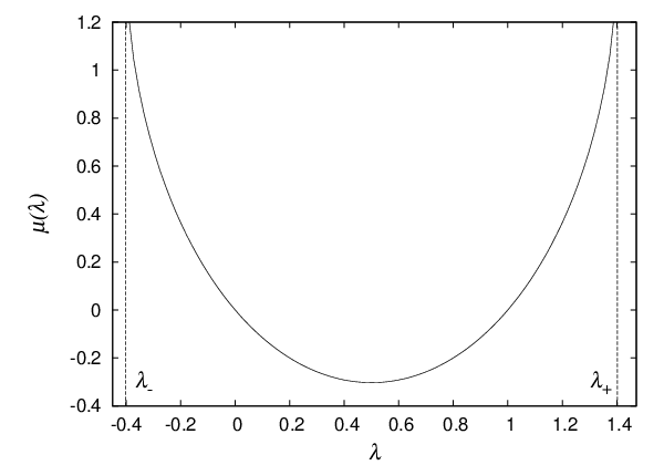
where the branch points are given by

\displaystyle\lambda_{\pm}=\frac{1}{2}\left[\frac{1}{T_{1}}-\frac{1}{T_{2}}\pm\sqrt{\left(\frac{1}{T_{1}}-\frac{1}{T_{2}}\right)^{2}+\frac{(\Gamma_{1}+\Gamma_{2})^{2}}{\Gamma_{1}\Gamma_{2}T_{1}T_{2}}}~\right];

(70)

note that $\lambda_{+}>0$ and $\lambda_{-}<0$ . In Fig. 2 we have depicted the large deviation function $\mu(\lambda)$ as a function of $\lambda$ .

The large deviation function $F(q)$ , $q=Q/t$ , characterizing the heat distribution, is determined parametrically from the large deviation function $\mu(\lambda)$ according to the Legendre transformation

	$\displaystyle q=\mu^{\prime}(\lambda)~\rightarrow~\lambda^{\ast}=\lambda(q),$		(71)
	$\displaystyle F(q)=\mu(\lambda^{\ast})-\lambda^{\ast}\mu^{\prime}(\lambda^{\ast}).$		(72)

We have, see also Visco [35],

\displaystyle F(q)=\frac{1}{2}\left[\Gamma_{1}+\Gamma_{2}-q(\lambda_{+}+\lambda_{-})-(\lambda_{+}-\lambda_{-})\sqrt{\Gamma_{1}\Gamma_{2}T_{1}T_{2}+q^{2}}~\right],~~

(73)

or inserting the branch points

\displaystyle F(q)=\frac{1}{2}\left[\Gamma_{1}+\Gamma_{2}-q\left(\frac{1}{T_{1}}-\frac{1}{T_{2}}\right)-\sqrt{\left(\frac{1}{T_{1}}-\frac{1}{T_{2}}\right)^{2}+\frac{(\Gamma_{1}+\Gamma_{2})^{2}}{\Gamma_{1}\Gamma_{2}T_{1}T_{2}}}\sqrt{\Gamma_{1}\Gamma_{2}T_{1}T_{2}+q^{2}}~\right].~~

(74)

Inspection of this equation shows that for small $q$ we have a displaced Gaussian distribution; for large $q$ we obtain exponential tails originating from the branch points $\lambda_{\pm}$ in $\mu(\lambda)$ , i.e.,

	$\displaystyle F(q)\sim-\lambda_{+}q~~\text{for}~~q\gg 0,$		(75)
	$\displaystyle F(q)\sim-\|\lambda_{-}\|\|q\|~~\text{for}~~q\ll 0.$		(76)

In Fig. 3 we have depicted the distribution function $P(Q/t)\propto\exp(tF(Q/t))$ , with $F(Q/t)$ given by (74), as a function of $Q/t$ on linear scales and log-linear scales (the inserts), for $\Gamma_{1}=1$ , $\Gamma_{2}=2$ , $T_{1}=1$ , $T_{2}=2$ , two different times $t_{\text{max}}=10,\,100$ , and two different values of the force constant $\kappa=1,\,10$ . We find good agreement between the simulations and the analytical results for the “central” part of the distribution. As expected, such an agreement improves as $t_{\text{max}}$ increases, being excellent for $t_{\text{max}}=100$ . The tails cannot be sampled by the simulations, as they correspond to rare trajectories, that would require a very large simulation time to be observed.

To further support our main finding, namely that the heat PDF is independent of the spring constant $\kappa$ , we calculated the first four moments of the distribution, over six orders on magnitudes of $\kappa$ , $10^{-2}\leq\kappa\leq 10^{4}$ . The simulations were run for $t_{\text{max}}=100$ , and $10^{5}$ independent trajectories were sampled. The results are reported in Fig. 4. In the left panel we plot the relative change $\left\langle Q^{m}(\kappa)\right\rangle/\left\langle Q^{m}(\kappa=0.01)\right\rangle$ , with $m=1\dots 4$ , and we find that the moments are practically constant over such a large range of values of $\kappa$ . Furthermore, for each value of $\kappa$ , we calculate the deviation $\epsilon_{m}$ of such moments from the expected value which reads:

\epsilon_{m}=\left|\frac{\left\langle Q_{\mathrm{num}}^{m}\right\rangle-\left\langle Q_{\mathrm{ex}}^{m}\right\rangle}{\left\langle Q^{m}_{\mathrm{ex}}\right\rangle}\right|,

(77)

where $\left\langle Q_{\mathrm{num}}^{m}\right\rangle$ is the $m$ -th moment as obtained by the numerical simulations, and $\left\langle Q_{\mathrm{ex}}^{m}\right\rangle$ is the corresponding exact value as obtained by equation (69). The quantities $\epsilon_{m}$ are plotted in the right panel of fig. 4. We find, that such deviations are negligible, basically due to numerical imprecision.

IV.1 Numerical investigation of the fourth-order potential case

In the present subsection, we investigate the heat PDF of a particle coupled to the two heath baths at temperature $T_{1}$ and $T_{2}$ , but moving in a quadratic potential

V_{4}(u)=a_{2}u^{2}+a_{4}u^{4}.

(78)

Thus in (9) the linear force is replaced by a term $2a_{2}u+4a_{4}u^{3}$ . We sample the heat PDF by considering $10^{5}$ independent trajectories, with $t_{\text{max}}=100$ , and choose different values for the parameters $a_{2}$ and $a_{4}$ in the potential (78). The results for the first four moments are reported in table 1, and they provide a strong evidence that also in this case the heat PDF, and so the large deviation function, is independent of the details of the underlying potential. As a bonus we also find that the first four moments are well described by the same large deviation function that we derived for the quadratic potential, which is independent of the potential details indeed, in the present case of the parameter $a_{2}$ and $a_{4}$ appearing in (78).

Table 1: Deviation

\epsilon_{m}

of the first four moments ((77)) from the values predicted by the substrate-independent large deviation function, (69). The quantities

a_{2}

and

a_{4}

are the parameters of the fourth-order potential

V_{4}

as given by (78).

$a_{2}$	$a_{4}$	$\epsilon_{1}$	$\epsilon_{2}$	$\epsilon_{3}$	$\epsilon_{4}$
$-3$	$1/2$	$1.1\times 10^{-3}$	$1.9\times 10^{-3}$	$2.5\times 10^{-3}$	$3.0\times 10^{-3}$
$-3/2$	$1/12$	$1.1\times 10^{-3}$	$1.6\times 10^{-3}$	$1.7\times 10^{-3}$	$1.6\times 10^{-3}$
$1$	$1$	$1.0\times 10^{-3}$	$1.3\times 10^{-3}$	$1.3\times 10^{-3}$	$1.0\times 10^{-3}$

V Discussion and conclusion

In this paper we have discussed a bound Brownian particle coupled to two distinct reservoirs, generalizing a model proposed by Derrida and Brunet [31]. The issue was to determine whether the presence of a harmonic trap has an effect on the heat transport between the reservoirs and on the large deviation function characterizing the long time heat distribution function. By a variety of analytical arguments based on a Langevin equation evaluation of the two lowest cumulants and an evaluation of the large deviation function by a direct method due to Derrida and Brunet, supported by a numerical simulation, we have demonstrated that the presence of a harmonic trap has no effect on the heat distribution function which has the same form as in the unbound case. This result is maybe intuitively evident since a single particle, in contrast to an extensive system, does not have internal degrees of freedom. Furthermore, we provide numerical evidence, that the heat distribution function is unchanged if we consider a fourth-order potential, again supporting our finding that such a distribution is independent of the underlying potential.

It also follows that the Gallavotti-Cohen fluctuation theorem [19] in (2) is unchanged by the presence of the spring. The fluctuation theorem is associated with the entropy production $Q_{1}/T_{1}$ and $Q_{2}/T_{2}$ at the heat sources whereas the presence of the spring represents a deterministic constraint not associated with entropy production [11, 31, 20].

Acknowledgements.

We are grateful to C. Mejia-Monasterio for many interesting discussions and for a critical reading of our manuscript. We also thank A. Mossa, A. Svane, and U. Poulsen for useful discussions. We thank B. Derrida and P. Visco for pointing out to us ref. [35]. We thank the Danish Centre for Scientific Computing for providing us with computational resources. The work of H. Fogedby has been supported by the Danish Natural Science Research Council under grant no. 436246.

References

[1] E. Trepagnier, C. Jarzynski, F. Ritort, G. Crooks, C. Bustamante, and J. Liphardt, Proc. Natl. Acad. Sci. USA 101, 15038 (2004)
[2] D. Collin, F. Ritort, C. Jarzynski, S. B. Smith, I. T. Jr, and C. Bustamante, Nature 437, 231 (2005)
[3] C. Tietz, S. Schuler, T. Speck, U. Seifert, and J. Wrachtrup, Phys. Rev. Lett. 97, 050602 (2006)
[4] V. Blickle, T. Speck, L. Helden, U.Seifert, and C. Bechinger, Phys. Rev. Lett. 96, 070603 (2006)
[5] G. Wang, E. Sevick, E. Mittag, D. J. Searles, and D. J. Evans, Phys. Rev. Lett. 89, 050601 (2002)
[6] A. Imparato, L. Peliti, G. Pesce, G. Rusciano, and A. Sasso, Phys. Rev. E 76, 050101R (2007)
[7] F. Douarche, S. Joubaud, N. B. Garnier, A. Petrosyan, and S. Ciliberto, Phys. Rev. Lett. 97, 140603 (2006)
[8] N. Garnier and S. Ciliberto, Phys. Rev. E 71, 060101(R) (2007)
[9] A. Imparato, P. Jop, A. Petrosyan, and S. Ciliberto, J. Stat. Mech, P10017(2008)
[10] C. Jarzynski, Phys. Rev. Lett. 78, 2690 (1997)
[11] J. Kurchan, J. Phys. A 31, 3719 (1998)
[12] G. Gallavotti, Phys. Rev. Lett. 77, 4334 (1996)
[13] G. E. Crooks, Phys. Rev. E 60, 2721 (1999)
[14] G. E. Crooks, Phys. Rev. E 61, 2361 (2000)
[15] U. Seifert, Phys. Rev. Lett. 95, 040602 (2005)
[16] U. Seifert, Europhys. Lett 70, 36 (2005)
[17] D. J. Evans, E. G. D. Cohen, and G. P. Morriss, Phys. Rev. Lett. 71, 2401 (1993)
[18] D. J. Evans and D. J. Searles, Phys. Rev. E 50, 1645 (1994)
[19] G. Gallavotti and E. G. D. Cohen, Phys. Rev. Lett. 74, 2694 (1995)
[20] J. L. Lebowitz and H. Spohn, J. Stat. Phys. 95, 333 (1999)
[21] P. Gaspard, J. Stat. Phys. 117, 599 (2004)
[22] A. Imparato and L. Peliti, Phys. Rev. E 74, 026106 (2006)
[23] R. van Zon and E. G. D. Cohen, Phys. Rev. Lett. 91, 110601 (2003)
[24] R. van Zon, S. Ciliberto, and E. G. D. Cohen, Phys. Rev. Lett. 92, 130601 (2004)
[25] R. van Zon and E. G. D. Cohen, Phys. Rev. 67, 046102 (2003)
[26] R. van Zon and E. G. D. Cohen, Phys. Rev. E 69, 056121 (2004)
[27] T. Speck and U. Seifert, Eur. Phys. J. B 43, 521 (2005)
[28] L. Rondoni and C. Mejía-Monasterio, Nonlinearity 20, R1 (2007)
[29] R. Chetrite and K. Gawe¿dzki, Communications in Mathematical Physics 282, 469 (2008)
[30] L. E. Reichl, A Modern Course in Statistical Physics (Wiley, New York, 1998)
[31] B. Derrida and E. Brunet, Einstein aujourd’hui (EDP Sciences, Les Ulis, 2005)
[32] C. V. den Broeck, R. Kawai, and P. Meurs, Phys. Rev. Lett. 93, 09060 (2004)
[33] M. van den Broeck and C. V. den Broeck, Phys. Rev. E 78, 011102 (2008)
[34] S. Lepri, R. Livi, and A. Politi, Phys. Rep. 377, 1 (2003)
[35] P. Visco, J. Stat. Mech., P06006(2006)
[36] J. Farago, J. Stat. Phys. 107, 781 (2002)
[37] J. Zinn-Justin, Quantum Field Theory and Critical Phenomena (Oxford University Press, Oxford, 1989)
[38] C. W. Gardiner, Handbook of Stochastic Methods (Springer-Verlag, New York, 1997)