Pulsed Adiabatic Photoassociation via Scattering Resonances
Abstract
We develop the theory for the Adiabatic Raman Photoassociation (ARPA) of ultracold atoms to form ultracold molecules in the presence of scattering resonances. Based on a computational method in which we replace the continuum with a discrete set of “effective modes”, we show that the existence of resonances greatly aids in the formation of deeply bound molecular states. We illustrate our general theory by computationally studying the formation of 85Rb2 molecules from pairs of colliding ultracold 85Rb atoms. The single-event transfer yield is shown to have a near-unity value for wide resonances, while the ensemble-averaged transfer yield is shown to be higher for narrow resonances. The ARPA yields are compared with that of (the experimentally measured) “Feshbach molecule” magneto-association. Our findings suggest that an experimental investigation of ARPA at sub-K temperatures is warranted.
I Introduction
Adiabatic Raman Photoassociation (ARPA) of ultracold atoms was introduced [1, 2, 3] as a practical way of producing ultracold diatomic molecules in their ground electronic and vib-rotational states. As illustrated in Fig.1, the method consists of photoassociating two colliding atoms by two (“dump” and “pump”) laser pulses that are mutually coherent and partially overlapping in space and time. As in three-level “Stimulated Raman Adiabatic Passage” (STIRAP) [4, 5, 6, 7, 8], one uses the “counter-intuitive” pulse ordering [4] in which the “dump” pulse, connecting the final bound state to an intermediate excited bound state, precedes the “pump” pulse, connecting the continuum to the latter state. In this way one executes a smooth “Adiabatic Passage” from an (ultracold atom-scattering) continuum to deeply bound molecular states [1, 2, 3].
The main problem with the above approach is the small “Franck-Condon” overlap factors between the intermediate bound state and the continuum. The introduction of a (“Feshbach”) resonance which is expected to better overlap with the intermediate bound state can alleviate this problem [9, 10]. As we show below, a Feshbach resonance also induces an important dynamic effect of prolonging the lifetime of the spatial region (the “Franck-Condon window”) in which photoassociation occurs. In this way a larger fraction of the atom pairs becomes available for photoassociation. This aspect has not been considered in previous works on photoassociation via Feshbach resonances [10], where it was concluded that wide resonances are more effective in promoting photoassociation than narrow ones. While we agree with Ref. [10] concerning the outcome of a single pair collision, we differ in our conclusions regarding the ensemble averaged yields: Based on our calculation of the number of recombining atoms per laser pulse-pair, we find that narrow resonances are in fact more effective than wide ones, because by prolonging the lifetime of the Franck Condon window, narrow resonances allow for more recombination events to occur. This mechanism more than compensates for the smaller energetic widths of the narrow resonances.
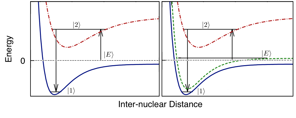
The structure of this paper is as follows: in section II we develop the working equations for the ARPA process, based on representing the continuum as a discrete set of “effective modes” [11]. In section III we present calculations of the ARPA population dynamics for a single pair of ultracold 85Rb atoms, and demonstrate how the FC window lifetime and spatial extent are being extended by the resonance. In section IV we compare the yield of ARPA with that of magneto-association [12, 13, 14, 15, 16] in which a pair of atoms in a Feshbach resonance are transformed into a stable molecule by sweeping over an external magnetic field, thereby pushing the resonance energy to lie below the molecular dissociation limit. We show that the two schemes lead to similar scaling of molecular production yield, but that ARPA is expected to be more efficient. Finally in the Appendix we show that the action of the pulses is tantamount to a quantum projective measurements on the initial continuum wave packet [2, 3]. Concluding remarks are provided in section V.
II Theory
II.1 The basic formulation
As illustrated in Fig.1, ARPA involves a -type level structure, similar to 3-state STIRAP, in which two, mutually coherent, temporally and spatially overlapping, laser pulses induce adiabatic passage from a molecular continuum (representing two colliding atoms) to the target bound level using an excited bound state as an intermediate. The Hamiltonian of the system is written as (in atomic units),
| (1) | |||||
| (2) |
is the “material” Hamiltonian. The bandwidth of the pulses ranges from being of order of 100K, down to tens of nK, which, when compared to the vibrational energy separation, makes it valid to include no other bound states than and . The second term in Eq.(1) describes the interaction of the transition dipole moment, with the “dump” () and “pump” () laser pulses, whose respective amplitudes and central frequencies are and . We tune , the pump center frequency, to be in near resonance with the transition frequency between the intermediate state and the continuum states ; and the dump center frequency, to be in resonance with the intermediate-to-final-state transition frequency. We assume that the laser fields do not vary significantly over the range of atom-atom distances in which photoassociation occurs, thereby justifying the elimination of the spatial variation of the fields.
As state we choose a deeply bound rovibrational level belonging to the ground electronic potential. Given this choice, the intermediate state taken to belong to an excited electronic potential, is chosen to be a vibrational state that overlaps well with the state. The main feature of the continuum we explore here is the embedding of a (Feshbach-type) resonance, leading to a sharp energy dependence of continuum-bound transition-dipole matrix elements [17, 9, 10].
Expanding the time-dependent system wave function in the material basis set,
| (3) |
we obtain, using the time-dependent Schrödinger’s equation the orthonormality of the material states and the Rotating Wave Approximation (RWA), that,
| (4) | |||||
| (5) | |||||
| (6) |
where is the continuum threshold energy, and are the detunings of the pulses, and is the spontaneous decay rate of state There are two Rabi frequencies in the problem, , and
Eq. (6) for representing a continuous set of equations for the continuously varying are numerically difficult to solve. We therefore eliminate Eq. (6) by integrating in time,
| (7) |
and substitute this formal solution into Eq. (5) to obtain that,
| (8) | |||||
By defining the source function, and the spectral auto-correlation function as
| (9) |
| (10) |
we can transform the above (continuous) set of differential equations to a set of two integro-differential equations,
| (11) |
The threshold energy in the source function will later in our analysis be taken as , since the function is zero near the collision threshold of the ground electronic potential, reflecting the density of states at zero kinetic energy.
II.2 The effective modes expansion
The simplest solution of Eqs. (11) is obtained by the “flat continuum” or “slowly varying continuum approximation” (SVCA), according to which, whenever varies sufficiently slowly with energy we replace it by its value at some average energy In this way the spectral auto-correlation function of Eq. (10) is reduced to and the integration in Eq. (11) is eliminated. Given this approximation, the dynamical equations assume, in matrix notation, the form,
| (12) |
where , , with T designating the transpose operation. The Hamiltonian matrix is defined as,
| (13) |
A detailed discussion of the solutions under SVCA was made in Refs. [1, 2, 3].
The SVCA is however invalid when collisional resonances are embedded in the continuum, because in that case changes rapidly near the resonance energy [17, 9]. In order to treat this case we parametrize as [11]
| (14) |
where represents the electronic transition dipole moment; - the Full-Width-at-Half-Maximum (FWHM); and - the centre-position of each resonance. This form is capable of approximating well both wide and narrow resonances [17, 10, 18]. As will be seen below, the above parametrization allows us to greatly simplify both the analytical theory as well as the numerical propagation of the dynamical equations.
With the expansion (14), the auto-correlation function in Eq. (10) can be evaluated analytically as,
| (15) |
with
| (16) |
Using Eq. (15) we now define [11] the “effective modes” variables as,
| (17) |
using which, we transform Eqs. (9) and (10) into,
| (18) | |||||
| (19) | |||||
| (20) |
In this way the original set of continuous equations for is replaced by a discrete set of equations for . We can further simplify the structure of the equations by defining , and mode-dependent Rabi frequencies, . With these definitions Eqs. (20) assume the form,
| (21) | |||||
| (22) | |||||
| (23) |
Writing these equations in matrix notation, we have that,
| (24) |
where
| (25) |
The “effective modes” amplitudes thus appear equivalent to some extra bound states of energies that are coupled by the Rabi frequencies to state , with detuning and decay rates as contained in . The non-Hermiticity of the Hamiltonian is due not just to the decay of the effective modes, appearing as the imaginary part of , but also to the Rabi frequencies , which are in general complex numbers, since the definition of involves a summation over , namely the effective interaction between overlapping resonances.

Eq. (24) resemble (multi-state) STIRAP [19] with and coupling respectively with , and with each of the effective modes (Fig. 2). We note however that the transfer dynamics differs in a significant way from ordinary STIRAP in that here the initial population does not reside in the effective modes, which get gradually populated. We can see this most explicitly for a single resonance, for which the dynamical equations assume the form,
| (26) | |||||
| (27) | |||||
| (28) |
By re-defining we obtain
| (29) | |||||
| (30) | |||||
| (31) |
where We see that here it is the terms in the square bracket that populates the effective mode (see Fig. 2).
Another contrast with three state STIRAP is the possibility of leakage of population from the “dark” state. In three states counter-intuitive pulse ordering adiabatic passage [4], the population resides initially in the adiabatic “dark” state, which is a superposition of the initial and target states only. In that case, the adiabaticity of the pulses guarantees the completeness of the transfer from the initial to the target state, leaving the intermediate state unpopulated at all times. Because in our case the effective mode gets populated in a gradual fashion, the system wave function may contain non-negligible contributions from other (“bright”) adiabatic states. These “bright” states have a small overlap with the intermediate state causing population to be lost via spontaneous emission.
III Computations of resonant photoassociation
We view the entire ARPA process as a statistical average over collisions between individual pairs of colliding atoms. As explained above, we represent such pairs by a set of (spatially extended) coherent wave packets arriving at the Franck Condon region at different times. The choice of coherent wave packets (rather than plane waves) as the basis of our our computations is merely a result of our wish to work with normalizeable states.
In this section we examine the above formulation by performing a set of computations on the resonantly enhanced photoassociation of ultracold 85Rb atoms to form 85Rb2 in its ground vibrational state. In keeping with our view of the process we divide the computations into two parts: (A) population transfer for each colliding pair, and (B) population transfer of the thermal ensemble of pairs of colliding atoms.
III.1 The single collision transfer yields

Following the model of Refs. [2, 3], we consider a pair of 85Rb atoms colliding on the ground electronic potential. We assume that at , chosen to occur before the onset of the pulses, all the population resides in the continuum wave packet and none in states or . The shape of the initial continuum wave packet of Eq. (3), with being the lower energetic limit (which is extended to ), is determined by the function, chosen here to be an energetically-narrow Gaussian [1, 2, 3]
| (32) |
with K and K. With this choice of parameters, the wave packet temporal peak occurs at s [1, 2]. The pair of pulses spectral widths are then chosen to have a good overlap with the energetic spread of the atomic wave packet. This requirement translates in the time domain to s pulse durations.
The scattering continuum is assumed to contain a narrow resonance, whose shape is given by Eq. (14). Figure 3 shows the shape of a resonance centred at K for 3 different widths. Since the (Feshbach) resonance position, can be tuned (magnetically), we can optimize the transfer by tuning to be always equal to . In this way one achieves the maximal FC enhancement (as confirmed by the numerical calculation presented in Figure 5 bottom panel).
The bound-to-bound matrix element is chosen to have a numeric value a.u. This numeric value can be different depending on the actual experimental set-up, but our results only depend on the Rabi frequency , which is proportional to the product of this bound-to-bound matrix element with the dump pulse amplitude. A increase (decrease) of the matrix element translates into a proportional decrease (increase) in the laser amplitude required. The spontaneous decay rate from level is ns [1, 2, 3]. The central frequency of the dump pulse is chosen to coincide with and the central frequency of the pump pulse - to coincide with . The field amplitudes and are taken as Gaussian functions, peaking, respectively, at s and s. The duration of both fields is s, and their peak intensity is W/cm2 [2].
With these specifications, Eqs. (21-23) simplify to yield,
| (33) | |||||
| (34) | |||||
| (35) |
where the Rabi frequencies are and . Notice here that the FC factors contained in and always appear as product with the field amplitudes . So the intensities of the dump and pump fields really are determined by the respective FC factors between the intermediate and target states, and between the continuum and the intermediate state. An enhancement on either of the the FC factors will result in the same order decrease in the laser amplitude (square-root of the intensity) needed.

In Fig. 4 we display the results of numerically integrating the equations for , and given that . We plot the populations of states and for a wide (K) resonance and a narrow (K) resonance. The most striking feature of this plot is that the wide resonance gives rise to an essentially complete population transfer (), while the transfer probability via the narrow resonance is only . Since the target state is the ground state, no loss of population can occur after a single photoassociation event. Loss of population is however possible when subsequent collisions with the gas of atoms and/or the action of subsequent pulses are considered. As shown in the lower panel, due to the adiabatic nature of the process and the “counter-intuitive” pulse ordering, the population of the intermediate level remains very low, even while the pulses are on.


III.2 Ensemble transfer yield
In agreement with Ref. [10], we have shown in sub-section A that for each event the transfer yield via a wide resonances is greater than that of a narrow resonances (Fig. 5 top panel). The situation is however different for an ensemble of colliding atoms, where, as we show below, the transfer yield of the narrow resonances is greater. The reason is that for narrow resonances the number of colliding pairs which can react to the light is greater, essentially because for narrower resonances one can work with narrower pulse bandwidths, hence longer pulses. The increase in the number of effective collisions occurring during the increased pulse durations, more than compensates for the reduction in the individual event transfer yield.
An alternative way of viewing this effect is to examine the role of the discrete effective modes which replace the continuum in our theory. These modes are to all intents and purposes resonances [20]. The only difference between the modes and scattering resonances is that the effective modes do not originate from a real bound state embedded in a continuum. Thus, as clearly seen in Eq. (35), the rate of de-populating an effective mode is proportional - the resonance-width of that mode. Hence narrower resonances, corresponding to smaller rates of depopulation, increase the interaction times of the effective modes with the intermediate level , thereby prolonging the duration of the Franck-Condon window.
In Fig. 6 we examine these trends in a quantitative way by displaying the field normalized source term, given as,
| (36) |
for resonances of changing widths. Clearly in evidence is the prolonged duration of when switching to narrower resonances.

The temporally stretched population source is also beneficial when we consider the action of a pulse pair that is delayed relative to the arrival time of the incoming wave packet. Figure 7 shows the transfer efficiency as a function of such delay times for 3 different resonance widths. For a narrow resonance, despite the drop in the peak value, the single collision transfer efficiency remains large for longer times. This means that atom pairs which started their collision at an earlier time can still be transformed into bound molecules with non-negligible probability.

delay time, where s is the pulses’ overlap peak time, and is the incoming wave packet peak time.

In order to obtain the delay times averaged molecular production yield for an atomic ensemble we need to calculate the area under the transfer-yield curves of Fig. 7. Figure 8 displays the dependence of the delay times averaged yield for various resonance widths. We first note that the yield changes relatively slowly for resonance width larger than K. This is because in this case the resonance width by far exceeds the energetic spread of the initial atomic ensemble and we approach the flat-continuum limit. As the width of the resonance drops to a few K, the molecular production yield rises to a maximum value, but drops significantly due to spontaneous emission for yet narrower resonances. Thus there exists an optimal resonance width for which the molecular production yield is maximal. Comparing the optimal molecular production yield, obtained for a (narrow) resonance value of K, with the yield in the flat-continuum limit, we see an improvement factor of 1.56.
III.3 Scaling behaviour with ensemble temperature
We now explore, as was done in Ref. [1], how the process varies as the average ensemble energy, and energy spread, are scaled down by a factor of , i.e., , and In ref. [1], we showed that the equations are invariant to this scaling provided the peak time was scaled up by the same factor and the initial wave packet amplitude is scaled as . We now consider the effect, in addition to the above, of scaling the resonance shape as . In order to match the spectral profile to the scaled , we need to scale up the centre frequencies and durations of the two pulses by the same factor. Since we can choose the intensity (amplitude) of the fields, we scale and [1] As a result, the source function scales like . The above scaling leaves the dynamical equations (Eqs. (33-35)), essentially unchanged, except for the spontaneous decay rate which cannot be scaled. As we scale the relevant times by a factor of , the deleterious effect of the spontaneous emission becomes more and more pronounced.


In Fig. 9 top panel we display the dependence of the single collision photoassociation yield on the spontaneous decay rate. Note that a change in one order of magnitude for the spontaneous decay rate only affects our results negligibly. When we compare the results to those displayed in Fig. 5 top panel, where the transfer yield is plotted as a function of the resonance width, we see that the transfer yield is not greatly affected at ensemble temperatures of a few K to a few K. As the ensemble temperature goes down by three orders of magnitude, the single collision transfer efficiency goes down too, by of its original value. The effect is more pronounced for narrower resonances, because the longer interaction times enhance the effect of the spontaneous decay. However, as shown in the lower panel of Fig. 9, it is possible to combat the effect of spontaneous decay at very low temperatures, e.g. in nK range, by increasing the amplitude (intensity) of both laser fields.
One can summarize these results by saying that the optimal resonance width is always of the ensemble temperature, and that the optimal molecular production efficiency by ARPA is higher than that of the wide resonance (flat continuum) case.
III.4 Thermalization
At long times the cumulative action of many pulses can change a region (or regions) in phase space corresponding to the recombining atoms, thereby affecting the initial wave packet amplitude However, an atomic ensemble can thermalize sufficiently fast, on the order of milliseconds, to yield the typical atomic trap setting of K temperature and /cm3 density [26]. This means (depending on the repetition rate of the pulses), that after a few thousand s pulse-pairs, the atomic ensemble can thermalize back to its original phase-space distribution, re-validating the ensemble-averaged form we used for .
According to previous estimates [1, 2], the total number of pulse pairs needed to transfer an entire atomic ensemble of density cm3 is around of . Therefore a few thousand pulses is indeed a very small fraction of total number of pulses needed, and the thermalization is fast comparing to the ensemble size molecular conversion time.
One is also inclined to pose the practical question of how to hide the newly formed molecule in state from subsequent pulse pairs. In accordance with more detailed discussions in Ref [1, 2], this can be done, for example, by allowing the newly formed molecules in state to “leak” away from the laser focus, which is possible because they react differently from the atoms to the confining laser frequency. A molecular trap can then be placed just below the atomic trap.
IV The ARPA yield dependence on the phase-space density and comparison to magneto-association.
Following Refs. [1, 3], we now present a detailed calculation of ARPA efficiency in a thermal ensemble. In order to estimate the fraction of atoms photoassociated per pulse-pair, we multiply , the single collision photoassociation probability at energy , by the number of collisions experienced by a given atom while the pulses are on. This is equivalent to averaging over all possible values of as performed above.
The number of collisions during the pulses is calculated as follows: at a given energy , the velocity of a given atom is and the distance traversed by it during a pulse of duration is . The cross-section for collision is where is the impact parameter. For -wave collisions, the semiclassical estimate is . Hence, the number of collisions experienced by the atom during the two pulses is where is the number of atoms in the trap, and is its volume. Putting all this together we obtain that the fraction of atoms photoassociated per pulse-pair is
| (37) |
Estimating the photoassociation yield for the case of flat continuum, we can set [3], and assume that all collisions occur at the temperature of the relative motion [24]. Further, when optimizing the yield for an atomic ensemble, we must choose because the bandwidths of the pump and dump pulses should match the energy spread in the ensemble. Thus we obtain
| (38) |
As pointed out above, a narrow resonance can enhance this fraction by a factor of , i.e., for a narrow resonance with given by Eq. (38).
We now consider the yield of magneto-association. In this process a time-varying external magnetic field is “swept” in magnitude, thereby moving the position of the Feshbach resonance of interest, to lie below the onset of the continuum. In this way the Feshbach resonance is stabilized to become a “Feshbach molecule” [12, 13, 14, 15, 16]. The magneto-association is then followed by a traditional 3-bound states STIRAP [15, 16].
The efficiency of this scheme is limited by the yield of the first step. In this step two atoms may form a molecule if prior to sweeping the magnetic field they are within, approximately, volume of phase space from each other [23]. Therefore at low to moderate phase space densities, the probability for a given atom to participate in a magneto-association process is
| (39) |
where is the single-particle phase space volume at temperature , and is the trap volume.
Comparing Eqs. (38) and (39) we see that the ARPA yield scales with temperature in exactly the same fashion as the magneto-association yield. However, in absolute numbers our estimates are that at low to moderate phase space densities the ARPA yield is times higher than the magneto-association yield. These findings strongly suggest that an experimental investigation of ARPA at sub-K temperatures is warranted.
V Conclusions
In this paper we have shown that Adiabatic Raman Photoassociation of ultracold atoms proceeding via collisional resonances is an efficient way of producing ultracold diatomic molecules in deeply bound states. We have done that by replacing the resonance-dominated molecular continuum by a discrete set of “effective modes” acting like a set of resonances. Though when the scattering resonance width is narrow it covers a smaller region in phase space (relative to the case of wide resonances), resulting in a drop of the single collision transfer efficiency, this drop is amply compensated for by the (as much as an order of magnitude) longer durations at which the photoassociating pulses can effectively act. In this way each pair of (pump and dump) laser pulses can act on more colliding atoms. The overall effect is that the narrow-resonances molecular production yield can be as much as higher than the wide resonances yield. For atomic temperatures in the K range, we find that the optimal conditions are attained for resonances whose widths are about 8 % of the ensemble temperature. We have also shown that the efficiency of the ARPA scheme compares favourably with the efficiency of magneto-association, with the yields of both schemes scaling with temperature in exactly the same manner. We have demonstrated that the ARPA process is a projective quantum measurement by the pulses of the initial continuum wave packet. This feature is a result of the single collision transfer efficiency being proportional to the degree of overlap between a function set by the pulses and the initial wave packet.
Future applications will deal with time-dependent resonances. We envision combining ARPA with a dynamical sweep of the Feshbach resonance across the threshold energy range. As the sweep will render the resonances narrower, the laser pulses will be made narrower so as to transfer the atomic gas into molecules in an optimal piecewise manner.
Appendix: ARPA as a projective measurement of the initial continuum wave function.
We showed in reference [2] that if the continuum is flat then ARPA implements a projective measurement of the initial wave function of two colliding atoms. Basically, the profiles of the laser pulses define a wave form that is adiabatically coupled to the target state . An initial scattering state which overlaps well will undergo population transfer to , while a state orthogonal to will not. By controlling the laser pulse profiles and implementing ARPA one is essentially measuring the wave function of the colliding atoms.
In this Appendix we extend the treatment to a resonance-dominated continuum, and relate the effect of collision resonances with our ability to control . We start by noting that in the adiabatic limit the solution of the equations of motion (12,13) is of the form [1, 2]
| (40) | |||||
| (41) | |||||
where
| (42) |
and
| (43) |
The final yield of the ARPA process is defined as the probability . Using Eqs. (42) and (43), we see that and the excited bound state amplitude indeed vanishes. Substituting and in Eq. (40) we obtain that
| (44) |
where
| (45) |
Thus the photoassociation amplitude is given as the projection of the source function onto the specific wave form whose shape is controlled by the amplitudes and the phases of and . Wave packets that are orthogonal to do not photoassociate in the ARPA process, while the ones that project well onto do. By tailoring the amplitudes and phases of the laser pulses, one can choose which continuum waveform is transferred into the target state [2].
In the main part of the paper we have shown that resonance dominated ARPA is most efficient when the resonance is narrow and the pump pulse has a narrow bandwidth relative to the initial ensemble temperature. These arguments allow us to replace in (9) by and obtain, via the convolution theorem,
| (46) |
where
| (47) |
and
| (48) |
is the phase-space envelope [21] of the initial wave packet of continuum states. Semiclassically it corresponds to the incoming wave function as a function of time measured at the turning point of a classical trajectory of energy . Positive values of - the time variable in the convolution integral of Eq. (46) - correspond to an outgoing motion, and negative values - to an incoming motion [21, 22].
The function the “FC window”, describes the residence time of the system in the “FC region,” the spatial region for which the FC factors are substantial. The temporal width at which is substantial, corresponds to the spatial extension of the FC window. In the flat continuum case, , and the time of residence in the FC region is zero. In contrast, a narrow resonance can cause the system to be greatly delayed in the FC window. In that case, an incoming continuum wave packet does not leave the Franck-Condon region right after entering it, but rather dwells there for the time given by the width .
We now consider the role of the continuum structure. Combining Eqs.(46) and (47) with (44), and introducing we obtain
| (49) |
where
| (50) |
Thus the shape of the wave form scooped from continuum by a laser pulse pair is equally defined by the laser pulses and by the continuum structure encoded in the window function .
Expanding the bound continuum transition spectrum into effective modes (Eq.(14)) we have
| (51) |
where is the Heaviside function. Therefore
| (52) |
Equations (44,52) present the main result of this section. They show that, similar to the case of a flat continuum, the profiles of the pump and dump pulses define the shape of coherent wave forms which can be transferred from the continuum into the target state. However the dwelling of the wave function due to the resonances decreases the ability to control these wave forms. If due to the resonances the dwell time exceeds the durations of the laser pulses, then by Eq.(50) we know that in addition to photoassociating atoms that arrive at the FC at there is a non-negligible probability to photoassociate atoms which get there before or after
VI Acknowledgements
Support by NSERC Discovery Grant, by a Major Thematic Grant from UBC’s Peter Wall Institute for Advanced Studies, and by the US DoD DTRA program are gratefully acknowledged. E.S. acknowledges the Institute of Theoretical Atomic, Molecular, and Optical Physics (ITAMP) for support during a visit to ITAMP facilities.
References
- [1] A. Vardi, D. Abrashkevich, E. Frishman, and M. Shapiro, J. Chem. Phys. 107, 6166 (1997).
- [2] E. A. Shapiro and M. Shapiro, “Adiabatic Raman Photoassociation with Shaped Laser Pulses”, Cold Molecules: Theory, Experiment, Applications, edited by R. Krems, W. Stwalley and B. Friedrich (Taylor and Francis, NY, 2009), p.291-316.
- [3] E. A. Shapiro, M. Shapiro, A. Pe’er, and J. Ye, Phys. Rev. A75, 013405 (2007).
- [4] N. V. Vitanov, M. Fleischhauer, B. W. Shore, and K. Bergmann,“Coherent Manipulation of Atoms and Molecules by Sequential Laser Pulses”, Adv. At., Mol., Opt.Phys. 46, 55 (2001).
- [5] J. Oreg, F. T. Hioe, and J. H. Eberly, Phys. Rev. A 29, 690-697 (1984).
- [6] U. Gaubatz, P. Rudecki, S. Sciemann, and K. Bergmann, J. Chem. Phys. 92, 5363-5376 (1990).
- [7] G. W. Coulston and K. Bergmann, J. Chem. Phys. 96, 3467-3475 (1992).
- [8] K. Bergmann, H. Theuer, and B. W. Shore, Rev. Mod. Phys. 70, 1003-1025 (1998).
- [9] P. Pellegrini, M. Gacesa, and R. Cote, Phys. Rev. Lett. 101, 053201 (2008).
- [10] E. Kuznetsova, M. Gacesa, P. Pellegrini, S. F. Yelin, R. Cote, New J. Phys. 11, 055028, 2009.
- [11] E. Frishman and M. Shapiro, Phys. Rev. A 54, 3310 (1996).
- [12] T. Kohler, K. Goral, and P. Julienne, Rev. Mod. Phys. 78, 1311 (2006).
- [13] E. Hodby, S. T. Thompson, C. A. Regal, M. Greiner, A. C. Wilson, D. S. Jin, E. A. Cornell, and C. E. Wieman , Phys. Rev. Lett. 94, 120402 (2005).
- [14] J. G. Danzl, E. Haller, M. Gustavsson, M. J. Mark, R. Hart, N. Bouloufa, O. Dulieu, H. Ritsch and Hanns-Christoph Nägerl, Science 321, 1062-1066 (2008).
- [15] K. -K. Ni, S. Ospelkaus, M. H. G. de Miranda, A. Pe’er, B. Neyenhuis, J. J. Zirbel, S. Kotochigova, P. S. Julienne, D. S. Jin and J. Ye, Science 322, 231-235 (2008).
- [16] J. G. Danzl, M. J. Mark, E. Haller, M. Gustavsson, R. Hart, J. Aldegunde, J. M. Hutson and Hanns-Christoph Nägerl, Nature Phys, 6, 265-270 (2010).
- [17] U. Fano, Phys. Rev. 124 1866 (1961).
- [18] X. Li, I. Thannopulos, and M. Shapiro, Phys. Rev. A, 83, 033415 (2011).
- [19] P. Král, I. Thanopulos, and M. Shapiro, Rev. Mod. Phys., 79, 53 (2007).
- [20] J. Taylor, “Scattering Theory” (John Wiley & Sons, Inc. New York, 1972).
- [21] E. A. Shapiro, Sov. Phys. JETP 118, 516 (2000); E. A. Shapiro, M. Spanner, and M. Yu. Ivanov, J. Mod. Optics 52, 897 (2005) and references therein; E. A. Shapiro, I. A Walmsley, and M. Yu. Ivanov , Phys. Rev. Lett. 98, 050501 (2007).
- [22] At ultracold temperatures the semiclassical point of view underlying the above carrier-envelope interpretation of the wave function is invalid for long range van-der-Waals interactions, i.e. at interatomic distances from several up to hundreds of atomic units. However, our approach predicts what happens to the wave function after the photoassociation is complete, at large interatomic distances where the semiclassical expression for the wave function is correct.
- [23] E. Hodby, S. T. Thompson, C. A. Regal, M. Greiner, A. C. Wilson, D. S. Jin, E. A. Cornell, and C. E. Wieman, Phys. Rev. Lett. 94, 120402 (2005).
- [24] The temperature of relative motion of identical atoms is twice the laboratory-frame temperature because the average squared velocity of the relative motion of two atoms is
- [25] A. Vardi, M. Shapiro, and J. R. Anglin, Phys. Rev. A 65, 027401 (2002).
- [26] K. W. Madison - private communication.