New Techniques for Upper-Bounding the ML Decoding Performance of Binary Linear Codes

Xiao Ma Jia Liu Baoming Bai ^†^†thanks: This work was presented in part at ISIT’2011.^†^†thanks: X.˜Ma and J. Liu are with the Department of Electronics and Communication Engineering, Sun Yat-sen University, Guangzhou 510275, China. (E-mail: maxiao@mail.sysu.edu.cn)^†^†thanks: B.˜Bai is with State Key Lab.˜of ISN, Xidian University, Xi’an 710071, China. (E-mail: bmbai@mail.xidian.edu.cn)

Abstract

In this paper, new techniques are presented to either simplify or improve most existing upper bounds on the maximum-likelihood (ML) decoding performance of the binary linear codes over additive white Gaussian noise (AWGN) channels. Firstly, the recently proposed union bound using truncated weight spectrum by Ma et al is re-derived in a detailed way based on Gallager’s first bounding technique (GFBT), where the “good region” is specified by a sub-optimal list decoding algorithm. The error probability caused by the bad region can be upper-bounded by the tail-probability of a binomial distribution, while the error probability caused by the good region can be upper-bounded by most existing techniques. Secondly, we propose two techniques to tighten the union bound on the error probability caused by the good region. The first technique is based on pair-wise error probabilities. The second technique is based on triplet-wise error probabilities, which can be upper-bounded by the fact that any three bipolar vectors form a non-obtuse triangle. The proposed bounds improve the conventional union bounds but have a similar complexity since they involve only the $Q$ -function. The proposed bounds can also be adapted to bit-error probabilities.

Index Terms:

Additive white Gaussian noise (AWGN) channel, binary linear block code, Gallager’s first bounding technique (GFBT), list decoding, maximum-likelihood (ML) decoding, union bound.

I Introduction

In most scenarios, there do not exist easy ways to compute the exact decoding error probabilities for specific codes and ensembles. Therefore, deriving tight analytical bounds is an important research subject in the field of coding theory and practice. Since the early 1990s, spurred by the successes of the near-capacity-achieving codes, renewed attentions have been paid to the performance analysis of the maximum-likelihood (ML) decoding algorithm. Though the ML decoding algorithm is prohibitively complex for most practical codes, tight bounds can be used to predict their performance without resorting to computer simulations. As shown in [1][2], most bounding techniques have connections to either the 1965 Gallager bound [3, 4, 5, 6] or the 1961 Gallager-Fano bound [7, 8, 9, 10, 11, 12, 13, 14, 15, 16, 17, 18]. This paper is relevant to the 1961 Gallager-Fano bound, which is also called Gallager’s first bounding technique (GFBT) in the literature. Our efforts focus on tightening the simplest conventional union bound, which is simple but loose and even diverges in the low-SNR region. Similar to many previously reported upper bounds surveyed in [2], our basic approach is based on GFBT

	$\displaystyle{\rm Pr}\{E\}$	$\displaystyle=$	$\displaystyle{\rm Pr}\{E,\underline{y}\in\mathcal{R}\}+{\rm Pr}\{E,\underline{y}\notin\mathcal{R}\}$		(1)
		$\displaystyle\leq$	$\displaystyle{\rm Pr}\{E,\underline{y}\in\mathcal{R}\}+{\rm Pr}\{\underline{y}\notin\mathcal{R}\},$		(2)

where $E$ denotes the error event, $\underline{y}$ denotes the received signal vector, and $\mathcal{R}$ denotes an arbitrary region around the transmitted signal vector which is usually interpreted as the “good region”. As pointed out in [2], the choice of the region $\mathcal{R}$ is very significant, and different choices of this region have resulted in various different improved upper bounds. Intuitively, the more similar the region $\mathcal{R}$ is to the Voronoi region of the transmitted codeword, the tighter the upper bound is. However, most existing improved upper bounds have higher computational complexity than the conventional union bound.

Different from most of the existing works, we define the good region using a list decoding algorithm. The basic idea is as follows. Upper bounds on the word-error probability for the list decoding algorithm (which is suboptimal) can also be applied to an ML decoding algorithm, while the list decoding algorithm can limit competitive candidate codewords.

Structure: The rest of this paper is organized as follows. In Sec. II, we present an upper bound of the angle formed by any three bipolar vectors, which will be used to upper-bound the triplet-wise error probabilities. In Sec. III, we re-derive, in a detailed way within the framework of the GFBT, the recently proposed union bound using truncated weight spectrum by Ma et al [19]. On one hand, the truncation technique is helpful when the whole weight spectrum is unknown or not computable. On the other hand, the truncation technique can be combined with any other upper-bounding techniques, potentially resulting in tighter upper bounds. In Sec. IV, we propose two techniques to improve the union bound. The first technique is based on the pair-wise error probabilities, which can be tightened by employing the independence of the error event and certain components of the received random vectors. The second technique is based on the triplet-wise error probabilities, which is shown to be a non-decreasing function of the angle formed by the transmitted codeword and the other two codewords. In Sec. V, the proposed bounds are adapted to ensembles of codes and bit-error probabilities. Numerical examples are provided in Sec. VI and we conclude this paper in Sec. VII.

II Preliminaries

II-A Geometrical Properties of Binary Codes

Let $\mathbb{F}_{2}=\{0,1\}$ and $\mathcal{A}_{2}=\{-1,+1\}$ be the binary field and the bipolar signal set, respectively. We use $W_{H}(\underline{v})$ to denote the Hamming weight of a binary vector $\underline{v}\stackrel{{\scriptstyle\Delta}}{{=}}(v_{0},v_{1},\cdots,v_{n-1})\in\mathbb{F}_{2}^{n}$ . We use $\|\underline{y}\|$ to denote the magnitude of a real vector $\underline{y}\stackrel{{\scriptstyle\Delta}}{{=}}(y_{0},y_{1},\cdots,y_{n-1})\in\mathbb{R}^{n}$ , that is, $\|\underline{y}\|=\sqrt{\sum_{0\leq t<n}y_{t}^{2}}$ . Let $\mathcal{C}[n,k]$ be a binary linear block code of dimension $k$ and length $n$ with a generator matrix $G$ of size ${k\times n}$ , that is,

\mathcal{C}\stackrel{{\scriptstyle\Delta}}{{=}}\left\{{\underline{c}}\in\mathbb{F}_{2}^{n}\mid{\underline{c}}={\underline{u}}G,{\underline{u}}\in\mathbb{F}_{2}^{k}\right\}.

(3)

Let $A_{i,j}$ denote the number of codewords $\underline{c}=\underline{u}G$ with $W_{H}(\underline{u})=i$ and $W_{H}(\underline{c})=j$ . Then $\{A_{j}\stackrel{{\scriptstyle\Delta}}{{=}}\sum_{i}A_{i,j}$ , $0\leq j\leq n\}$ is referred to as the weight spectrum of the given code $\mathcal{C}$ .

Consider the binary phase shift keying (BPSK) mapping $\phi:\mathbb{F}_{2}^{n}\mapsto\mathcal{A}_{2}^{n}$ taking $\underline{s}=\phi(\underline{v})$ by $s_{t}=1-2v_{t}$ for $0\leq t\leq n-1$ . The image of $\mathcal{C}$ under this mapping is denoted by $\mathcal{S}\stackrel{{\scriptstyle\Delta}}{{=}}\phi(\mathcal{C})$ . Hereafter, we may not distinguish $\underline{c}\in\mathcal{C}$ from its image $\underline{s}\in\mathcal{S}$ when representing a codeword. Let $d_{H}(\underline{v}^{(1)},\underline{v}^{(2)})\stackrel{{\scriptstyle\Delta}}{{=}}W_{H}(\underline{v}^{(1)}-\underline{v}^{(2)})$ be the Hamming distance between two binary vectors $\underline{v}^{(1)}$ and $\underline{v}^{(2)}$ . Then their Euclidean distance $\|\phi(\underline{v}^{(1)})-\phi(\underline{v}^{(2)})\|$ is equal to $2\sqrt{d_{H}(\underline{v}^{(1)},\underline{v}^{(2)})}$ . Obviously, the vectors in $\mathcal{A}_{2}^{n}$ (hence the bipolar codewords) are distributed on an $n$ -dimensional sphere of radius $\sqrt{n}$ centered at the origin $O$ of $\mathbb{R}^{n}$ . We have the following lemma.

Refer to caption — Fig. 1: Geometrical representation of three bipolar vectors.

Lemma 1

Let $\underline{u}$ , $\underline{v}$ and $\underline{w}$ be three bipolar vectors of length $n$ . Let $\theta$ be the angle formed by the two vectors $\overrightarrow{uv}\stackrel{{\scriptstyle\Delta}}{{=}}\underline{v}-\underline{u}$ and $\overrightarrow{uw}$ . Then we have

\theta\leq\min\left\{\frac{\pi}{2},~\arccos\sqrt{\frac{d_{1}}{n}}+\arccos\sqrt{\frac{d_{2}}{n}}\right\},

(4)

where $d_{1}=d_{H}(\underline{u},\underline{v})$ and $d_{2}=d_{H}(\underline{u},\underline{w})$ .

Proof:

To make the proof more readable, we have drawn the three bipolar vectors in a three-dimensional space, as shown in Fig. 1 (a). In essence, with a properly chosen orthogonal transformation, the three vectors can be viewed as three points in $\mathbb{R}^{3}$ (a three-dimensional subspace of $\mathbb{R}^{n}$ ). It should be noted that orthogonal transformations preserve inner products and (hence) lengths as well as angles.

It has been pointed out in [20] (without proof) that any three bipolar vectors form a non-obtuse triangle, which means $\theta\leq\pi/2$ . For completeness, we re-derive this bound in a detailed way. Let $\theta$ be the angle formed by $\overrightarrow{uv}$ and $\overrightarrow{uw}$ . It suffices to prove that the inner product $\overrightarrow{uv}\cdot\overrightarrow{uw}$ is non-negative. Actually, if $v_{t}\neq w_{t}$ , $(v_{t}-u_{t})(w_{t}-u_{t})=0$ since either $v_{t}=u_{t}$ or $w_{t}=u_{t}$ must hold; if $v_{t}=w_{t}$ , $(v_{t}-u_{t})(w_{t}-u_{t})\geq 0$ . Therefore

\overrightarrow{uv}\cdot\overrightarrow{uw}=\sum_{t}(v_{t}-u_{t})(w_{t}-u_{t})\geq 0.

(5)

To complete the proof of this lemma, consider the circumscribed circle of the triangle formed by the three points $\underline{u}$ , $\underline{v}$ and $\underline{w}$ (Fig. 1 (b)). Let $r$ be its radius. The angle can be written as $\theta=\theta_{1}+\theta_{2}$ , where $\cos\theta_{1}=\|\overrightarrow{uv}\|/(2r)$ and $\cos\theta_{2}=\|\overrightarrow{uw}\|/(2r)$ . It is then not difficult to verify that

\theta=\arccos\frac{\sqrt{d_{1}}}{r}+\arccos\frac{\sqrt{d_{2}}}{r}.

(6)

Noticing that the right hand side (RHS) of (6) is increasing with $r$ and that $r\leq\sqrt{n}$ , we have

\theta\leq\arccos\sqrt{\frac{d_{1}}{n}}+\arccos\sqrt{\frac{d_{2}}{n}}.

(7)

∎

II-B Union Bounds

Let $\underline{c}=(c_{0},c_{1},\cdots,c_{n-1})\in\mathcal{C}$ be a codeword. Suppose that $\underline{s}=\phi(\underline{c})$ is transmitted over an AWGN channel. Let $\underline{y}={\underline{s}}+{\underline{z}}$ be the received vector, where $\underline{z}$ is a vector of independent Gaussian random variables with zero mean and variance $\sigma^{2}$ . For AWGN channels, the ML decoding is equivalent to finding the nearest signal vector $\hat{\underline{s}}\in\mathcal{S}$ to $\underline{y}$ . A decoding error occurs whenever $\hat{\underline{s}}\neq\underline{s}$ . Let $E$ be the decoding error event (under ML decoding). Generally, it is a difficult task to calculate the decoding error probability ${\rm Pr}\{E\}$ . Hence one usually turns to bounding techniques. Due to the symmetry of the channel and the linearity of the code, the conditional error probability does not depend on the transmitted codeword, see, e.g., [21]. Therefore, without loss of generality, we assume that the all-zero codeword $\underline{c}^{(0)}$ is transmitted. The simplest upper bound is the union bound

$\displaystyle{\rm Pr}\left\{E\right\}$	$\displaystyle=$	$\displaystyle{\rm Pr}\left\{\bigcup_{d}E_{d}\right\}$	(8)
	$\displaystyle\leq$	$\displaystyle\sum_{d}{\rm Pr}\{E_{d}\}$
	$\displaystyle\leq$	$\displaystyle\sum_{d}A_{d}Q\left(\frac{\sqrt{d}}{\sigma}\right),$

where $E_{d}$ is the event that there exists at least one codeword of Hamming weight $d\geq 1$ that is nearer than $\underline{c}^{(0)}$ to $\underline{y}$ , and $Q\left(\frac{\sqrt{d}}{\sigma}\right)$ is the pair-wise error probability with

Q(x)\stackrel{{\scriptstyle\Delta}}{{=}}\int_{x}^{+\infty}\frac{1}{\sqrt{2\pi}}e^{-\frac{z^{2}}{2}}\,{\rm d}z.

(9)

The question is, how many terms do we need to count for the summation in the above bound? If too few terms are counted, we will obtain a lower bound of the upper bound, which may be neither an upper bound nor a lower bound; if too many are counted, we need pay more efforts to compute the distance distribution and only a loose upper bound will be obtained. To get a tight upper bound, we may determine the terms by analyzing the facets of the Voronoi region of the codeword $\underline{c}^{(0)}$ [22] [20], which is a difficult task for a general code.

It is well-known that the conventional union bound is loose and even diverges ( $\geq 1$ ) in the low-SNR region. One objective of this paper is, without too much complexity increase, to reduce the number of involved terms in the conventional union bound. The other objective of this paper is to tighten the bound on ${\rm Pr}\{E_{d}\}$ , which used to be upper-bounded by the pair-wise error probability, where intersections of half-spaces related to codewords other than the transmitted one are counted more than once. For some of well-known existing improved bounds based on GFBT, such as the sphere bound (SB), the tangential-sphere bound (TSB) and the Divsalar bound, see the monograph [2, Ch. 3] and the references therein.

III Upper Bounds Using Truncated Weight Spectrum

Recently, Ma et al [19] proposed a union bound which involves only truncated weight spectrum. In this section, we re-derive this “truncated” union bound within the framework of GFBT, where the region $\mathcal{R}$ is defined in an unusual way based on the following conceptual suboptimal list decoding algorithm.

Algorithm 1

(A list decoding algorithm for the purpose of performance analysis)

S1.

Make hard decisions, i.e., for $0\leq t\leq n-1$ ,

$\hat{y}_{t}=\left\{\begin{array}[]{cc}0,&y_{t}>0\\ 1,&y_{t}\leq 0\end{array}\right..$ (10)

Then the channel $c_{t}\rightarrow\hat{y}_{t}$ becomes a memoryless binary symmetric channel (BSC) with cross probability $p_{b}\stackrel{{\scriptstyle\Delta}}{{=}}Q\left(\frac{1}{\sigma}\right)$ .
S2.

List all codewords within the Hamming sphere with center at $\underline{\hat{y}}$ of radius $d^{*}\geq 0$ . The resulting list is denoted as $\mathcal{L}_{\underline{y}}$ .
S3.

If $\mathcal{L}_{\underline{y}}$ is empty, declare a decoding error; otherwise, find the codeword $\underline{c}^{*}\in\mathcal{L}_{\underline{y}}$ such that $\phi(\underline{c}^{*})\in\mathcal{S}$ is closest to $\underline{y}$ .

❑

Now we define

\mathcal{R}\stackrel{{\scriptstyle\Delta}}{{=}}\left\{\underline{y}|{\underline{c}}^{(0)}\in\mathcal{L}_{\underline{y}}\right\}.

(11)

In words, the region $\mathcal{R}$ consists of all those $\underline{y}$ having at most $d^{*}$ non-positive components. The decoding error occurs in two cases under the assumption that the all-zero codeword ${\underline{c}}^{(0)}$ is transmitted.

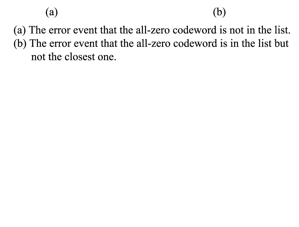
Case 1. The all-zero codeword is not in the list $\mathcal{L}_{\underline{y}}$ (see Fig. 2 (a)), that is, $\underline{y}\notin\mathcal{R}$ , which means that at least $d^{*}+1$ errors occur over the BSC. This probability is

{\rm Pr}\{\underline{y}\notin\mathcal{R}\}=\sum_{m=d^{*}+1}^{n}\binom{n}{m}p_{b}^{m}(1-p_{b})^{n-m}.

(12)

Case 2. The all-zero codeword is in the list $\mathcal{L}_{\underline{y}}$ , but is not the closest one to $\underline{y}$ (see Fig. 2 (b)), which is equivalent to the event $\left\{E,\underline{y}\in\mathcal{R}\right\}$ . This probability is upper-bounded by

{\rm Pr}\left\{E,\underline{y}\in\mathcal{R}\right\}\leq{\rm Pr}\left\{\bigcup_{d\leq 2d^{*}}E_{d},\;\;\underline{y}\in\mathcal{R}\right\}

(13)

since all codewords in the list $\mathcal{L}_{\underline{y}}$ are at most $2d^{*}$ away from the all-zero codeword and not all codewords of a specific weight are in the list. The above upper bound involves only truncated weight spectrum. However, the region $\mathcal{R}$ is in unknown shape and may not be symmetric, which causes difficulties when computing the upper bound. To circumvent this difficulty, we may enlarge $\mathcal{R}$ to $\mathbb{R}^{n}$ and get

$\displaystyle{\rm Pr}\left\{E,\underline{y}\in\mathcal{R}\right\}$	$\displaystyle\leq$	$\displaystyle{\rm Pr}\left\{\bigcup_{d\leq 2d^{*}}E_{d},\;\;\underline{y}\in\mathcal{R}\right\}$	(14)
	$\displaystyle\leq$	$\displaystyle{\rm Pr}\left\{\bigcup_{d\leq 2d^{*}}E_{d},\;\;\underline{y}\in\mathbb{R}^{n}\right\}$	(15)
	$\displaystyle=$	$\displaystyle{\rm Pr}\left\{\bigcup_{d\leq 2d^{}}E_{d}\right\}\leq T_{u}(\mathcal{C}_{2d^{}}),$	(16)

where $T_{u}(\mathcal{C}_{2d^{*}})$ is a computable upper bound on ${\rm Pr}\left\{\bigcup_{d\leq 2d^{*}}E_{d}\right\}$ , which depends only on the sub-code $\mathcal{C}_{2d^{*}}$ consisting of all codewords with Hamming weight no greater than $2d^{*}$ . It is worth pointing out that, although the sub-code $\mathcal{C}_{2d^{*}}$ may not be linear, most bounding techniques in [2] can be applied to $\mathcal{C}_{2d^{*}}$ to get such an upper bound under the assumption that the all-zero codeword is transmitted. Hereafter, we use the notation $\mathcal{C}_{t}\stackrel{{\scriptstyle\Delta}}{{=}}\left\{{\underline{c}}\in\mathcal{C}\mid W_{H}(\underline{c})\leq t\right\}$ .

For convenience, we define

B(p,N_{t},N_{\ell},N_{u})\stackrel{{\scriptstyle\Delta}}{{=}}\sum_{m=N_{\ell}}^{N_{u}}\binom{N_{t}}{m}p^{m}(1-p)^{N_{t}-m}.

(17)

The function $B(p,N_{t},N_{\ell},N_{u})$ , which will be used over and over again in this paper, is just the probability that the number of bit-errors occurring in a binary vector of total length $N_{t}$ , when passing through a BSC with cross error probability $p$ , ranges from $N_{\ell}$ to $N_{u}$ . Note that $B(p,N_{t},N_{\ell},N_{u})$ can be calculated recursively independently of codes.

Combining (12), (16) and (17) with (2), we get an upper bound

{\rm Pr}\left\{E\right\}\leq T_{u}(\mathcal{C}_{2d^{*}})+B(p_{b},n,d^{*}+1,n),

(18)

where the second term in the RHS is computable without requiring the code structure and the first term depends only on the sub-code $\mathcal{C}_{2d^{*}}$ .

On one hand, similar to the SB [10] and the TSB [11], the proposed upper bound (18) involves only truncated weight spectrum, which is hence helpful when the whole weight spectrum is not computable. On the other hand, if the complete weight spectrum is available, the proposed bounding technique can potentially improve any existing upper bounds.

Proposition 1

Let $T_{u}$ be an upper-bounding technique. We have

{\rm Pr}\left\{E\right\}\leq\min_{0\leq d^{*}\leq n}\left\{T_{u}(\mathcal{C}_{2d^{*}})+B(p_{b},n,d^{*}+1,n)\right\},

(19)

which delivers an upper bound strictly less than 1 and not looser than any existing upper bounds $T_{u}(\mathcal{C})$ .

Proof:

Noting that $T_{u}(\mathcal{C}_{0})=0$ and $B(p_{b},n,1,n)=1-(1-p_{b})^{n}$ , we have, by setting $d^{*}=0$ ,

\displaystyle{\rm Pr}\left\{E\right\}<1.

(20)

Similarly, noting that $T_{u}(\mathcal{C}_{2n})=T_{u}(\mathcal{C})$ and $B(p_{b},n,n+1,n)=0$ , we have, by setting $d^{*}=n$ ,

\displaystyle{\rm Pr}\left\{E\right\}\leq T_{u}(\mathcal{C}).

(21)

∎

Taking the conventional union bound as $T_{u}$ , we have

Theorem 1

Let $d_{\min}$ be the minimum Hamming weight of the code $\mathcal{C}$ . We have

{\rm Pr}\left\{E\right\}\leq\min_{0\leq d^{*}\leq n}\left\{\sum_{d_{\min}\leq d\leq 2d^{*}}A_{d}Q\left(\frac{\sqrt{d}}{\sigma}\right)+B(p_{b},n,d^{*}+1,n)\right\}.

(22)

Proof:

It can be proved by substituting the conventional union bound for $T_{u}(\mathcal{C}_{2d^{*}})$ (in the same form as shown in (8)) into (19). ∎

Remark. The bound (22), which is slightly different from that proposed in [19], requires higher computational loads than the conventional union bound. The overhead is caused by recursively computing $B(p_{b},n,d^{*}+1,n)$ and minimizing over $d^{*}$ . If we do not perform the optimization and simply set $d^{*}=n$ , we get the conventional union bound, implying that the technique can potentially improve the conventional union bound, as stated in Proposition 1.

IV Improved Union Bounds

We have interpreted the “truncated” union bound as an upper-bounding technique based on the GFBT, where the region $\mathcal{R}$ is defined by a sub-optimal decoding algorithm. To bound ${\rm Pr}\{E,{\underline{y}}\in\mathcal{R}\}$ , we have enlarged $\mathcal{R}$ to $\mathbb{R}^{n}$ , as shown in the derivation from (14) to (15). The objective of this section is to reduce the effect of such an enlargement.

Noticing that the event $\underline{y}\in\mathcal{R}$ is equivalent to the event $W_{H}(\underline{\hat{y}})\leq d^{*}$ , we have

Proposition 2

{\rm Pr}\{E\}\leq\min_{0\leq d^{*}\leq n}\left\{\sum\limits_{d\leq 2d^{*}}{\rm Pr}\left\{E_{d},W_{H}(\underline{\hat{y}})\leq d^{*}\right\}+B(p_{b},n,d^{*}+1,n)\right\}.

(23)

Proof:

For any $d^{*}$ ( $0\leq d^{*}\leq n$ ),

$\displaystyle{\rm Pr}\{E\}$	$\displaystyle\leq$	$\displaystyle{\rm Pr}\{E,\underline{y}\in\mathcal{R}\}+{\rm Pr}\{\underline{y}\notin\mathcal{R}\}$	(24)
	$\displaystyle\leq$	$\displaystyle{\rm Pr}\left\{\bigcup_{d\leq 2d^{}}E_{d},W_{H}(\underline{\hat{y}})\leq d^{}\right\}+B(p_{b},n,d^{*}+1,n)$
	$\displaystyle\leq$	$\displaystyle\sum\limits_{d\leq 2d^{}}{\rm Pr}\left\{E_{d},W_{H}(\underline{\hat{y}})\leq d^{}\right\}+B(p_{b},n,d^{*}+1,n).$

∎

In this section, we focus on how to upper-bound ${\rm Pr}\left\{E_{d},W_{H}(\underline{\hat{y}})\leq d^{*}\right\}$ for any given $d$ and $d^{*}$ . Without loss of generality, we assume that $A_{d}\geq 1$ and denote all the codewords with weight $d$ by $\underline{c}^{(\ell)}$ , $1\leq\ell\leq A_{d}$ . Let $E_{0\rightarrow\ell}$ be the event that $\underline{c}^{(\ell)}$ is nearer than ${\underline{c}}^{(0)}$ to $\underline{y}$ .

IV-A Union Bounds Using Pair-Wise Error Probability

Lemma 2

{\rm Pr}\left\{E_{0\rightarrow 1},W_{H}(\underline{\hat{y}})\leq d^{*}\right\}\leq Q(\sqrt{d}/\sigma)B\left(p_{b},n-d,0,d^{*}-1\right).

(25)

Proof:

Without loss of generality, let ${\underline{c}}^{(1)}\stackrel{{\scriptstyle\Delta}}{{=}}(\underbrace{1\cdots 1}_{d}\underbrace{0\cdots 0}_{n-d})$ . Denote $\underline{y}_{0}^{d-1}\stackrel{{\scriptstyle\Delta}}{{=}}(y_{0},\cdots,y_{d-1})$ and $\underline{y}_{d}^{n-1}\stackrel{{\scriptstyle\Delta}}{{=}}(y_{d},\cdots,y_{n-1})$ . Evidently, only $\underline{y}_{0}^{d-1}$ can cause the decoding error event that ${\underline{c}}^{(1)}$ is nearer than ${\underline{c}}^{(0)}$ to $\underline{y}$ . In other words, the event $E_{0\rightarrow 1}$ is independent of ${\underline{y}}_{d}^{n-1}$ and ${\rm Pr}\{E_{0\rightarrow 1}\}=Q\left(\sqrt{d}/\sigma\right)$ . Also notice that the received signal vector $\underline{y}$ which can cause the event $E_{0\rightarrow 1}$ must satisfy $W_{H}(\hat{\underline{y}}_{0}^{d-1})\geq 1$ . Hence $\left\{{\underline{y}}|E_{0\rightarrow 1},W_{H}(\underline{\hat{y}})\leq d^{*}\right\}\subseteq\left\{{\underline{y}}|E_{0\rightarrow 1},W_{H}(\hat{\underline{y}}_{d}^{n-1})\leq d^{*}-1\right\}$ . Then we have

$\displaystyle{\rm Pr}\left\{E_{0\rightarrow 1},W_{H}(\underline{\hat{y}})\leq d^{*}\right\}$	$\displaystyle\leq$	$\displaystyle{\rm Pr}\left\{E_{0\rightarrow 1},W_{H}(\hat{\underline{y}}_{d}^{n-1})\leq d^{*}-1\right\}$	(26)
	$\displaystyle=$	$\displaystyle{\rm Pr}\left\{E_{0\rightarrow 1}\right\}{\rm Pr}\left\{W_{H}(\hat{\underline{y}}_{d}^{n-1})\leq d^{*}-1\right\}$	(27)
	$\displaystyle=$	$\displaystyle Q(\sqrt{d}/\sigma)B\left(p_{b},n-d,0,d^{*}-1\right).$	(28)

∎

Theorem 2

{\rm Pr}\left\{E_{d},W_{H}(\underline{\hat{y}})\leq d^{*}\right\}\leq A_{d}Q(\sqrt{d}/\sigma)B\left(p_{b},n-d,0,d^{*}-1\right).

(29)

Proof:

By union bounds and the symmetries of the error events,

$\displaystyle{\rm Pr}\left\{E_{d},W_{H}(\underline{\hat{y}})\leq d^{*}\right\}$	$\displaystyle=$	$\displaystyle{\rm Pr}\left\{\bigcup_{1\leq\ell\leq A_{d}}E_{0\rightarrow\ell},W_{H}(\underline{\hat{y}})\leq d^{*}\right\}$	(30)
	$\displaystyle\leq$	$\displaystyle\sum\limits_{1\leq\ell\leq A_{d}}{\rm Pr}\left\{E_{0\rightarrow\ell},W_{H}(\underline{\hat{y}})\leq d^{*}\right\}$	(31)
	$\displaystyle=$	$\displaystyle A_{d}{\rm Pr}\left\{E_{0\rightarrow 1},W_{H}(\underline{\hat{y}})\leq d^{*}\right\}$	(32)
	$\displaystyle\leq$	$\displaystyle A_{d}Q(\sqrt{d}/\sigma)B\left(p_{b},n-d,0,d^{*}-1\right).$	(33)

∎

IV-B Union Bounds Using Triplet-Wise Error Probability

Temporarily, we assume that $A_{d}\geq 2$ is even. Then we have

\displaystyle{\rm Pr}\{E_{d},W_{H}(\hat{\underline{y}})\leq d^{*}\}

\displaystyle\leq

\displaystyle\sum_{1\leq\ell\leq A_{d}/2}{\rm Pr}\left\{E_{0\rightarrow(2\ell-1)}\bigcup E_{0\rightarrow 2\ell},W_{H}(\hat{\underline{y}})\leq d^{*}\right\}.

(34)

If we can find ways to calculate or upper-bound ${\rm Pr}\left\{E_{0\rightarrow(2\ell-1)}\bigcup E_{0\rightarrow 2\ell},W_{H}(\hat{\underline{y}})\leq d^{*}\right\}$ , we may improve the conventional union bound.

In this paper, we refer to the probability ${\rm Pr}\left\{E_{0\rightarrow 1}\bigcup E_{0\rightarrow 2}\right\}$ as triplet-wise error probability. We have the following lemma.

Lemma 3

Let $\underline{c}^{(0)}$ be the all-zero codeword with bipolar image $\underline{s}^{(0)}$ . Let $\underline{c}^{(1)}$ and $\underline{c}^{(2)}$ be the codewords of Hamming weight $d$ with bipolar images $\underline{s}^{(1)}$ and $\underline{s}^{(2)}$ , respectively. The triplet-wise error probability

{\rm Pr}\left\{E_{0\rightarrow 1}\bigcup E_{0\rightarrow 2}\right\}=Q(\sqrt{d}/\sigma)+\int_{\sqrt{d}}^{+\infty}f(\xi_{1})\int_{-\infty}^{\frac{\sqrt{d}-\xi_{1}\cos\theta}{\sin\theta}}f(\xi_{2})~{\rm d}\xi_{2}~{\rm d}\xi_{1},

(35)

where $f(x)=\frac{1}{\sqrt{2\pi}\sigma}e^{-x^{2}/(2\sigma^{2})}$ is the probability density function of $\mathcal{N}(0,\sigma^{2})$ and $\theta$ is the angle formed by the two vectors $\overrightarrow{\underline{s}^{(0)}\underline{s}^{(1)}}$ and $\overrightarrow{\underline{s}^{(0)}\underline{s}^{(2)}}$ . Furthermore, the triplet-wise error probability is a non-decreasing function of $\theta$ .

Proof:

Similar to the proof of Lemma 1, we have sketched the two vectors $\overrightarrow{\underline{s}^{(0)}\underline{s}^{(1)}}$ and $\overrightarrow{\underline{s}^{(0)}\underline{s}^{(2)}}$ in a two-dimensional space, as shown in Fig. 3, where we have chosen $\underline{s}^{(0)}$ as the origin $O$ and arranged $\overrightarrow{\underline{s}^{(0)}\underline{s}^{(1)}}$ on the abscissa axis $\overrightarrow{O\xi_{1}}$ .

Assume that ${\underline{s}}^{(0)}$ is transmitted and $\underline{y}={\underline{s}}^{(0)}+{\underline{z}}$ is received, where $\underline{z}$ is a sample from a random vector $\underline{Z}$ whose components are independent and identically distributed as $\mathcal{N}(0,\sigma^{2})$ . Let $Z_{\xi_{1}}$ and $Z_{\xi_{2}}$ be the two independent Gaussian random variables by projecting $\underline{Z}$ onto the abscissa axis and ordinate axis, respectively. Specifically, say, $Z_{\xi_{1}}$ is the inner product $\langle{\underline{Z}},\frac{\underline{s}^{(1)}-\underline{s}^{(0)}}{\|\underline{s}^{(1)}-\underline{s}^{(0)}\|}\rangle$ . It is well-known that only $(Z_{\xi_{1}},Z_{\xi_{2}})$ can cause the error event $\{E_{0\rightarrow 1}\bigcup E_{0\rightarrow 2}\}$ . Actually, as shown in Fig. 3, the error event $\{E_{0\rightarrow 1}\bigcup E_{0\rightarrow 2}\}$ occurs if and only if the vector $(Z_{\xi_{1}},Z_{\xi_{2}})$ falls into the shaded region, which can be partitioned into

	$\displaystyle\mathcal{R}_{1}$	$\displaystyle\stackrel{{\scriptstyle\Delta}}{{=}}$	$\displaystyle\left\{(\xi_{1},\xi_{2})\|\xi_{1}\geq\sqrt{d},~\xi_{1}\cos\theta+\xi_{2}\sin\theta<\sqrt{d}\right\},$		(36)
	$\displaystyle\mathcal{R}_{2}$	$\displaystyle\stackrel{{\scriptstyle\Delta}}{{=}}$	$\displaystyle\left\{(\xi_{1},\xi_{2})\|\xi_{1}\cos\theta+\xi_{2}\sin\theta\geq\sqrt{d}\right\}.$		(37)

Since ${\rm Pr}\{\mathcal{R}_{1}\}=\int_{\sqrt{d}}^{+\infty}f(\xi_{1})\int_{-\infty}^{\frac{\sqrt{d}-\xi_{1}\cos\theta}{\sin\theta}}f(\xi_{2})~{\rm d}\xi_{2}~{\rm d}\xi_{1}$ and ${\rm Pr}\{\mathcal{R}_{2}\}=Q(\sqrt{d}/\sigma)$ , we have

	$\displaystyle{\rm Pr}\left\{E_{0\rightarrow 1}\bigcup E_{0\rightarrow 2}\right\}$	$\displaystyle=$	$\displaystyle{\rm Pr}\{\mathcal{R}_{1}\}+{\rm Pr}\{\mathcal{R}_{2}\}$		(38)
		$\displaystyle=$	$\displaystyle\int_{\sqrt{d}}^{+\infty}f(\xi_{1})\int_{-\infty}^{\frac{\sqrt{d}-\xi_{1}\cos\theta}{\sin\theta}}f(\xi_{2})~{\rm d}\xi_{2}~{\rm d}\xi_{1}+Q(\sqrt{d}/\sigma).$		(38)

To prove the monotonicity, it suffices to prove that $\frac{\sqrt{d}-\xi_{1}\cos\theta}{\sin\theta}$ increases with $\theta$ for $\xi_{1}\geq\sqrt{d}$ . This can be verified by noting that its derivative $\frac{\xi_{1}-\sqrt{d}\cos\theta}{\sin^{2}\theta}\geq 0$ for $\xi_{1}\geq\sqrt{d}$ . ∎

Lemma 4

For any two codewords ${\underline{c}}^{(1)}$ and ${\underline{c}}^{(2)}$ of Hamming weight $d$ , the triplet-wise error probability¹¹ 1 As pointed out by an anonymous reviewer that the RHS of (39) is the same as the symbol error probability of quadrature phase shift keying (QPSK) over AWGN channels [23].

{\rm Pr}\left\{E_{0\rightarrow 1}\bigcup E_{0\rightarrow 2}\right\}\leq 2Q(\sqrt{d}/\sigma)-Q^{2}(\sqrt{d}/\sigma).

(39)

Proof:

From Lemmas 1 and 3, we can substitute $\theta=\pi/2$ into (35) to complete the proof. ∎

Remark. From Lemmas 1 and 3, in the case of $\arccos{\sqrt{\frac{d}{n}}}<\pi/4$ , we may substitute $\theta=2\arccos{\sqrt{\frac{d}{n}}}$ into (35) to get a tighter bound, however, which needs higher computational loads.

Lemma 5

For any two codewords ${\underline{c}}^{(1)}$ and ${\underline{c}}^{(2)}$ of Hamming weight $d$ ,

{\rm Pr}\left\{E_{0\rightarrow 1}\bigcup E_{0\rightarrow 2},W_{H}(\hat{\underline{y}})\leq d^{*}\right\}\leq\left(2Q(\sqrt{d}/\sigma)-Q^{2}(\sqrt{d}/\sigma)\right)B(p_{b},n-2d,0,d^{*}-1).

(40)

Proof:

Without loss of generality, assume that

{\underline{c}}^{(1)}\stackrel{{\scriptstyle\Delta}}{{=}}(c_{0}^{(1)}\cdots c_{2d-1}^{(1)}\underbrace{0\cdots 0}_{n-2d})

(41)

and

{\underline{c}}^{(2)}\stackrel{{\scriptstyle\Delta}}{{=}}(c_{0}^{(2)}\cdots c_{2d-1}^{(2)}\underbrace{0\cdots 0}_{n-2d}).

(42)

Then only ${\underline{y}}_{0}^{2d-1}$ can cause the event that ${\underline{c}}^{(1)}$ or ${\underline{c}}^{(2)}$ are nearer than ${\underline{c}}^{(0)}$ to $\underline{y}$ . Also notice that the received signal vector $\underline{y}$ which can cause the event $E_{0\rightarrow 1}\bigcup E_{0\rightarrow 2}$ must satisfy $W_{H}(\hat{\underline{y}}_{0}^{2d-1})\geq 1$ . Hence $\left\{{\underline{y}}|E_{0\rightarrow 1}\bigcup E_{0\rightarrow 2},W_{H}(\underline{\hat{y}})\leq d^{*}\right\}\subseteq\left\{{\underline{y}}|E_{0\rightarrow 1}\bigcup E_{0\rightarrow 2},W_{H}(\hat{\underline{y}}_{2d}^{n-1})\leq d^{*}-1\right\}$ . Then we have

$\displaystyle{\rm Pr}\left\{E_{0\rightarrow 1}\bigcup E_{0\rightarrow 2},W_{H}(\underline{\hat{y}})\leq d^{*}\right\}\!\!\!\!$	$\displaystyle\leq$	$\displaystyle\!\!\!\!{\rm Pr}\left\{E_{0\rightarrow 1}\bigcup E_{0\rightarrow 2},W_{H}(\hat{\underline{y}}_{2d}^{n-1})\leq d^{*}-1\right\}$	(43)
	$\displaystyle=$	$\displaystyle\!\!\!\!{\rm Pr}\left\{E_{0\rightarrow 1}\bigcup E_{0\rightarrow 2}\right\}{\rm Pr}\left\{W_{H}(\hat{\underline{y}}_{2d}^{n-1})\leq d^{*}-1\right\}$	(44)
	$\displaystyle\leq$	$\displaystyle\!\!\!\!\left(2Q(\sqrt{d}/\sigma)-Q^{2}(\sqrt{d}/\sigma)\right)B(p_{b},n-2d,0,d^{*}-1)$	(45)

from Lemma 4. ∎

The main result of this subsection is the following theorem, which shows that the union bound based on triplet-wise error probabilities can be tighter than the conventional union bound based on pair-wise error probabilities.

Theorem 3

If $A_{d}$ is even,

{\rm Pr}\{E_{d},W_{H}(\hat{\underline{y}})\leq d^{*}\}\leq A_{d}\left(Q(\sqrt{d}/\sigma)-\frac{1}{2}Q^{2}(\sqrt{d}/\sigma)\right)B(p_{b},n-2d,0,d^{*}-1);

(46)

if $A_{d}$ is odd,

	$\displaystyle{\rm Pr}\{E_{d},W_{H}(\hat{\underline{y}})\leq d^{*}\}$	$\displaystyle\leq$	$\displaystyle(A_{d}-1)\left(Q(\sqrt{d}/\sigma)-\frac{1}{2}Q^{2}(\sqrt{d}/\sigma)\right)B(p_{b},n-2d,0,d^{*}-1)$		(47)
			$\displaystyle+Q(\sqrt{d}/\sigma)B(p_{b},n-d,0,d^{*}-1).$		(47)

Proof:

If $A_{d}$ is even, we have

$\displaystyle{\rm Pr}\{E_{d},W_{H}(\hat{\underline{y}})\leq d^{*}\}$	$\displaystyle\leq$	$\displaystyle\sum_{1\leq\ell\leq A_{d}/2}{\rm Pr}\left\{E_{0\rightarrow(2\ell-1)}\bigcup E_{0\rightarrow 2\ell},W_{H}(\hat{\underline{y}})\leq d^{*}\right\}$	(48)
	$\displaystyle\leq$	$\displaystyle\frac{A_{d}}{2}\left(2Q(\sqrt{d}/\sigma)-Q^{2}(\sqrt{d}/\sigma)\right)B(p_{b},n-2d,0,d^{*}-1)$
	$\displaystyle=$	$\displaystyle A_{d}\left(Q(\sqrt{d}/\sigma)-\frac{1}{2}Q^{2}(\sqrt{d}/\sigma)\right)B(p_{b},n-2d,0,d^{*}-1),$

which follows from the symmetries of the error events and Lemma 5.

If $A_{d}$ is odd, we have

$\displaystyle{\rm Pr}\{E_{d},W_{H}(\hat{\underline{y}})\leq d^{*}\}$			(50)
	$\displaystyle\leq$	$\displaystyle\sum_{1\leq\ell\leq(A_{d}-1)/2}{\rm Pr}\left\{E_{0\rightarrow(2\ell-1)}\bigcup E_{0\rightarrow 2\ell},W_{H}(\hat{\underline{y}})\leq d^{}\right\}+{\rm Pr}\left\{E_{0\rightarrow A_{d}},W_{H}(\hat{\underline{y}})\leq d^{}\right\}$
	$\displaystyle\leq$	$\displaystyle(A_{d}-1)\left(Q(\sqrt{d}/\sigma)-\frac{1}{2}Q^{2}(\sqrt{d}/\sigma)\right)B(p_{b},n-2d,0,d^{*}-1)$
		$\displaystyle+Q(\sqrt{d}/\sigma)B(p_{b},n-d,0,d^{*}-1),$

which follows from the symmetries of the error events and Lemmas 2 and 5. ∎

Note that the bounds in Theorem 3 will not always improve the bounds in Theorem 2, since it may happen that $B(p_{b},n-2d,0,d^{*}-1)>B(p_{b},n-d,0,d^{*}-1)$ .

V Adaptations of the Improved Union Bounds

V-A Bounds for An Ensemble of Codes

As we know, most existing bounds are applied to ensembles of codes as well as specific codes. However, the bounds given in Theorem 3 can not be applied directly to ensembles of codes because the average weight spectra of a code ensemble are usually not be integer-valued.

Theorem 4

Consider a code ensemble $\mathscr{C}$ with probability distribution ${\rm Pr}\{\mathcal{C}\}$ , $\mathcal{C}\in\mathscr{C}$ . Let $\{A_{d}^{\mathcal{C}}\}$ be the weight spectrum of a specific code $\mathcal{C}$ . Then $A_{d}=\sum_{\mathcal{C}}{\rm Pr}\{\mathcal{C}\}A_{d}^{\mathcal{C}}$ is referred to as the average weight spectra. Define

\displaystyle h(A_{d})\stackrel{{\scriptstyle\Delta}}{{=}}\min\left\{\begin{array}[]{c}A_{d}Q(\sqrt{d}/\sigma)B(p_{b},n-d,0,d^{*}-1),\\ (A_{d}-1)\left(Q(\sqrt{d}/\sigma)-\frac{1}{2}Q^{2}(\sqrt{d}/\sigma)\right)B(p_{b},n-2d,0,d^{*}-1)+Q(\sqrt{d}/\sigma)\end{array}\right\}.

Then ${\rm Pr}\{E_{d},W_{H}(\hat{\underline{y}})\leq d^{*}\}\leq h(A_{d})$ .

Proof:

From Theorem 2, we have

$\displaystyle{\rm Pr}\{E_{d},W_{H}(\hat{\underline{y}})\leq d^{*}\}$	$\displaystyle=$	$\displaystyle\sum_{\mathcal{C}}{\rm Pr}\{\mathcal{C}\}{\rm Pr}\{E_{d},W_{H}(\hat{\underline{y}})\leq d^{*}\|\mathcal{C}\}$	(54)
	$\displaystyle\leq$	$\displaystyle\sum_{\mathcal{C}}{\rm Pr}\{\mathcal{C}\}A_{d}^{\mathcal{C}}Q(\sqrt{d}/\sigma)B(p_{b},n-d,0,d^{*}-1)$
	$\displaystyle=$	$\displaystyle A_{d}Q(\sqrt{d}/\sigma)B(p_{b},n-d,0,d^{*}-1).$

It can be verified from Theorem 3 that, for any $A_{d}^{\mathcal{C}}\geq 0$ ,

	$\displaystyle{\rm Pr}\{E_{d},W_{H}(\hat{\underline{y}})\leq d^{*}\|\mathcal{C}\}$	$\displaystyle\leq$	$\displaystyle(A_{d}^{\mathcal{C}}-1)\left(Q(\sqrt{d}/\sigma)-\frac{1}{2}Q^{2}(\sqrt{d}/\sigma)\right)B(p_{b},n-2d,0,d^{*}-1)$		(55)
			$\displaystyle+Q(\sqrt{d}/\sigma).$		(55)

Then, we have

$\displaystyle{\rm Pr}\{E_{d},W_{H}(\hat{\underline{y}})\leq d^{*}\}$			(56)
	$\displaystyle\!\!\!\!\!\!=$	$\displaystyle\sum_{\mathcal{C}}{\rm Pr}\{\mathcal{C}\}{\rm Pr}\{E_{d},W_{H}(\hat{\underline{y}})\leq d^{*}\|\mathcal{C}\}$
	$\displaystyle\!\!\!\!\!\!\leq$	$\displaystyle\!\!\!\!\sum_{\mathcal{C}}{\rm Pr}\{\mathcal{C}\}\!\!\left\{\!\!(A_{d}^{\mathcal{C}}-1)\!\!\left(Q(\sqrt{d}/\sigma)-\frac{1}{2}Q^{2}(\sqrt{d}/\sigma)\right)\!\!B(p_{b},n-2d,0,d^{*}-1)+Q(\sqrt{d}/\sigma)\right\}$
	$\displaystyle\!\!\!\!\!\!=$	$\displaystyle(A_{d}-1)\left(Q(\sqrt{d}/\sigma)-\frac{1}{2}Q^{2}(\sqrt{d}/\sigma)\right)B(p_{b},n-2d,0,d^{*}-1)+Q(\sqrt{d}/\sigma).$

Combining (54) and (56), and taking into account the definition of $h(A_{d})$ , we have

{\rm Pr}\{E_{d},W_{H}(\hat{\underline{y}})\leq d^{*}\}\leq h(A_{d}).

(57)

∎

We now summarize the main result in the following theorem, which can be applied to both specific codes and ensembles of codes.

Theorem 5

Let $\left\{A_{d}\right\}$ be the (average) weight spectrum of a specific code or a code ensemble. The word-error probability can be upper-bounded by

{\rm Pr}\{E\}\leq\min_{0\leq d^{*}\leq n}\left\{\sum\limits_{d\leq 2d^{*}}h(A_{d})+B(p_{b},n,d^{*}+1,n)\right\}.

(58)

Proof:

Since a specific code is a special case of a code ensemble with a degraded probability distribution, we consider only a code ensemble.

Combining Theorem 4 with Proposition 2, or equivalently, substituting (57) into (23), we then have (58), completing the proof. ∎

V-B Bounds for Bit-Error Probabilities

In order to adapt the upper bound (58) to the bit-error probability, we define

	$\displaystyle\hat{i}_{d}$	$\displaystyle\stackrel{{\scriptstyle\Delta}}{{=}}$	$\displaystyle\max\left\{i\mid A_{i,d}>0\right\},$		(59)
	$\displaystyle A^{\prime}_{d}$	$\displaystyle\stackrel{{\scriptstyle\Delta}}{{=}}$	$\displaystyle\sum_{i}\frac{i}{k}A_{i,d}$		(60)

and

\displaystyle h^{\prime}(A_{d})\stackrel{{\scriptstyle\Delta}}{{=}}\min\left\{\!\!\begin{array}[]{c}A^{\prime}_{d}Q(\sqrt{d}/\sigma)B(p_{b},n-d,0,d^{*}-1),\\ \frac{\hat{i}_{d}}{k}\left((A_{d}\!-\!1)\left(Q(\sqrt{d}/\sigma)\!-\!\frac{1}{2}Q^{2}(\sqrt{d}/\sigma)\right)\!B(p_{b},n\!-\!2d,0,d^{*}\!-\!1)\!+\!Q(\sqrt{d}/\sigma)\!\right)\end{array}\!\!\!\!\!\right\}.

We have the following theorem.

Theorem 6

The bit-error probability can be upper-bounded by

P_{b}\leq\min_{0\leq d^{*}\leq n}\left\{\sum\limits_{d\leq 2d^{*}}h^{\prime}(A_{d})+B(p_{b},n,d^{*}+1,n)\right\}.

(64)

Proof:

Let $\hat{\underline{U}}\in\mathbb{F}_{2}^{k}$ be the binary output vector from a decoder when the input to the encoder is $\underline{U}$ . The bit-error probability associated with the decoder is defined as [24, p. 9]

P_{b}\stackrel{{\scriptstyle\Delta}}{{=}}\frac{1}{k}\sum_{0\leq i\leq k-1}{\rm Pr}\{\hat{u}_{i}\neq u_{i}\}.

(65)

Given that the all-zero codeword is transmitted, the bit-error probability can be rewritten as

P_{b}=\mathbf{E}\left\{\frac{W_{H}(\hat{\underline{U}})}{k}\right\},

(66)

where $\mathbf{E}$ is the mathematical expectation.

Now we assume that Algorithm 1 is implemented as the decoder. Without loss of generality, we make an assumption that $\hat{\underline{U}}$ is uniformly at random chosen from $\mathbb{F}_{2}^{k}$ whenever Algorithm 1 reports a decoding error. Recall that $\mathcal{R}=\left\{\underline{y}|{\underline{c}}^{(0)}\in\mathcal{L}_{\underline{y}}\right\}$ as defined in (11). We assume the following partition $\mathcal{R}=\bigcup_{d}\mathcal{R}_{d}$ , where $\underline{y}\in\mathcal{R}_{d}$ if and only if Algorithm 1 outputs one codeword with Hamming weight $d$ . We have

$\displaystyle kP_{b}$	$\displaystyle=$	$\displaystyle{\rm Pr}\{\underline{y}\in\mathcal{R}\}\mathbf{E}\{W_{H}(\hat{\underline{U}})\|\underline{y}\in\mathcal{R}\}+{\rm Pr}\{\underline{y}\notin\mathcal{R}\}\mathbf{E}\{W_{H}(\hat{\underline{U}})\|\underline{y}\notin\mathcal{R}\}$	(67)
	$\displaystyle\leq$	$\displaystyle{\rm Pr}\{\underline{y}\in\mathcal{R}\}\mathbf{E}\{W_{H}(\hat{\underline{U}})\|\underline{y}\in\mathcal{R}\}+k{\rm Pr}\{\underline{y}\notin\mathcal{R}\}$
	$\displaystyle\leq$	$\displaystyle\sum_{d\leq 2d^{}}{\rm Pr}\{\underline{y}\in\mathcal{R}_{d}\}\mathbf{E}\{W_{H}(\hat{\underline{U}})\|\underline{y}\in\mathcal{R}_{d}\}+kB(p_{b},n,d^{}+1,n),$

where we have used the fact that $\mathbf{E}\{W_{H}(\hat{\underline{U}})|\underline{y}\notin\mathcal{R}\}\leq k$ .

Now we focus on how to upper-bound ${\rm Pr}\{\underline{y}\in\mathcal{R}_{d}\}\mathbf{E}\{W_{H}(\hat{\underline{U}})|\underline{y}\in\mathcal{R}_{d}\}$ for any given $d\leq 2d^{*}$ .

On one hand,

\mathbf{E}\{W_{H}(\hat{\underline{U}})|\underline{y}\in\mathcal{R}_{d}\}\leq\hat{i}_{d}

(68)

by the definition of $\hat{i}_{d}$ and

\displaystyle{\rm Pr}\{\underline{y}\in\mathcal{R}_{d}\}\leq(A_{d}-1)\left(Q(\sqrt{d}/\sigma)-\frac{1}{2}Q^{2}(\sqrt{d}/\sigma)\right)B(p_{b},n-2d,0,d^{*}-1)+Q(\sqrt{d}/\sigma)

(69)

from the unified upper bound (55) based on triplet-wise error probabilities.

On the other hand, we assume the following partition $\mathcal{R}_{d}=\bigcup_{\ell}\mathcal{R}_{d}^{(\ell)}$ , where $\underline{y}\in\mathcal{R}_{d}^{(\ell)}$ whenever Algorithm 1 outputs ${\underline{c}}^{(\ell)}$ , $1\leq\ell\leq A_{d}$ . Denote by ${\underline{u}}^{(\ell)}$ the input binary vector to the encoder corresponding to the codeword ${\underline{c}}^{(\ell)}$ . Since ${\rm Pr}\{\underline{y}\in\mathcal{R}_{d}^{(\ell)}\}\leq{\rm Pr}\{E_{0\rightarrow\ell},\underline{y}\in\mathcal{R}\}$ , we have

$\displaystyle{\rm Pr}\{\underline{y}\in\mathcal{R}_{d}\}\mathbf{E}\{W_{H}(\hat{\underline{U}})\|\underline{y}\in\mathcal{R}_{d}\}$	$\displaystyle=$	$\displaystyle\sum_{1\leq\ell\leq A_{d}}{\rm Pr}\{\underline{y}\in\mathcal{R}_{d}^{(\ell)}\}W_{H}({\underline{u}}^{(\ell)})$	(70)
	$\displaystyle\leq$	$\displaystyle\sum_{1\leq\ell\leq A_{d}}{\rm Pr}\{E_{0\rightarrow\ell},\underline{y}\in\mathcal{R}\}W_{H}({\underline{u}}^{(\ell)})$	(71)
	$\displaystyle\leq$	$\displaystyle kA^{\prime}_{d}Q\left(\frac{\sqrt{d}}{\sigma}\right)B(p_{b},n-d,0,d^{*}-1)$	(72)

from the definition of $A^{\prime}_{d}$ and Lemma 2.

Now we have two upper bounds on ${\rm Pr}\{\underline{y}\in\mathcal{R}_{d}\}\mathbf{E}\{W_{H}(\hat{\underline{U}})|\underline{y}\in\mathcal{R}_{d}\}$ . One is (72), and the other can be obtained by combining (68) and (69). Taking into account the definition of $h^{\prime}(A_{d})$ , we have

{\rm Pr}\{\underline{y}\in\mathcal{R}_{d}\}\mathbf{E}\{W_{H}(\hat{\underline{U}})|\underline{y}\in\mathcal{R}_{d}\}\leq kh^{\prime}(A_{d}).

(73)

Substituting (73) into (67) and minimizing over $d^{*}$ , we have

kP_{b}\leq\min\limits_{0\leq d^{*}\leq n}\left\{\sum\limits_{d\leq 2d^{*}}kh^{\prime}(A_{d})+kB(p_{b},n,d^{*}+1,n)\right\}.

(74)

Dividing by $k$ on the both sides of (74), we complete the proof. ∎

Remark. The bound on the bit-error probability given above is applicable to the optimal decoding algorithm that minimizes the bit-error probability, but will not always be applied to the ML decoding algorithm. In other words, the ML decoding algorithm, which is not optimal for minimizing the bit-error probability, may have a higher bit-error probability.

VI Numerical Results

In this section, by an $[n,k]$ random linear code, we mean a code ensemble in which each code is defined by a uniformly at random selected full-rank parity-check matrix of size $(n-k)\times n$ . As shown in [25, Appendix D], the average weight spectra of a random linear code $[n,k]$ can be found as

A_{d}=\left\{\begin{array}[]{rl}\binom{n}{d}\frac{2^{k}-1}{2^{n}-1},&0<d\leq n\\ 1,&d=0\end{array}\right..

(75)

We also need to point out that the weight spectra of the compared BCH codes can be found in [26].

VI-A Comparisons Between the Proposed Bounds and the Existing Bounds

In this subsection, we present four examples to compare the proposed bounds (58) with the existing bounds on word-error probability.

Fig. 4 and Fig. 5 show the comparisons between the original union bound (8), the TSB [11, (22)] and the proposed bound (58) on word-error probability of $[100,95]$ and $[100,50]$ random linear codes, respectively, where the former has been used as an example in [2]. The proposed bounds are obtained by optimizing the parameter $d^{*}$ , which may be varied with SNRs. We can see that the proposed bound improves the original union bound. We can also see that, for the random code $[100,95]$ , the proposed bound is tighter than the TSB in the low-SNR region; while for the random code $[100,50]$ , the proposed bound is looser than the TSB. This coincides with the computational results in [27, Fig. 3], which tells us that the TSB becomes looser in terms of the error exponent with increasing code rates. Note that the solid curve in Fig. 4 is better than that in [28, Fig. 3], since Theorem 4 here improves [28, Theorem 2] by employing the independence between the error events and certain components of the received random vectors.

Fig. 6 and Fig. 7 show the comparisons between the original union bound (8), the TSB [11, (22)] and the proposed bound (58) on word-error probability of $[31,26]$ and $[31,21]$ BCH codes, respectively. Also shown are the simulation results. We can see that the proposed bound improves the original union bound especially in the low-SNR region. We can also see that the proposed bound is almost as tight as the TSB for the $[31,26]$ BCH code but looser than the TSB for the [31, 21] BCH code, which again coincides with the conclusions in [27].

VI-B Combination of the Proposed Technique with the Existing Bounds

By Proposition 1, we know that the proposed bounding technique can potentially improve any existing upper bounds. To illustrate this, we give an example. Fig. 8 shows the comparisons between the original Divsalar bound [12, (55)], the refined Divsalar bound (19) by taking Divsalar bound as $T_{u}$ and the proposed bound (58) on word-error probability of $[63,39]$ BCH code, which has been used as an example in [11]. We can see that the refined Divsalar bound improves the original Divsalar bound especially in the low-SNR region. We can also see that the proposed bound (58) is slightly tighter than the refined Divsalar bound. For this $[63,39]$ BCH code, we have also combined the proposed bounding technique with the SB and the TSB. However, we found that the optimal parameter $d^{*}$ is $n$ and hence no improvement is achieved for the SB and the TSB.

VI-C Comparisons Between the Truncated Proposed Bound and the Truncated Existing Bounds

As we have mentioned above Proposition 1, the proposed bounding technique is helpful when the whole weight spectrum is unknown or not computable, as is similar to the SB and the TSB. Hence, it makes sense to compare these truncated bounds. To illustrate this, we take the $[63,39]$ BCH code as an example. To get the weight spectra, one may need to perform the algorithms in [29]. Given $d$ , the upper bounds of the computational complexity for computing $A_{d}$ can be found in [29, Lemmas 5 & 7]. For example, one needs about $10^{5}$ and $10^{8}$ attempts of Algorithm 1 in [29] for $d=9$ and $d=13$ , respectively, as given in [29, Section VI]. Evidently, the fewer $A_{d}$ ( $0<d\leq n$ ) we use, the lower computational complexity the algorithm has. Assume that we know only the truncated weight spectrum $\{A_{d},d\leq 20\}$ . Then we can obtain the truncated proposed bound based on (58) and the truncated TSB based on [11, (22)], as shown in Fig. 9. Also shown in Fig. 9 is the TSB [11, (22)] with the whole weight spectrum. We can see that the truncated proposed bound is looser than the TSB, but tighter than the truncated TSB especially in the high-SNR region. Note that both two truncated bounds are optimized based on the truncated spectrum. For example, the truncated proposed bound is obtained by optimizing the parameter $d^{*}$ ( $0\leq d^{*}\leq 10$ ) in (58).

VII Conclusions

In this paper, we have presented new techniques to improve the conventional union bounds within the framework of GFBT. Compared with the conventional union bound, the proposed bounds are tighter but have a similar complexity because they involve only the weight spectra and the Q-function. The proposed bounds are also helpful when the whole weight spectrum is unknown or not computable. Numerical results show that the proposed bounds can even improve the TSB in the high-rate region.

Acknowledgment

The authors would like to thank X. Huang and Q.-T. Zhuang for their help. They also would like to thank Prof. Sason for his comments while this work was partially presented in ISIT’2011. They also would like to thank the Associate Editor and the anonymous reviewers for their valuable comments.

References

[1] S. Shamai and I. Sason, “Variations on the Gallager bounds, connections, and applications,” IEEE Transactions on Information Theory, vol. 48, pp. 3029–3051, December 2002.
[2] I. Sason and S. Shamai, “Performance analysis of linear codes under maximum-likelihood decoding: A tutorial,” in Foundations and Trends in Communications and Information Theory. Delft, The Netherlands: NOW, July 2006, vol. 3, no. 1-2, pp. 1–225.
[3] T. M. Duman and M. Salehi, “New performance bounds for turbo codes,” IEEE Transactions on Information Theory, vol. 46, no. 6, pp. 717–723, June 1998.
[4] T. M. Duman, “Turbo codes and turbo coded modulation systems: Analysis and performance bounds,” Ph.D. dissertation, Elect. Comput. Eng. Dept., Northeastern Univ., Boston, MA, May 1998.
[5] N. Shulman and M. Feder, “Random coding techniques for nonrandom codes,” IEEE Transactions on Information Theory, vol. 45, no. 6, pp. 2101–2104, September 1999.
[6] M. Twitto, I. Sason, and S. Shamai, “Tightened upper bounds on the ML decoding error probability of binary linear block codes,” IEEE Transactions on Information Theory, vol. 53, pp. 1495–1510, April 2007.
[7] E. R. Berlekamp, “The technology of error correction codes,” Proceedings of the IEEE, vol. 68, pp. 564–593, May 1980.
[8] T. Kasami, T. Fujiwara, T. Takata, K. Tomita, and S. Lin, “Evaluation of the block error probability of block modulation codes by the maximum-likelihood decoding for an AWGN channel,” in Proc. of the 15th Symposium on Information Theory and Its Applications, Minakami, Japan, September 1992.
[9] T. Kasami, T. Fujiwara, T. Takata, and S. Lin, “Evaluation of the block error probability of block modulation codes by the maximum-likelihood decoding for an AWGN channel,” in Proc. 1993 IEEE Int. Symp. Inform. Theory, January 1993, p. 68.
[10] H. Herzberg and G. Poltyrev, “Techniques of bounding the probability of decoding error for block coded modulation structures,” IEEE Transactions on Information Theory, vol. 40, pp. 903–911, May 1994.
[11] G. Poltyrev, “Bounds on the decoding error probability of binary linear codes via their spectra,” IEEE Transactions on Information Theory, vol. 40, pp. 1284–1292, July 1994.
[12] D. Divsalar, “A simple tight bound on error probability of block codes with application to turbo codes,” in Proc. 1999 IEEE Communication Theory Workshop, Aptos, CA, May 1999.
[13] I. Sason and S. Shamai, “Improved upper bounds on the ML decoding error probability of parallel and serial concatenated turbo codes via their ensemble distance spectrum,” IEEE Transactions on Information Theory, vol. 46, pp. 24–47, January 2000.
[14] J. Zangl and R. Herzog, “Improved tangential sphere bound on the bit error probability of concatenated codes,” IEEE Journal on Selected Areas in Communications, vol. 19, pp. 825–830, May 2001.
[15] D. Divsalar and E. Biglieri, “Upper bounds to error probabilities of coded systems beyond the cutoff rate,” IEEE Trans. Commun., vol. 51, no. 12, pp. 2011–2018, December 2003.
[16] S. Yousefi and A. K. Khandani, “Generalized tangential sphere bound on the ML decoding error probability of linear binary block codes in AWGN interference,” IEEE Transactions on Information Theory, vol. 50, pp. 2810–2815, Novomber 2004.
[17] ——, “A new upper bound on the ML decoding error probability of linear binary block codes in AWGN interference,” IEEE Transactions on Information Theory, vol. 50, pp. 3026–3036, Novomber 2004.
[18] A. Mehrabian and S. Yousefi, “Improved tangential sphere bound on the ML decoding error probability of linear binary block codes in AWGN and block fading channels,” IEE Proc. Commun., vol. 153, pp. 885–893, December 2006.
[19] X. Ma, C. Li, and B. Bai, “Maximum likelihood decoding analysis of LT codes over AWGN channels,” in Proc. of the 6th International Symposium on Turbo Codes and Iterative Information Processing, Brest, France, September 2010.
[20] E. Agrell, “On the Voronoi neighbor ratio for binary linear block codes,” IEEE Transactions on Information Theory, vol. 44, pp. 3064–3072, Novomber 1998.
[21] E. Hof, I. Sason, and S. Shamai, “Performance bounds for erasure, list and feedback schemes with linear block codes,” IEEE Transactions on Information Theory, vol. 56, no. 8, pp. 3754–3778, August 2010.
[22] E. Agrell, “Voronoi regions for binary linear block codes,” IEEE Transactions on Information Theory, vol. 42, pp. 310–316, January 1996.
[23] J. G. Proakis, Digital Communications, 4th ed. New York: McGraw-Hill, 2001.
[24] W. Ryan and S. Lin, Channel Codes: Classical and Modern. Cambridge, England: Cambridge University Press, 2009.
[25] M. Twitto, “Tightened upper bounds on the ML decoding error probability of binary linear block codes and applications,” Master’s thesis, Department of Electrical Engineering, Technion-Israel Institute of Technology, Haifa, Israel, April 2006.
[26] M. Terada, J. Asatani, and T. Koumoto, “Web site on the weight distribution of BCH and Reed-Muller codes,” Available at http://www.infsys.cne.okayama-u.ac.jp/ kusaka/wd/index.html.
[27] M. Twitto and Sason, “On the error exponents of improved tangential sphere bounds,” IEEE Transactions on Information Theory, vol. 53, pp. 1196–1210, March 2007.
[28] X. Ma, J. Liu, and B. Bai, “New techniques for upper-bounding the MLD performance of binary linear codes,” in Proc. 2011 IEEE Int. Symp. Inform. Theory, Saint-Petersburg, Russian Federation, August 2011, pp. 2910–2914.
[29] A. M. Barg and I. I. Dumer, “On computing the weight spectrum of cyclic codes,” IEEE Transactions on Information Theory, vol. 38, pp. 1382–1386, July 1992.