Estimating the tensor-to-scalar ratio and the effect of residual foreground contamination
Abstract
We consider future balloon-borne and ground-based suborbital experiments designed to search for inflationary gravitational waves, and investigate the impact of residual foregrounds that remain in the estimated cosmic microwave background maps. This is achieved by propagating foreground modelling uncertainties from the component separation, under the assumption of a spatially uniform foreground frequency scaling, through to the power spectrum estimates, and up to measurement of the tensor to scalar ratio in the parameter estimation step. We characterize the error covariance due to subtracted foregrounds, and find it to be subdominant compared to instrumental noise and sample variance in our simulated data analysis. We model the unsubtracted residual foreground contribution using a two-parameter power law and show that marginalization over these foreground parameters is effective in accounting for a bias due to excess foreground power at low . We conclude that, at least in the suborbital experimental setups we have simulated, foreground errors may be modeled and propagated up to parameter estimation with only a slight degradation of the target sensitivity of these experiments derived neglecting the presence of the foregrounds.
Keywords
Gravitational waves and CMBR polarization, cosmological parameters from CMBR, CMBR experiments1 Introduction
All models of inflation produce tensor perturbations with an amplitude proportional to the Hubble expansion rate during the very early phase of the universe. The ratio of the amplitude of tensor to scalar perturbations, denoted by , is the smoking gun for inflation and an important discriminant between classes of inflationary models [1, 2].
The possibility of measuring the presence of primordial gravitational waves in the near future depends on being able to measure and characterize CMB polarization. The decomposition of this field into two orthogonal E and B modes can then be linked directly to the properties of the primordial cosmological perturbations. The E-mode polarization pattern is generated by all cosmological perturbations while the B-mode is only generated by non-scalar sources including gravity waves present at decoupling [3, 4, 5]. As a result of this, the detection of cosmological B-modes on angular scales on which lensing noise is sub-dominant would lend powerful observational support for the presence of inflationary gravitational waves.
The B-mode signal is a small fraction of the total polarized signal making it especially prone to contamination by systematic errors and detector noise. Further complications arise from polarized foregrounds which dominate over the B-mode signal across much of the sky [6, 7], making the detection and characterization of cosmological B-modes a very challenging task. Any future claim of a B-mode detection, therefore, has to rigorously show that the many potential sources of uncertainty encountered in the CMB data analysis methods are not biasing the result.
The upper limit on the tensor-to-scalar ratio, ( confidence level) [8], is dominated by the gravitational wave contribution to the temperature power spectrum. Significantly improved constraints on , however, are only possible with measurements of the the B-mode spectrum whose dominant contribution comes from the tensor perturbations. There have been a number of studies investigating the feasibility of this measurement in the presence of foregrounds and of the analysis techniques that may need to be deployed [9, 10, 11].
In a recent paper, [12] combined a parametric maximum likelihood foreground cleaning method from [13] with a power spectrum estimation method from [14] in a simulated data analysis pipeline for ground-based and balloon-borne CMB polarization experiments. They found that, depending on the frequency coverage of the experiments, foreground residuals might play a role and can potentially bias the recovery of B-modes. In cases in which this does not happen, or external information is provided in order to control foreground residuals, a Fisher matrix derived estimate indicated that a value of as low as around at confidence level might be measured.
In this work we extend the work of [12] in three important directions:
- 1.
We incorporate the uncertainties of other cosmological parameters and study their effects on our final estimates.
- 2.
We study the effect of using a full non-diagonal power spectrum covariance matrix on the determination.
- 3.
We investigate the possibility of accounting for parameter biases from residual foregrounds at the power spectrum level using a simple two-parameter power law model.
These extensions allow us to study the impact of foreground cleaning uncertainties and parameter degeneracies on the final determination of . In addition, they allow us to compare two different techniques of accounting for the unmodeled residual foreground, templates and priors at the map level and a model of the residual power spectrum at the parameter estimation level.
Throughout this work we assume a model. The fiducial values of the cosmological parameters for our simulations are taken to be that of the WMAP5 best-fit values [15]: , , , , , , and , where , and respectively are the density fractions of baryons, dark matter and curvature to the critical density, a density needed for the universe to be spatially flat. is the Hubble parameter in units of 100 (km/s)/Mpc, and are the primordial power spectrum amplitude and spectral index parameters respectively. For the tensor-to-scalar ratio we assume a fiducial value of , which corresponds to a physically interesting goal that several near-term suborbital CMB polarization experiments are shooting for. Our simulated surveys are approximately optimized for measurement of this level of primordial gravity waves.
This paper is organized as follows: in Section 2 we review the formalism of measuring B-mode polarization and the method we use to clean the raw CMB map from foreground contamination. In Section 3 we present our foreground parameter determination methodology and results from applying it to simulated data in Section 4, concluding in Section 5.
2 CMB and foreground polarization
The aim of this section is to briefly review the main assumptions of this work, starting from the physics of CMB polarization and its characterization in terms of ‘pure pseudo power spectra’, then giving a description of our foreground simulations and cleaning technique.
2.1 Characterization of CMB polarization
With the onset of decoupling, scalar, vector and tensor cosmological perturbations source a quadrupole anisotropy in the photon field. Thomson scattering in the presence of this anisotropy then generates CMB polarization. The photons mean free path before recombination was too short to allow for generation of any substantial fraction of polarized photons, while after recombination, there were few free electrons to act as scatterers. Hence the CMB polarization anisotropies we see today mainly originate from the brief period before recombination. After reionization, an additional polarized signal is produced due to the presence of free electrons. In summary CMB polarization depends on the physics of recombination, reionization and the primordial perturbations, as embodied in the CAMB CMB anisotropy code [16].
The CMB field can be fully characterized by using the four Stokes parameters: the intensity or temperature , the and linear polarization vectors and the circular polarization . The circular polarization is not produced by Thomson scattering, hence only the , and parameters are used to characterize the CMB.
The measured and Stokes parameters vary under coordinate transformation as headless vectors, and are related to each other by a 45 degree rotation of the coordinate system. The quantity , however, transforms as a spin-2 quantity under coordinate rotation i.e. , where is the rotation angle. The temperature is a scalar field and can be expanded using the standard spherical harmonics, . The analogous basis for a polarization tensor field is the spin-weighted spherical harmonics basis,
| (1) |
Instead of , it is physically suggestive and convenient to introduce their linear combinations with an even and odd parity nature [3, 5]
| (2) | |||||
| (3) |
These coefficients are named E and B modes in analogy with electric and magnetic fields: the E-mode pattern is curl free and the B-mode pattern is divergence free. In the absence of parity violating interactions, the cross correlation between B and E or B and T vanishes because B has the opposite parity of T and E.
2.2 Pseudo- power spectrum estimation
The pseudo- power spectrum estimation is one of the most widely used CMB power spectrum estimators. Straightforward application of the this technique to cut-sky polarized CMB maps leads, however, to E-to-B leakage. The consequence of this leakage is that cosmologically important information contained in the CMB B-modes is overwhelmed by the statistical uncertainty of the (much larger) E-modes.
The pure-pseudo power spectrum estimators, adopted in this work, define a special conditions on the boundary of the cut-sky region in such a way that only the pure E and B-modes are retained [17, 18, 19, 14]. We used the Xpure11 1 www.apc.univ-paris7.fr/radek/pureS2HAT.html code [14], which is a generalization of the Xspect and Xpol codes [20], for estimating the pure pseudo-power spectra, and . Xpure uses the S2HAT library22 2 www.apc.univ-paris7.fr/radek/s2hat.html [21] - an efficient parallel implementation of spin-weighted spherical harmonic transforms.
2.3 Foreground modelling and cleaning
In this section we summarize the foreground cleaning of our data analysis pipeline. Further details may be found in [12], [13]. Our focus is on typical configurations and sensitivity levels of future ground-based and balloon-borne observations, which is summarized in Table 1, and correspond roughly to the nominal expected performances of POLARBEAR [22] and EBEX [23] experiments. Our analysis method should also be of interest to other experiments like SPIDER [24] whose frequency bands roughly overlap with those of POLARBEAR.
According to previous studies of the intensity of thermal dust emission, the area centered around RA and DEC is favorable in terms of foreground brightness and contrast as well as being accessible by suborbital experiments. This area, therefore, has been the target for many past CMB suborbital experiments i.e. Boomerang [25], BICEP [26], SPT [27], QUAD [28], ACBAR [29] and QUIET [30]. It is also an area of choice for current and future ground-based and balloon-borne experiments, including POLARBEAR and EBEX respectively.
We consider the frequency interval from 90–410 GHz (see Table 1) and so our Galactic sky model contains two diffuse polarized foreground components, namely thermal dust and synchrotron. The total intensity simulation is based on observations by [31] and modelling of the frequency scalings by [32]. The polarization signal was then modelled as a fraction of the total intensity with the pattern of the polarization angles on large angular scales given by the WMAP dust polarization template [6]. On smaller angular scales we added a Gaussian fluctuation power adopting a recipe first presented in [33]. We refer to [12] for a full description of the model.
As shown in [6] polarization foreground power is comparable or higher than the CMB B-mode power on all scales which are accessible to the WMAP experiment. Therefore, a robust foreground cleaning procedure needs to be applied to the data prior to B-mode measurement.
Our approach to this problem is to use the parametric component separation algorithm proposed by [13] and applied in [12] for CMB suborbital polarization experiments. This algorithm solves the component separation problem in two steps. Firstly, the maximum likelihood values of the free parameters of the foreground frequency scalings are determined using a spectral index ‘profile likelihood’ that has been analytically derived under the assumption of constant foreground scaling across the entire map. Secondly, having fixed the foreground frequency scalings, the component amplitudes are estimated in a pixel by pixel, using a generalized least-squares algorithm.
Specifically the spectral index likelihood is given by
| (4) |
where is the data, is a component ‘mixing’ or frequency scaling matrix with a total of free ‘spectral parameters’, , which are to be estimated, and is the noise covariance matrix of the data. The maximum likelihood values of are then substituted into
| (5) | |||||
| (6) |
to solve for the amplitudes, , of the different components and their covariance . This algorithm is implemented with a Markov chain Monte Carlo based maximization in the miramare33 3 people.sissa.it/leach/miramare code. This formalism, like other likelihood based component separation methods, has an additional advantage of easily parametrizing and propagating instrumental features like calibration uncertainties to the final cleaned maps and covariance matrices.
As we have seen above, the typical parameters to be estimated in the component separation phase are the foreground and CMB amplitudes, and foreground spectral parameters. Given the three frequency channel designs of our balloon-borne and ground-based setups, we can only deal with one dominant foreground, which corresponds to the thermal dust for both experiments’ frequency coverage. In the analysis by [12] it was shown that the contamination of the unmodeled and hence uncleaned synchrotron component in the final CMB map is negligible for the balloon-borne experiment, owing to the choice of frequency bands. On the other hand, for the ground-based case, which has a lower frequency band at 90 GHz where the synchrotron emission may still be relevant, the synchrotron contamination is high enough to bias the dust spectral index estimate thereby compromising the cosmological B-mode signal. Either a prior on the dust spectral index or external information on the synchrotron is therefore required for restoring a cleaning performance comparable to the balloon-borne case.
Although we assume a constant spectral index across the observed region, the likelihood Eq. (4) can accommodate a spatially varying spectral index, for instance by evaluating the likelihood on separate low resolution pixels [34] or by modeling spectral index variation as a new component [35]. Both of these foreground model extensions come at the cost of introducing of extra map-level foreground free parameters and ideally would benefit from the luxury of having extra data channels. Conversely, the approach assumed here be thought of as a potentially useful “minimally parametric” approach that may be an appropriate for the partial sky, low foreground contrast setting we are investigating. As argued by other authors [36, 37] any unmodeled spectral index variations might in the end manifest themselves as a residual foreground contamination with a powerlaw spectrum - a theme that we will return to in §3.4.
The main aim of this paper is to demonstrate that instead of relying on external priors for the dust spectral scalings or templates for the synchrotron component, one can perform a self-contained component separation and then account for diffuse foreground bias in the parameter estimation phase through a simple two-parameter residual foreground power spectrum model.
3 Parameter estimation with foreground cleaned CMB templates
In this section we discuss the parameter estimation methodology that we have developed for the purposes of deriving unbiased constraints on the cosmological parameters in the presence of foregrounds. Our methodology incorporates the full power spectrum covariance matrix and a model for the residual foreground power spectrum.
3.1 Likelihood
The likelihood of the data, compressed into power spectrum bands, given a model is assumed to have an offset lognormal distribution [38]
| (7) |
where , , and is the local transformation of the inverse covariance matrix, , to the lognormal variables . Here and are the estimated and model power spectra respectively, and denotes the EE and BB spectra.
For the balloon-borne and ground-based experiments considered here, we used only the EE and BB power spectra generated using the Xpure pipeline [14]. The minimum and maximum multipoles considered are , . To reduce cut-sky effects, we averaged the spectra into multipole bins of width .
To explore the parameter space of the likelihood, we used the CosmoMC sampler [39] in its multi-chain mode. The convergence of the chains was verified by demanding that the ‘Gelman-Rubin statistic’ , which measures the variance of the chain means divided by the mean of the chain variances.
3.2 Planck prior
The suborbital experiments we are considering here are specifically designed to measure the EE and BB spectra, which are particularly sensitive to the reionization optical depth, , and the tensor to scalar ratio, . However, these experiments are not optimized to make CMB temperature measurements and lack the polarization information on the largest angular scales. We therefore imposed a Planck prior to give parameter constraints that are representative of the situation expected when these experiments begin taking or analyzing data. More specifically, the joint analysis accounts for the fact that the constraints on are expected to be correlated with the other cosmological parameters, particularly .
Planck [40], which is currently observing from the L2 Lagrangian point, is expected to obtain improved constraints compared to WMAP by a factor of a few on the main cosmological parameters. Our simplified Planck TT, TE and EE polarization power spectra, are simulated with a modified futurCMB code [41] using the HFI 100, 143, 217 GHz channels and with specifications given in [40]. For comparison we also investigated a mock WMAP likelihood based on the noise levels of the WMAP Q, V, W bands in temperature and V and W bands in polarization [42]. For these likelihoods we used the exact expression from [43].
We excluded the satellite BB power spectra from our analysis as our main interest in this work is to investigate the constraining power of future suborbital B-mode experiments and to develop an appropriate analysis technique. It is likely that a measurement of the B-mode from reionization at low with Planck will require a more specialized treatment due to the higher foreground to signal level [10, 44, 45, 46].
3.3 Covariance matrix
The form of the pseudo- covariance matrix in the presence of an instrumental white noise and a residual foreground, as defined in Eq. (20) of [12], is given by
| (8) |
where the first term in this equation represents the sample plus noise variance of the estimated pure B-mode spectra, which are assumed to be diagonal in multipole bin-space. In our analysis, this term is computed via 500 Monte-Carlo simulations. The second term corresponds to the covariance of the cross correlation between the pure CMB+noise and the residual foreground power. The is estimated using the model given by Eq. (27) of [12], which is where the estimated foreground power spectrum and the uncertainty on the estimated foreground spectral indices, , are both factored in. The last term in Eq. (8) represents the covariance due to the residual foreground, and is fully correlated between different bins. This term corresponds roughly to the tensor-product term found in equation (A4) of [13], which indeed describes the correction to the noise correlation matrix, Eq. (6), due to the foreground residuals. Note that this covariance formula in Eq. (8) corrects and supersedes the one in Eq. (31) of [12].
In Figure 1 we show the full covariance matrix computed for the ‘balloon-borne basic’ and ‘ground-based template’ setups, which are two foreground clean cases investigated by [12], and discussed further in the next section. The dominant contribution to these covariances are from the variance of the CMB+noise spectra, given by the first term in Eq. (8). It is clear that the off-diagonal elements are at least one order of magnitude smaller than the diagonal elements, reflecting the fact that the amount of the residual foregrounds for these two setups is subdominant. The overall amplitude of the foreground covariance is controlled by a factor and the decay in correlations towards high reflects the decaying power spectrum of the residual foregrounds.
3.4 Modelling the residual foreground
Foreground residuals in the recovered CMB map resemble the underlying foreground emission and bias the estimated CMB signal. If we could reliably account all foregrounds in the component separation phase, the resulting effect of the residuals on the estimated CMB signal could straightforwardly be propagated in the covariance matrix using Eq. (8). For the type of experiments we consider here, however, this is not the case since we have insufficient frequency coverage to deal with the synchrotron component which hence requires external information in the form of a strong prior on the foreground spectral indices or an external template.
The use of templates or external priors on the dust spectral parameters has its own limitation as we do not have polarization foreground surveys at frequencies, sensitivities and angular scales of interest. Furthermore it is commonly through extrapolation of low frequency observations that the required template is produced, but this process is prone to astrophysical complications. Ideally we want to perform a self contained analysis.
Modelling of sources of residual foreground power in temperature at high is of course quite common in the literature [47, 48, 27]. We propose that a low excess of polarized power due to residual foregrounds may be modelled in a similar way using a phenomenologically motivated two-parameter power law model. This parametrization is inspired by WMAP modelling [6, 7] and the fact that the dominant contribution to the residual foreground is due to the unmodeled synchrotron component, it is given by
| (9) |
where , is the pivot multipole where the residual model is normalized at and is the B-mode power spectrum estimate in the lowest bin , taken here as a normalization constant. is the fractional value of the residual amount relative to at , and is the residual spectral index parameter. We fit these model parameters together with other cosmological parameters in the parameter estimation phase. We normalize at , the central value of the first multipole band in our data.
4 Results and discussion
In this section we present our findings concerning the effect of marginalizing over residual diffuse foregrounds at the parameter estimation step, and concerning the effect of incorporating a full non-diagonal covariance matrix on recovered parameter values.

We considered three cases of map-level component separation. The first two, which are representative of self-contained component separation attempts, includes the ‘bbasic’ (balloon-borne basic) and ‘gbasic’ (ground-based basic) cases. The third case, in which the ground-based experiment relies on an external low frequency template to remove the synchrotron component, is referred to as ‘gtemplate’ (ground-based case with template cleaning). In Figure 2 we compare the input B-mode power spectrum with the level of residual foregrounds left in the estimated B-mode power spectrum from these three setups.

We show in Figure 3 the values of the estimated parameters for the above three cases, bbasic, gbasic and gtemplate, as well as the Planck only case for comparison. As can be seen from this figure, the constraint on is dominated by the suborbital experiments, while the constraints on the other parameters are dominated by the Planck prior. This is further illustrated in Figure 4 where we compare the constraint from bbasic joint analysis and from the Planck and WMAP priors alone. The right panel of this figure shows that constraining power of the Planck prior suppresses the degeneracy, which explicitly validates the widely-used single-parameter Fisher matrix forecasts, also assumed by [12].
Returning to Figure 3 it is clear that for both the bbasic and gtemplate cases, the input values of all parameters are recovered without bias, while for the gbasic case the estimated value is biased positive by more than . This is because for the balloon-borne or the ground-based with template cleaning setups the unaccounted foreground residual is negligible, while for the attempt at a self-contained ground-based analysis case, gbasic, the foreground residual is significant, and hence adds power to the B-mode power spectrum estimates on large angular scales. This extra large-scale power then biases the value estimate, as shown Figure 7.
4.1 Foreground control at the level of parameter estimation
The effect of introducing a residual foreground model Eq. 9 in our parameter estimation phase is clearly shown in Figure 5 where the previously found bias on is now eliminated and the input values of all the cosmological parameters are recovered with the same precision as in the balloon-borne and template cases. In the same plot we show also the gbasic and bbasic cases for comparison. The constraints on the residual model parameters are, however, poor.


To understand the effect of incorporating the residual foreground model in our parameter estimation, we show in Figure 6 the two dimensional contours of the likelihood. The left panel shows the anti-correlation between and the residual foreground amplitude, . The amplitude parameter reflects the ratio of the residual foreground signal to the total at the pivot multipole . From this degeneracy plot we can clearly see the reason why the estimated value from the gbasic is biased: The presence of residual foregrounds at low can mimic a positive tensor-to-scalar ratio. The middle and right panels in Figure 6 show the degeneracy between and and and respectively. In both these cases the degeneracies are weak, while the residual spectral index parameter, , is poorly constrained. It is therefore safe to assume that despite the poor knowledge of , our power law residual foreground model can disentangle the residual from the CMB signal and lead to a similar precision measurement of from the self-contained analysis of our simulated ground-based experiment.
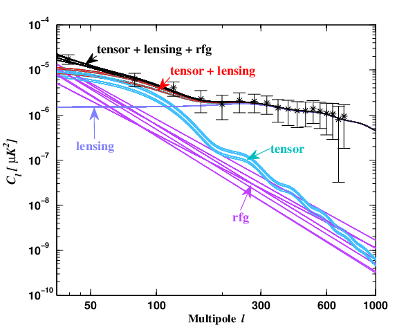
To show the above points more clearly, we plot in Figure 7 the data together with the model curves. This ensemble of curves corresponds to models drawn from a converged MCMC chain. By comparing the ‘tensor’ BB curve with the residual foreground, ‘rfg’, curve, we see that the region that is most affected by the residual foreground component coincides with the region where most of the gravity wave signal is present, at . This plot also illustrates the importance of measuring the B-mode power spectrum at in order to be able to estimate and subtract off the B-mode spectrum from lensing.
4.2 Effect of off-diagonal terms in the covariance matrix
Up to this point we were using a covariance matrix in which small off-diagonal components from the modelled residual foregrounds are ignored. In this section we address the question of how incorporating such off-diagonal terms in the covariance matrix affect our results.

The expression that combines all propagated uncertainties starting from component separation to power spectrum estimation is given by Eq. (8). The full covariance matrix for the bbasic and gtemplate cases is shown in Figure 1. We note that off-diagonal terms in both cases are several orders of magnitudes smaller than the diagonal elements.
In Figure 8 we compare the recovered values of our seven base parameters using diagonal (bbasic and gtemplate) and full covariance matrix (bbasic full cov and gtemplate full cov). For these cases, the effect of ignoring off-diagonal terms is small, with the shift on being slightly bigger in the gtemplate case. This is because, as shown in Figure 1, the residual foreground level is higher for this case. We conclude that at least for these cases, where the off-diagonal terms are small as compared to the diagonal ones, ignoring the off-diagonal terms has little impact on our results.
5 Conclusions
Foreground cleaning and the propagation of uncertainties related to this process is one of the outstanding issues in CMB data analysis for ongoing and future experiments. This is particularly important for CMB polarization measurements and the search for B-modes, for which foregrounds are expected to be sizeable at all frequencies and across most of the sky.
Based on the foreground cleaning procedure presented in [13], we developed and completed recent results from [12] concerning the propagation of foreground cleaning uncertainties in the main steps of CMB data analysis, with a focus on measuring the tensor to scalar ratio of cosmological perturbations. We considered typical experimental setups for proposed ground-based and balloon-borne experiments, for which the foreground contrast might be weak enough to justify the assumption of a spatially constant spectral index built into our parametric method.
These experiments operate at frequencies between 90 and 410 GHz, where the main diffuse foreground components are polarized synchrotron and thermal dust emission. We examined configurations in which a significant source of bias remains after the foreground cleaning phase, due to residual synchrotron emission from lower frequencies. In this case, we introduced a method for correcting the data for the presence of such a residual, simply by parametrizing the residual foreground power at low , and then marginalizing over its amplitude and powerlaw index. We found that this technique debiases the measurement, although in the case we studied the foreground parameters are poorly constrained, degrading the detection significance.
We characterize the error covariance due to subtracted foregrounds, and find it to be subdominant compared to instrumental noise and sample variance in our simulated data analysis.
We conclude that for the experimental configurations and template-based simulated foreground signals investigated here, it is possible to propagate foreground subtraction uncertainties and marginalize over foreground residuals, without biasing the final parameter determination results. Therefore, the expected performance of these multi-frequency experiments, usually quoted in the absence of a properly simulated data analysis procedure, might only be marginally degraded by the presence of foreground uncertainties and residuals.
Acknowledgments
YF thanks APC for hospitality while part of this project was completed. His work there was supported in part by French National Research Agency (ANR) through COSINUS program (project MIDAS no. ANR-09-COSI-009). Some of the results in this paper have been derived using the HEALPix [49] package. We acknowledge the use of CAMB [16] and CosmoMC [39] packages.
References
- (1) A. R. Liddle and D. H. Lyth, Cosmological Inflation and Large-Scale Structure. Cambridge University Press, Apr., 2000.
- (2) S. Dodelson, Modern cosmology. Academic Press, 2003.
- (3) M. Kamionkowski, A. Kosowsky and A. Stebbins, Statistics of cosmic microwave background polarization, Phys. Rev. D. 55 (June, 1997) 7368–7388 [arXiv:astro-ph/9611125].
- (4) U. Seljak and M. Zaldarriaga, Signature of Gravity Waves in the Polarization of the Microwave Background, Physical Review Letters 78 (Mar., 1997) 2054–2057 [arXiv:astro-ph/9609169].
- (5) U. Seljak and M. Zaldarriaga, Polarization of Microwave Background: Statistical and Physical Properties, ArXiv Astrophysics e-prints (May, 1998) [arXiv:astro-ph/9805010].
- (6) WMAP Collaboration, L. Page et. al., Three year Wilkinson Microwave Anisotropy Probe (WMAP) observations: Polarization analysis, Astrophys. J. Suppl. 170 (2007) 335 [astro-ph/0603450].
- (7) B. Gold, C. L. Bennett, R. S. Hill, G. Hinshaw, N. Odegard, L. Page, D. N. Spergel and et. al., Five-Year Wilkinson Microwave Anisotropy Probe Observations: Galactic Foreground Emission, ApJS 180 (Feb., 2009) 265–282 [0803.0715].
- (8) E. Komatsu, K. M. Smith, J. Dunkley, C. L. Bennett, B. Gold, G. Hinshaw, N. Jarosik, D. Larson, M. R. Nolta, L. Page, D. N. Spergel, M. Halpern, R. S. Hill, A. Kogut, M. Limon, S. S. Meyer, N. Odegard, G. S. Tucker, J. L. Weiland, E. Wollack and E. L. Wright, Seven-year Wilkinson Microwave Anisotropy Probe (WMAP) Observations: Cosmological Interpretation, ApJS 192 (Feb., 2011) 18–+ [1001.4538].
- (9) M. Amarie, C. Hirata and U. Seljak, Detectability of tensor modes in the presence of foregrounds, Phys. Rev. D. 72 (Dec., 2005) 123006–+ [arXiv:astro-ph/0508293].
- (10) G. Efstathiou, S. Gratton and F. Paci, Impact of Galactic polarized emission on B-mode detection at low multipoles, MNRAS 397 (Aug., 2009) 1355–1373 [0902.4803].
- (11) M. Betoule, E. Pierpaoli, J. Delabrouille, M. Le Jeune and J. Cardoso, Measuring the tensor to scalar ratio from CMB B-modes in the presence of foregrounds, A&A 503 (Sept., 2009) 691–706 [0901.1056].
- (12) F. Stivoli, J. Grain, S. M. Leach, M. Tristram, C. Baccigalupi and R. Stompor, Maximum likelihood, parametric component separation and CMB B-mode detection in suborbital experiments, MNRAS 408 (Nov., 2010) 2319–2335 [1004.4756].
- (13) R. Stompor, S. Leach, F. Stivoli and C. Baccigalupi, Maximum likelihood algorithm for parametric component separation in cosmic microwave background experiments, MNRAS 392 (Jan., 2009) 216–232 [0804.2645].
- (14) J. Grain, M. Tristram and R. Stompor, Polarized CMB power spectrum estimation using the pure pseudo-cross-spectrum approach, Phys. Rev. D. 79 (June, 2009) 123515–+ [0903.2350].
- (15) J. Dunkley, E. Komatsu, M. R. Nolta, D. N. Spergel, D. Larson, G. Hinshaw, L. Page, C. L. Bennett, B. Gold, N. Jarosik, J. L. Weiland, M. Halpern, R. S. Hill, A. Kogut, M. Limon, S. S. Meyer, G. S. Tucker, E. Wollack and E. L. Wright, Five-Year Wilkinson Microwave Anisotropy Probe Observations: Likelihoods and Parameters from the WMAP Data, ApJS 180 (Feb., 2009) 306–329 [0803.0586].
- (16) A. Lewis, A. Challinor and A. Lasenby, Efficient computation of CMB anisotropies in closed FRW models, Astrophys. J. 538 (2000) 473–476 [astro-ph/9911177].
- (17) E. F. Bunn, M. Zaldarriaga, M. Tegmark and A. de Oliveira-Costa, E/B decomposition of finite pixelized CMB maps, Phys. Rev. D. 67 (Jan., 2003) 023501–+ [arXiv:astro-ph/0207338].
- (18) K. M. Smith and M. Zaldarriaga, General solution to the E-B mixing problem, Phys. Rev. D. 76 (Aug., 2007) 043001–+ [arXiv:astro-ph/0610059].
- (19) K. M. Smith, Pure pseudo- estimators for CMB B-modes, New Astron.Rev 50 (Dec., 2006) 1025–1029 [arXiv:astro-ph/0608662].
- (20) M. Tristram, J. F. Macías-Pérez, C. Renault and D. Santos, XSPECT, estimation of the angular power spectrum by computing cross-power spectra with analytical error bars, MNRAS 358 (Apr., 2005) 833–842 [arXiv:astro-ph/0405575].
- (21) I. O. Hupca, J. Falcou, L. Grigori and R. Stompor, Spherical harmonic transform with GPUs, ArXiv e-prints (Oct., 2010) [1010.1260].
- (22) A. T. Lee, H. Tran, P. Ade, K. Arnold, J. Borrill, M. A. Dobbs, J. Errard, N. Halverson, W. L. Holzapfel and et. al., POLARBEAR: Ultra-high Energy Physics with Measurements of CMB Polarization, in American Institute of Physics Conference Series (H. Kodama & K. Ioka, ed.), vol. 1040 of American Institute of Physics Conference Series, pp. 66–77, Aug., 2008.
- (23) B. Reichborn-Kjennerud, A. M. Aboobaker, P. Ade, F. Aubin, C. Baccigalupi, C. Bao, J. Borrill, C. Cantalupo, D. Chapman, J. Didier, M. Dobbs, J. Grain, W. Grainger, S. Hanany and et al, EBEX: a balloon-borne CMB polarization experiment, in Society of Photo-Optical Instrumentation Engineers (SPIE) Conference Series, vol. 7741, July, 2010. 1007.3672.
- (24) D. T. O’Dea, P. A. R. Ade, M. Amiri, S. J. Benton, J. J. Bock, J. R. Bond, J. A. Bonetti, S. Bryan, B. Burger, H. C. Chiang, C. N. Clark, C. R. Contaldi, B. P. Crill, G. Davis, O. Dore, M. Farhang, J. P. Filippini, L. M. Fissel, A. A. Fraisse, N. N. Gandilo, S. Golwala, J. E. Gudmundsson, M. Hasselfield, G. Hilton, W. Holmes, V. V. Hristov, K. Irwin, W. C. Jones, C. L. Kuo, C. J. MacTavish, P. V. Mason, T. E. Montroy, T. A. Morford, C. B. Netterfield, A. S. Rahlin, C. Reintsema, J. E. Ruhl, M. C. Runyan, M. A. Schenker, J. A. Shariff, J. D. Soler, A. Trangsrud, C. Tucker, R. S. Tucker, A. D. Turner and D. Wiebe, Spider Optimization II: Optical, Magnetic and Foreground Effects, ArXiv e-prints (Feb., 2011) [1102.0559].
- (25) T. E. Montroy, P. A. R. Ade, J. J. Bock, J. R. Bond, J. Borrill, A. Boscaleri, P. Cabella, C. R. Contaldi, B. P. Crill, P. de Bernardis, A. De Gasperis, G.and de Oliveira-Costa and et. al., A Measurement of the CMB Spectrum from the 2003 Flight of BOOMERANG, ApJ 647 (Aug., 2006) 813–822 [arXiv:astro-ph/0507514].
- (26) H. C. Chiang, P. A. R. Ade, D. Barkats, J. O. Battle, E. M. Bierman, J. J. Bock, C. D. Dowell, L. Duband, E. F. Hivon, W. L. Holzapfel, V. V. Hristov, W. C. Jones and et. al., Measurement of Cosmic Microwave Background Polarization Power Spectra from Two Years of BICEP Data, ApJ 711 (Mar., 2010) 1123–1140 [0906.1181].
- (27) M. Lueker, C. L. Reichardt, K. K. Schaffer, O. Zahn, P. A. R. Ade, K. A. Aird, B. A. Benson, L. E. Bleem, J. E. Carlstrom, C. L. Chang, H. Cho, T. M. Crawford, A. T. Crites and et. al., Measurements of Secondary Cosmic Microwave Background Anisotropies with the South Pole Telescope, ApJ 719 (Aug., 2010) 1045–1066 [0912.4317].
- (28) M. L. Brown, P. Ade, J. Bock, M. Bowden, G. Cahill, P. G. Castro, S. Church, T. Culverhouse, R. B. Friedman, K. Ganga, W. K. Gear, S. Gupta, et. al. and The QUa D collaboration, Improved Measurements of the Temperature and Polarization of the Cosmic Microwave Background from QUaD, ApJ 705 (Nov., 2009) 978–999 [0906.1003].
- (29) C. L. Reichardt, P. A. R. Ade, J. J. Bock, J. R. Bond, J. A. Brevik, C. R. Contaldi, M. D. Daub, J. T. Dempsey and et. al., High-Resolution CMB Power Spectrum from the Complete ACBAR Data Set, ApJ 694 (Apr., 2009) 1200–1219 [0801.1491].
- (30) C. Bischoff, A. Brizius, I. Buder, Y. Chinone, K. Cleary, R. N. Dumoulin, A. Kusaka, R. Monsalve, S. K. Naess, L. B. Newburgh, R. Reeves, K. M. Smith, I. K. Wehus, J. A. Zuntz, J. T. L. Zwart, L. Bronfman, R. Bustos, S. E. Church and et al ArXiv e-prints (Dec., 2010) [1012.3191].
- (31) G. Haslam, R. Wielebinski and W. Priester, Radio maps of the sky, SKYTEL 63 (Mar., 1982) 230–232.
- (32) D. P. Finkbeiner, M. Davis and D. J. Schlegel, Extrapolation of Galactic Dust Emission at 100 Microns to Cosmic Microwave Background Radiation Frequencies Using FIRAS, ApJ 524 (Oct., 1999) 867–886 [arXiv:astro-ph/9905128].
- (33) G. Giardino, A. J. Banday, K. M. Górski, K. Bennett, J. L. Jonas and J. Tauber, Towards a model of full-sky Galactic synchrotron intensity and linear polarisation: A re-analysis of the Parkes data, A&A 387 (May, 2002) 82–97 [arXiv:astro-ph/0202520].
- (34) H. K. Eriksen, C. Dickinson, C. R. Lawrence, C. Baccigalupi, A. J. Banday, K. M. Górski, F. K. Hansen, P. B. Lilje, E. Pierpaoli, M. D. Seiffert, K. M. Smith and K. Vanderlinde, Cosmic Microwave Background Component Separation by Parameter Estimation, ApJ 641 (Apr., 2006) 665–682 [arXiv:astro-ph/0508268].
- (35) V. Stolyarov, M. P. Hobson, A. N. Lasenby and R. B. Barreiro, All-sky component separation in the presence of anisotropic noise and dust temperature variations, MNRAS 357 (Feb., 2005) 145–155 [arXiv:astro-ph/0405494].
- (36) M. Tucci, E. Martínez-González, P. Vielva and J. Delabrouille, Limits on the detectability of the CMB B-mode polarization imposed by foregrounds, MNRAS 360 (July, 2005) 935–949 [arXiv:astro-ph/0411567].
- (37) L. Verde, H. V. Peiris and R. Jimenez, Considerations in optimizing CMB polarization experiments to constrain inflationary physics, J. Cosmology Astropart. Phys. 1 (Jan., 2006) 19–+ [arXiv:astro-ph/0506036].
- (38) J. R. Bond, A. H. Jaffe and L. Knox, Radical Compression of Cosmic Microwave Background Data, ApJ 533 (Apr., 2000) 19–37 [arXiv:astro-ph/9808264].
- (39) A. Lewis and S. Bridle, Cosmological parameters from CMB and other data: A Monte Carlo approach, Phys. Rev. D. 66 (Nov., 2002) 103511–+ [arXiv:astro-ph/0205436].
- (40) Planck Collaboration, P. A. R. Ade, N. Aghanim, M. Arnaud, M. Ashdown, J. Aumont, C. Baccigalupi, M. Baker, A. Balbi, A. J. Banday and et al., Planck Early Results: The Planck mission, ArXiv e-prints (Jan., 2011) [1101.2022].
- (41) L. Perotto, J. Lesgourgues, S. Hannestad, H. Tu and Y. Y Y Wong, Probing cosmological parameters with the CMB: forecasts from Monte Carlo simulations, Journal of Cosmology and Astro-Particle Physics 10 (Oct., 2006) 13–+ [arXiv:astro-ph/0606227].
- (42) N. Jarosik, C. L. Bennett, J. Dunkley, B. Gold, M. R. Greason, M. Halpern, R. S. Hill, G. Hinshaw, A. Kogut, E. Komatsu, D. Larson, M. Limon, S. S. Meyer, M. R. Nolta, N. Odegard, L. Page, K. M. Smith, D. N. Spergel, G. S. Tucker, J. L. Weiland, E. Wollack and E. L. Wright, Seven-year Wilkinson Microwave Anisotropy Probe (WMAP) Observations: Sky Maps, Systematic Errors, and Basic Results, ApJS 192 (Feb., 2011) 14–+ [1001.4744].
- (43) A. Lewis, Lensed CMB simulation and parameter estimation, Phys. Rev. D. 71 (Apr., 2005) 083008–+ [arXiv:astro-ph/0502469].
- (44) N. Katayama and E. Komatsu, Simple foreground cleaning algorithm for detecting primordial B-mode polarization of the cosmic microwave background, ArXiv e-prints (Jan., 2011) [1101.5210].
- (45) A. Bonaldi and S. Ricciardi, Forecast B-modes detection at large scales in presence of noise and foregrounds, ArXiv e-prints (Jan., 2011) [1101.4876].
- (46) C. Armitage-Caplan, J. Dunkley, H. K. Eriksen and C. Dickinson, Large-Scale Polarized Foreground Component Separation for Planck, ArXiv e-prints (Mar., 2011) [1103.2554].
- (47) G. Hinshaw, D. N. Spergel, L. Verde, R. S. Hill, S. S. Meyer, C. Barnes, C. L. Bennett, M. Halpern, N. Jarosik, A. Kogut, E. Komatsu, M. Limon, L. Page, G. S. Tucker, J. L. Weiland, E. Wollack and E. L. Wright, First-Year Wilkinson Microwave Anisotropy Probe (WMAP) Observations: The Angular Power Spectrum, ApJS 148 (Sept., 2003) 135–159 [arXiv:astro-ph/0302217].
- (48) D. N. Spergel, R. Bean, O. Doré, M. R. Nolta, C. L. Bennett, J. Dunkley, G. Hinshaw, N. Jarosik, E. Komatsu, L. Page, H. V. Peiris, L. Verde, M. Halpern, R. S. Hill, A. Kogut, M. Limon, S. S. Meyer, N. Odegard, G. S. Tucker, J. L. Weiland, E. Wollack and E. L. Wright, Three-Year Wilkinson Microwave Anisotropy Probe (WMAP) Observations: Implications for Cosmology, ApJS 170 (June, 2007) 377–408 [arXiv:astro-ph/0603449].
- (49) K. M. Górski, E. Hivon, A. J. Banday, B. D. Wandelt, F. K. Hansen, M. Reinecke and M. Bartelmann, HEALPix: A Framework for High-Resolution Discretization and Fast Analysis of Data Distributed on the Sphere, ApJ 622 (Apr., 2005) 759–771 [arXiv:astro-ph/0409513].