Width of the longitudinal magnon in the vicinity of the O(3) quantum critical point
Abstract
We consider a three-dimensional quantum antiferromagnet in the vicinity of a quantum critical point separating the magnetically ordered and the magnetically disordered phases. A specific example is TlCuCl3 where the quantum phase transition can be driven by hydrostatic pressure and/or by external magnetic field. As expected two transverse and one longitudinal magnetic excitation have been observed in the pressure driven magnetically ordered phase. According to the experimental data, the longitudinal magnon has a substantial width, which has not been understood and has remained a puzzle. In the present work, we explain the mechanism for the width, calculate the width and relate value of the width with parameters of the Bose condensate of magnons observed in the same compound. The method of an effective quantum field theory is employed in the work.
pacs
64.70.Tg, 75.10.Jm, 75.40.GbI Introduction
Continuous Quantum Phase Transitions (QPT) and behaviour of quantum systems in vicinity of the corresponding quantum critical points attract a great research interest[1] both in theory and in experiment. There are manifestations of such effects in cuprate superconductors, in iron pnictides and in other materials. QPT are most pronounced in low dimensional systems, but they also occur in three dimensional (3D) systems. In the present paper we consider quantum systems, therefore 3D means 3D+time. A well known material that manifests the 3D magnetic quantum critical behaviour is TlCuCl3. Magnetic and other properties of the compound has been extensively studied experimentally. [2, 3, 4, 5, 6, 7, 8, 9, 10, 11, 12, 13, 14] Under normal conditions the material is nonmagnetic, while a magnetic field and/or pressure drives a QPT to the magnetically ordered phase. An analogous material KCuCl3 have similar properties. [15, 16] It has been understood that TlCuCl3 consists of a 3D set of spin dimers and the QPT in the magnetic field can be considered as Bose condensation of the spin dimer triplet excitations (triplons). [17, 18, 19, 20, 21, 22, 1] The pressure induced QPT can be also described in terms of triplons.[23] Inelastic neutron scattering from the magnetically ordered phase in the vicinity of the pressure induced QPT [10] clearly indicates two transverse and one longitudinal spin-wave excitation modes as one would expect for condensed triplons. According to the data [10] the longitudinal spin-wave excitation has a finite width. Generically this is also expected because of the possibility for the longitudinal mode to decay to two transverse spin-wave excitations. However to the best of our knowledge this width has never been calculated. In the present work we perform such a calculation and compare the result with the experimental data. The width is related to theparameters of the Bose condensate of magnons observed in the same compound in the external magnetic field. On the technical side in the present work we use the effective quantum field theory approach.
As we pointed out, a description of the system in terms of the spin dimer triplon technique is also possible. The spin dimer technique accounts for both the short range and the long range dynamics on equal footing. On the one hand, this is a strength of this description. On the other hand, the description is quite technically involved if one needs to analyze the interaction effects that we are after. The technical complexity is a price for the universality. The effective quantum field theory method adopted in the present work, allows us to account for the interaction effects much more accurately. The method does not account for the short range dynamics, but the short range effects are irrelevant in the vicinity of a QPT.
We would like also to note that in the present paper we use terms “spin waves” and “magnons” on equal footing, having in mind magnetic excitations on both sides of the QPT.
II Effective field theory
The QPT that we consider here is a continuous zero temperature transition. Therefore, the short range dynamics are not changed in the QPT, only the long range dynamics are changed. In this situation it is quite natural to apply the effective field theory approach to describe the transition [24]. A similar approach was used to analyse the longitudinal mode in a quasi-one dimensional antiferromagnet.[25] Technically this approach is much simpler than the triplon description. The effective field theory must be written in terms of the vector field that describes staggered magnetization as well as the long-wave-length magnetic excitations. There is no net magnetization on both sides of the QPT, only the staggered magnetization, hence the effective Landau-Ginzburg Lagrangian corresponding to the nonlinear -model describes the system,
We note the standard logic for this effective Lagrangian. (i) The elastic energy must be proportional to (stiffness). (ii) The system consists of spins with the same gyromagnetic ratio . Therefore the Larmor theorem must be valid: If there is a state of the system without magnetic field, then the same state in a uniform magnetic field must precess with frequency (Hereafter we set , where is Bohr magneton.) (iii) The static energy can depend on the magnetic field only quadratically because the system has no net magnetization. Note that instead of the hard constraint, , usually used in the nonlinear -model, we impose the “soft” quartic interaction . The QPT is due to the mass term,
| (2) |
In TlCuCl3 the QPT is driven by external hydrostatic pressure and this is reflected in Eq.(2), is just a coefficient. In a more general situation pressure has to be replaced by a generalized “coupling constant”. When and there is no magnetic field, , the mass squared is positive and this corresponds to the magnetically disordered phase with the gapped triple degenerate spin-wave dispersion . When the mass squared is negative and this results in a nonzero expectation value of that describes the spontaneous antiferromagnetic ordering with a gapped longitudinal mode and two gapless Goldstone modes.
III Spin-wave dispersion in TlCuCl3 at zero pressure
Since we will compare our results with experimental data for TlCuCl3 we need to determine the corresponding spin-wave velocity . TlCuCl3 has a monoclinic structure [2] with a unit cell very close to a rectangular prism with lattice parameters , , and an angle only slightly deviating from a right angle (). The spin wave dispersion over the Brillouin zone was determined by inelastic neutron scattering and the dispersion can be very well fit by the following formula [17, 22]
| (3) | |||
Here , are dimensionless momenta. The dispersion has minimum at . Near the minimum the dispersion squared can be expanded in powers of momentum, , where , , , and the coefficients are expressed in terms of parameters from (3). Diagonalization of the quadratic form gives the spin-wave velocities ,
| (4) | |||
The expansion (4) is generally valid only at small momenta, , however, accidentally the simple quadratic dependence along the “softest” direction is valid practically up to the boundary of the Brillouine zone, . Therefore, magnetism in TlCuCl3 is three-dimensional up to the energy/temperature above the gap. At a higher energy/temperature the magnetism becomes two-dimensional.
IV Spin-wave excitations at zero temperature and zero magnetic field
Taking into account Eq.(4) the stiffness term in the effective action (II) has to be replaced by
| (5) |
In the magnetically disordered phase, the Lagrangian (II) yields the following triple degenerate spectrum
| (6) | |||||
Comparing with the gap measured in neutron scattering, Ref. [10], and presented in Fig. 1 by blue triangles we determine the value of , . Here we take into account that .

The experimental data [10] presented in Fig. 1 demonstrate some anisotropy that is not accounted in the Lagrangian (II). At the moment we disregard the anisotropy and return to this point later. On the other side of the QPT, , the field attains spontaneously the following expectation value
| (7) |
The subscript “c” in stands for classical expectation value. We chose the classical field to be directed along the z-axis in the spin space. Further standard analysis of the effective Lagrangian shows that there are two transverse gapless Goldstone x- and y-modes
| (8) |
and one gapped longitudinal z-mode with dispersion
| (9) | |||||
The “longitudinal” gap agrees pretty well with the data shown in Fig. 1 by red triangles and diamonds.
V Bose condensation in magnetic field and the quartic term in the Lagrangian
To calculate the width of the longitudinal spin wave we need to know the coefficient in the quartic term in (II). To determine the coefficient we turn to the analysis of Bose condensation of magnons in the external magnetic field at zero pressure. The Lagrangian (II) results in the following energy density
| (10) | |||||
Here since . In the energy we skip all terms with derivatives since we are interested in Bose condensation in a homogeneous system. For magnetic field , the energy is minimized when , there is no spontaneous magnetization. For magnetic field (i.e. when the gap is closed), the energy is minimum when
| (11) |
Thus, there is a spontaneous staggered magnetization perpendicular to the direction of the magnetic field. The magnetization can be arbitrarily rotated around the direction of the magnetic field, therefore, the system retains a U(1) symmetry as it should be for a Bose condensate. Substitution of the expectation value (11) back to Eq.(10) gives the following energy density of the condensate
| (12) |
In the second equality in this equation we assume that , i.e. we are close to the phase transition point at . This concludes the analysis of Bose condensation in terms of the effective action.
It is well known that the Bose condensation of magnons can be also analysed in terms of usual Schrodinger equation within the Hartree-Fock-Popov approximation. Such an analysis has been performed earlier in Ref. 22. In the Hartree-Fock-Popov approximation the density energy of the condensate at zero temperature reads
| (13) |
where is the condensate density and is the effective repulsion between magnons. The arrow “” shows the result of the energy minimization with respect to . Comparing (12) and (13) we express the field theory parameter is terms of the Hartree-Fock-Popov parameter , . Fit of data [4] for Bose condensation in TlCuCl3 performed in Ref. 22 gave the value of the effective repulsion, . The data in Ref. 4 is taken at zero pressure, therefore . All in all we get
| (14) |
According to the fit in Ref. 22, there is a margin of error of about 20% in the values of and .
VI Width of the longitudinal magnon

Decay of the longitudinal magnon is due to the quartic term in (II) and is described by the diagram shown in Fig. 2. To calculate the decay amplitude one needs first to rewrite the Lagrangian in terms of magnons in the magnetically ordered phase. After substitution of in Eq.(II) (the condensate field is given by Eq.(7)) we find the quadratic and the cubic part of the Lagrangian
| (15) | |||||
The stiffness term is determined in Eq.(5). Standard quantization of the quadratic Lagrangian gives (we set )
where and are corresponding annihilation and creation operators. The decay matrix element shown in Fig. 2 is determined after the operators (VI) are substituted in the cubic Lagrangian ,
| (16) |
where is the momentum of the initial longitudinal magnon and , are the momenta of the final transverse magnons. The coefficient 2 in (16) is due to two different ways for pairing of creation and annihilation operators. The decay width is given by Fermi golden rule
| (17) | |||||
where the coefficient stands to avoid the double counting of final bosonic states. Integration in (17) is straightforward, the answer is
| (18) |
In this equation are the components of the vector .
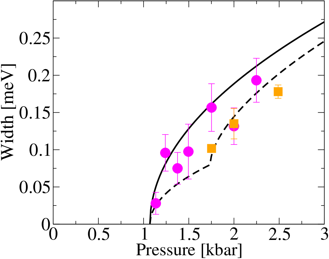
According to (18) the width in a reasonable agreement with experimental data from Ref.10 presented in Fig.3. According to Eqs. (18),(4),(14) the theoretical value for the ratio is . The corresponding theoretical curve for versus pressure is shown in Fig. 3 by the black solid line together with experimental data [10] shown in the same figure. We stress that we calculate not only the functional dependence of the gap on the pressure. We calculate the absolute value of the gap. Overall the agreement between the theory and the experiment is quite good having in mind experimental error bars, Fig.3, as well as 20% theoretical uncertainty in the value of . The agreement can be further improved if one accounts for the spin-orbit anisotropy. We discuss the anisotropy in the next section.
VII Account for anisotropy induced by the spin-orbit interaction
Data presented in Fig.1 clearly indicate an easy plane anisotropy in the magnetically ordered phase: one of the transverse magnons is gapped with the constant gap
| (19) |
where the subscript “a” stands for anisotropy. To incorporate the anisotropy in our description we have to add the term
| (20) |
to the effective Lagrangian (II). With account of the anisotropy the triple degeneracy of the dispersion in the magnetically disordered phase, , is lifted, the z- and y-modes have the same dispersion (6) as before while the x-mode has a higher energy
The corresponding gaps () are plotted by lines in Fig.1 versus pressure. The dispersion in the magnetically ordered phase, , is the following
| (21) | |||||
The corresponding gaps () are also plotted by lines in Fig.1 versus pressure. Overall agreement between the theory and the experimental data presented in the same Fig.1 is excellent.
The anisotropy gap influences the width of the longitudinal magnon only via limitation of the decay phase space. A straightforward calculation shows that Eq.(18) has to be modified in the following way
| (22) |
Here is the step function, if , otherwise . The calculated decay width is shown in Fig.3 by the dashed line. The agreement with experiment is excellent.
VIII conclusions
The decay width of the longitudinal magnon in the vicinity of the O(3) quantum critical point of a three-dimensional quantum antiferromagnet has been calculated using the effective field theory approach. The results are quite generic.
We also compared our results with experimental data for TlCuCl3 where the quantum phase transition can be driven by hydrostatic pressure and/or by external magnetic field. The parameters of the effective action were determined from available data for inelastic neutron scattering and for Bose condensation of magnons in the external magnetic field. Having determined these parameters, we calculated the decay width. The result agrees very well with measurements.
IX acknowledgement
We are grateful to B. Normand for stimulating discussions and to J. Oitmaa for important comments.
References
- [1] S. Sachdev and B. Keimer, Phys. Today 64, February, 29 (2011).
- [2] K. Takatsu, W. Shiramura and H. Tanaka, J. Phys. Soc. Jpn., 66, 1611 (1997).
- [3] A. Oosawa, M. Ishii, and H. Tanaka, J. Phys. Cond. Mat., 11 , 265 (1999).
- [4] T. Nikuni, M. Oshikawa, A. Oosawa, and H. Tanaka, Phys. Rev. Lett., 84 , 5868 (2000).
- [5] N. Cavadini, G. Heigold, W. Henggeler, A. Furrer, H.-U. G�del, K. Kr�mer, and H. Mutka, Phys. Rev. B 63, 172414 (2001).
- [6] K.-Y. Choi, G. Guntherodt, A. Oosawa, H. Tanaka, and P. Lemmens, Phys. Rev. B 68, 174412 (2003).
- [7] E. Ya. Sherman, P. Lemmens, B. Busse, A. Oosawa, and H. Tanaka, Phys. Rev. Lett., 91, 057201 (2003).
- [8] V. N. Glazkov, A. I. Smirnov, H. Tanaka, and A. Oosawa, Phys. Rev. B 69, 184410 (2004).
- [9] Ch. Rüegg, A. Furrer, D. Sheptyakov, Th. Strässle, K. W. Krämer, H.-U. Güdel, and L. Mélési, Phys. Rev. Lett. 93, 257201 (2004).
- [10] Ch. Rüegg, B. Normand, M. Matsumoto, A. Furrer, D. F. McMorrow, K. W. Krämer, H.-U. Güdel, S. N. Gvasaliya, H. Mutka, and M. Boehm, Phys. Rev. Lett. 100, 205701 (2008).
- [11] K. Goto, N. Fujisawa, T. Ono, H. Tanaka, and Y. Uwatoko, J. Phys. Soc. Jpn. 73, 3254 (2004).
- [12] K. Goto, T. Ono, H. Tanaka, A. Oosawa, Y. Uwatoko, K. Kakurai, and T. Osakabe, AIP Conf. Proc. 850, 1059 (2006).
- [13] H. Tanaka, F. Yamada, T. Ono, T. Sakakibara, Y. Uwatoko, A. Oosawa, K. Kakurai, and K. Goto, J. Magn. Magn. Mater. 310, 1343 (2007).
- [14] F. Yamada, Y. Ishii, T. Suzuki, T. Matsuzaki, and H. Tanaka, Phys. Rev. B 78, 224405 (2008).
- [15] T. Sakurai, A. Taketani, S. Kimura, M. Yoshida, S. Okubo, H. Ohta, H. Tanaka, and Y. Uwatoko, AIP Conf. Proc. 850, 1057 (2006).
- [16] K. Goto, T. Osakabe, K. Kakurai, Y. Uwatoko, A. Oosawa, J. Kawakami, and H. Tanaka, J. Phys. Soc. Jpn. 76, 053704 (2007).
- [17] M. Matsumoto, B. Normand, T. M. Rice, and M. Sigrist, Phys. Rev. Lett., 89, 077203 (2002).
- [18] M. Matsumoto, B. Normand, T. M. Rice, and M. Sigrist, Phys. Rev. B 69, 054423 (2004).
- [19] G. Misguich and M. Oshikawa, J. Phys. Soc. Jpn. 73, 3429 (2004).
- [20] J. Sirker, A. Weisse and O. P. Sushkov, Europhys. Lett., 68, 275 (2004).
- [21] J. Sirker, A. Weisse and O. P. Sushkov, Physica B 359, 1318 (2005).
- [22] J. Sirker, A. Weisse and O. P. Sushkov, J. Phys. Soc. Jpn. 74, 129 (Suppl) (2005).
- [23] B. Normand, M. Matsumoto, O. Nohadani, S. Wessel, S. Haas, T. M. Rice, and M. Sigrist, J. Phys.: Condens. Matter 16, S867 (2004).
- [24] S. Sachdev, arXive:0910.1139, Contributed chapter to the book ”Understanding Quantum Phase Transitions,” edited by Lincoln D. Carr (Taylor & Francis, Boca Raton, 2010).
- [25] I. Affleck and G. F. Wellman, Phys. Rev. B 46, 8934 (1992).