跳到论文正文
W Papers独立论文阅读器 arXiv:1104.1057 论文正文 计算阅读时间 · 0%
引用这篇论文根据当前论文元数据生成,正式投稿前建议核对。


License: arXiv.org perpetual non-exclusive license
arXiv:1104.1057v1 [cs.IT] 06 Apr 2011

Bounds on the Capacity of the Relay Channel with Noncausal State at Source

Abdellatif Zaidi   Shlomo Shamai (Shitz)   Pablo Piantanida   Luc Vandendorpe ††thanks: Abdellatif Zaidi is with Université Paris-Est Marne La Vallée, 77454 Marne la Vallée Cedex 2, France. Email: abdellatif.zaidi@univ-mlv.fr††thanks: Shlomo Shamai is with the Department of Electrical Engineering, Technion Institute of Technology, Technion City, Haifa 32000, Israel. Email: sshlomo@ee.technion.ac.il††thanks: Pablo Piantanida is with the Department of Telecommunications, SUPELEC, 91190 Gif-sur-Yvette, France. Email: pablo.piantanida@supelec.fr††thanks: Luc Vandendorpe is with École Polytechnique de Louvain, Université Catholique de Louvain, Louvain-la-Neuve 1348, Belgium. Email: luc.vandendorpe@uclouvain.be††thanks: This work has been supported by the European Commission in the framework of the FP7 Network of Excellence in Wireless Communications (NEWCOM++). The work of S. Shamai has also been supported by the CORNET consortium.
Abstract

We consider a three-terminal state-dependent relay channel with the channel state available non-causally at only the source. Such a model may be of interest for node cooperation in the framework of cognition, i.e., collaborative signal transmission involving cognitive and non-cognitive radios. We study the capacity of this communication model. One principal problem is caused by the relay’s not knowing the channel state. For the discrete memoryless (DM) model, we establish two lower bounds and an upper bound on channel capacity. The first lower bound is obtained by a coding scheme in which the source describes the state of the channel to the relay and destination, which then exploit the gained description for a better communication of the source’s information message. The coding scheme for the second lower bound remedies the relay’s not knowing the states of the channel by first computing, at the source, the appropriate input that the relay would send had the relay known the states of the channel, and then transmitting this appropriate input to the relay. The relay simply guesses the sent input and sends it in the next block. The upper bound is non trivial and it accounts for not knowing the state at the relay and destination. For the general Gaussian model, we derive lower bounds on the channel capacity by exploiting ideas in the spirit of those we use for the DM model; and we show that these bounds are optimal for small and large noise at the relay irrespective to the strength of the interference. Furthermore, we also consider a special case model in which the source input has two components one of which is independent of the state. We establish a better upper bound for both DM and Gaussian cases and we also characterize the capacity in a number of special cases.

Index Terms: 
User cooperation, relay channel, cognitive radio, channel state information, dirty paper coding.

I Introduction

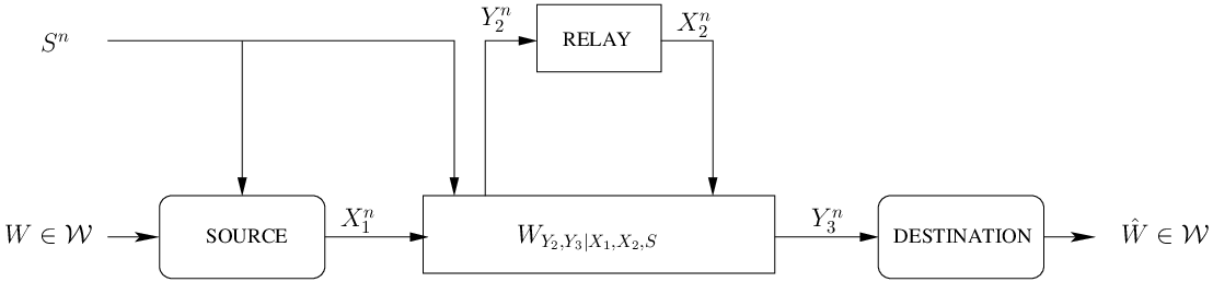
We consider a three-terminal state-dependent relay channel (RC) in which, as shown in Figure 1, the source wants to communicate a message WW to the destination through the state-dependent RC in nn uses of the channel, with the help of the relay. The channel outputs Y2nY^{n}_{2} and Y3nY^{n}_{3} for the relay and the destination, respectively, are controlled by the channel input X1nX^{n}_{1} from the source, the relay input X2nX^{n}_{2} and the channel state SnS^{n}, through a given memoryless probability law WY2,Y3|X1,X2,SW_{Y_{2},Y_{3}|X_{1},X_{2},S}. The channel state SnS^{n} is generated according to the nn-product of a given memoryless probability law QSQ_{S}. It is assumed that the channel state is known, noncausally, to only the source. The destination estimates the message sent by the source from the received channel output. In this paper we study the capacity of this communication system. We will refer to the model in Figure 1 as general state-dependent RC with informed source.
Refer to caption
Fig. 1: General state-dependent relay channel with state information SnS^{n} available non-causally at only the source.

We shall also study an important special case of the general model, shown in Figure 2. In this special model, the source alphabet 𝒳1=𝒳1​R×𝒳1​D\mathcal{X}_{1}=\mathcal{X}_{1R}\times\mathcal{X}_{1D}, X1n=(X1​Rn,X1​Dn)X^{n}_{1}=(X^{n}_{1R},X^{n}_{1D}) and only the component X1​DnX^{n}_{1D} knows the states SnS^{n}. Furthermore, the memoryless conditional law WY2,Y3|X1​R,X1​D,X2,SW_{Y_{2},Y_{3}|X_{1R},X_{1D},X_{2},S} factorizes as

WY2,Y3|X1​R,X1​D,X2,S=WY2|X1​R,S​WY3|X1​D,X2,S.W_{Y_{2},Y_{3}|X_{1R},X_{1D},X_{2},S}=W_{Y_{2}|X_{1R},S}W_{Y_{3}|X_{1D},X_{2},S}. (1)

One can think of the two source encoder components in Figure 2 as being two non-colocated base stations transmitting a common message to some destination with the help of a relay – the common message may be obtained by means of message cognition at the encoder whose input is heard at the relay.

Refer to caption
Fig. 2: State-dependent relay channel with the source input X1n=(X1​Rn,X1​Dn)X^{n}_{1}=(X^{n}_{1R},X^{n}_{1D}), and only the component X1​DnX^{n}_{1D} knowing the states of the channel non-causally.

I-A Background and Related Work

Channels whose probabilistic input-output relation depends on random parameters, or channel states, have spurred much interest and can model a large variety of problems, each related to some physical situation of interest. The random state sequence may be known in a causal or non-causal manner. For single user models, the concept of channel state available at only the transmitter dates back to Shannon [1] for the causal channel state case, and to Gel’fand and Pinsker [2] for the non-causal channel state case. In [3], Heegard and El Gamal study a model in which the state sequence is known non-causally to only the encoder or to only the decoder. They also derive achievable rates for the case in which partial channel state information (CSI) is given at varying rates to both the encoder and the decoder. In [4], Costa studies an additive Gaussian channel with additive Gaussian state known at only the encoder, and shows that Gel’fand-Pinsker coding with a specific auxiliary random variable, known as dirty paper coding (DPC), achieves the channel capacity. Interestingly, in this case, the DPC removes the effect of the additive channel state on the capacity as if there were no channel state present in the model or the channel state were known to the decoder as well. For a comprehensive review of state-dependent channels and related work, the reader may refer to [5].

A growing body of work studies multi-user state-dependent models. Recent advances in this regard can be found in [5, 6, 7, 8, 9, 10, 11, 12, 13, 14, 15, 16, 17, 18, 19, 20, 21, 22, 23, 24, 25, 26], and many other works. Key to the investigation of a state-dependent model is whether the parameters controlling the channel are known to all or only some of the users in the communication model. If the parameters of the channel are known to only some of the users, the problem exhibits some asymmetry which makes its investigation more difficult in general. Also, in this case one has to expect some rate penalty due to the lack of knowledge of the state at the uninformed encoders, relative to the case in which all encoders would be informed.

The state-dependent multiaccess channel (MAC) with only one informed encoder and degraded message sets is considered in [27, 28, 7, 29, 30, 6]; and the state-dependent relay channel (RC) with only informed relay is considered in [11, 12]. For all these models, the authors develop non-trivial outer or upper bounds that permit to characterize the rate loss due to not knowing the state at the uninformed encoders. Key feature to the development of these outer or upper bounding techniques is that, in all these models, the uninformed encoder not only does not know the channel state but can learn no information about it.

The model for the RC with informed source that we study in this paper seemingly exhibits some similarities with the RC with informed relay considered in [11, 12], and it also connects with the MAC with asymmetric channel state and degraded message sets considered in [7, 6, 8]. However, establishing a non-trivial upper bound for the present model is more involved, comparatively. Partly, this is because, here, one uninformed encoder (the relay) is also a receiver; and, so, it can potentially get some information about the channel states from directly observing the past received sequence from the source. That is, at time ii, the input X2,iX_{2,i} of the relay can potentially depend on the channel states through its past output Y2i−1=(Y2,1,…,Y2,i−1)Y_{2}^{i-1}=(Y_{2,1},\ldots,Y_{2,i-1}). For the general model in Figure 1, the relay can even know the states non-causally, potentially. This is because Y2i−1Y_{2}^{i-1} may depend on future values of the state through past source inputs X1,j​(W,Sn)X_{1,j}(W,S^{n}), j=1,…,i−1j=1,\ldots,i-1. For the special case in Figure 2, the relay can know the states only strictly-causally, but upper bounding the capacity seems still not easy. In our recent work [31, 32], we have shown that, in a multiaccess channel, strictly causal knowledge of the state at one encoder can be beneficial in general for the other encoder even if the latter is informed non-causally; but the capacity region is still to be characterized in general. Studying networks in which a subset of the nodes know the states non-causally and another subset know these states only strictly causally, i.e., networks with mixed – noncausal and strictly causal, states appears to be more challenging in general, and is likely to capture additional interest, especially after recent results on the utility of strictly causally known states in multiaccess channels [16, 17].

I-B Main Contributions

For the general state-dependent RC with informed source shown in Figure 1, we derive two lower bounds and an upper bound on the channel capacity. In the discrete memoryless (DM) case, the first lower bound is obtained by a block Markov coding scheme in which the source describes the channel state to the relay and destination ahead of time. The source sends a two-layer description of the state consisting of two (possibly correlated) individual descriptions intended to be recovered at the relay and destination respectively. The relay recovers the individual description intended to it and then utilizes the estimated state as non-causal state information at the transmitter to implement collaborative source-relay binning in subsequent blocks, through a combined decode-and-forward [33, Theorem 5] and Gel’fand-Pinsker binning [2]. The destination guesses the source’s message sent cooperatively by the source and relay and the individual description which is intended to it from its output and the previously recovered state. The rationale for the coding scheme which we use for the first lower bound is that, had the relay known the state with negligible distortion, then efficient cooperative source-relay binning in the spirit of [34] can be realized (recall that the model in [34] assumes availability of the state at both source and relay).

We obtain the second lower bound by a block Markov coding scheme in which, rather than the channel state itself, the source describes to the relay the appropriate input that the relay would send had the relay known the channel states, assuming a decode-and-forward relaying strategy. The source sends this description to the relay ahead of time. The relay recovers the sent input and retransmits it in the appropriate subsequent block. The rationale for the coding scheme which we use for the second lower bound is that, if the input is produced at the source using binning against the known state and if the relay recovers it with negligible error, then all would appear as if the relay were informed of the channel state. This is because, from an operational point-of-view, the relay actually needs not know the channel state, but, rather, the appropriate input that it would send had it known this state.

For the state-dependent general model, we also establish an upper bound on the capacity. This upper bound is non trivial and it accounts for not knowing the state at the relay and the destination. Then, considering the special model of Figure 2, we derive a better upper bound that accounts also for the loss incurred by not knowing the state at one of the source encoder components. We show that this upper bound is strictly tighter than the max-flow min cut or cut-set upper bound obtained by assuming that the state is available at all nodes. We note that upper-bounding techniques for related models with asymmetric channel states, i.e., models with states known only at some of the encoders have been developed recently in our previous work [12] for a relay channel with states known only at the relay, and in [7, 6, 8] for a MAC with degraded message sets and states known only at one encoder. However, as we mentioned previously, the model that we study in this paper is more involved comparatively, essentially because, as a receiver the relay can get information about the unknown state. From this angle, our upper bounding techniques here are more linked to our recent works [31, 32].

Next, we also consider a memoryless Gaussian model in which the noise and the state are additive and Gaussian. The state represents an external interference and is known noncausally to only the source. We derive lower bounds on the capacity of the general Gaussian RC with informed source by applying the concepts that we develop for the DM case. Similar to the discrete case, one lower bound is based on the idea of describing the state to the relay beforehand; the relay recovers it and then utilizes it for collaborative binning in subsequent blocks. The other lower bound consists in transmitting to the relay a quantized version of the appropriate input that the relay would send had the relay known the channel state. We show that these lower bounds perform well in general and are optimal for large and small noise at the relay, respectively, irrespective to the strength of the interference.

Furthermore, considering a Gaussian version of the special case model shown in Figure 2, we also develop a non-trivial upper bound on the capacity that is strictly better than the max-flow min cut or cut-set upper bound. We point out the rate loss in the upper bound incurred by the availability of the channel state at only the one source encoder component. Using this upper bound, we characterize the channel capacity in a number of cases, including when the interference corrupts transmission to the destination but not to the relay.

I-C Outline and Notation

An outline of the remainder of this paper is as follows. Section II describes in more detail the communication models that we consider in this work. Section III provides lower and upper bounds on the capacity of the discrete memoryless model. Section IV provides lower and upper bound on the capacity of the Gaussian model; and characterizes the channel capacity in some cases. Section V contains some numerical results and discussions. Finally, Section VI concludes the paper.

We use the following notations throughout the paper. Upper case letters are used to denote random variables, e.g., XX; lower case letters are used to denote realizations of random variables, e.g., xx; and calligraphic letters designate alphabets, i.e., 𝒳\mathcal{X}. The probability distribution of a random variable XX is denoted by PX​(x)P_{X}(x). Sometimes, for convenience, we write it as PXP_{X}. We use the notation 𝔼X​[⋅]\mathbb{E}_{X}[\cdot] to denote the expectation of random variable XX. A probability distribution of a random variable YY given XX is denoted by PY|XP_{Y|X}. The set of probability distributions defined on an alphabet 𝒳\mathcal{X} is denoted by 𝒫⁡(𝒳)\mathcal{P}(\mathcal{X}). The cardinality of a set 𝒳\mathcal{X} is denoted by |𝒳||\mathcal{X}|. For convenience, the length nn vector xnx^{n} will occasionally be denoted in boldface notation 𝐱\mathbf{x}. The Gaussian distribution with mean μ\mu and variance σ2\sigma^{2} is denoted by 𝒩⁡(μ,σ2)\mathcal{N}(\mu,\sigma^{2}). Finally, throughout the paper, logarithms are taken to base 22, and the complement to unity of a scalar u∈[0,1]u\in[0,1] is denoted by u¯\bar{u}, i.e., u¯=1−u\bar{u}=1-u.

II System Model and Definitions

In this section, we formally present our communication model and the related definitions. As shown in Figure 1, we consider a state-dependent relay channel denoted by WY2,Y3|X1,X2,SW_{Y_{2},Y_{3}|X_{1},X_{2},S} whose outputs Y2n∈𝒴2nY^{n}_{2}\in\mathcal{Y}^{n}_{2} and Y3n∈𝒴3nY^{n}_{3}\in\mathcal{Y}^{n}_{3} for the relay and the destination, respectively, are controlled by the channel inputs X1n∈𝒳1nX^{n}_{1}\in\mathcal{X}^{n}_{1} from the source and X2n∈𝒳2nX^{n}_{2}\in\mathcal{X}^{n}_{2} from the relay, along with random states Sn∈𝒮nS^{n}\in\mathcal{S}^{n}. It is assumed that the channel state SiS_{i} at time instant ii is independently drawn from a given distribution QSQ_{S} and the channel states SnS^{n} are non-causally known only at the source.

The source wants to transmit a message WW to the destination with the help of the relay, in nn channel uses. The message WW is assumed to be uniformly distributed over the set 𝒲={1,…,M}\mathcal{W}=\{1,\ldots,M\}. The information rate RR is defined as n−1​log⁡Mn^{-1}\log M bits per transmission.

An (M,n)(M,n) code for the state-dependent relay channel with informed source consists of an encoding function at the source

ϕ1n:{1,…,M}×𝒮n→𝒳1n,\phi_{1}^{n}:\{1,\ldots,M\}\times{\mathcal{S}}^{n}\rightarrow\mathcal{X}_{1}^{n},

a sequence of encoding functions at the relay

ϕ2,i:𝒴2,1i−1→𝒳2,i,\phi_{2,i}:{\mathcal{Y}}_{2,1}^{i-1}\rightarrow{\mathcal{X}}_{2,i},

for i=1,2,…,n,i=1,2,\ldots,n, and a decoding function at the destination

ψn:𝒴3n→{1,…,M}.\psi^{n}:\mathcal{Y}_{3}^{n}\rightarrow\{1,\ldots,M\}.

Let a (M,n)(M,n) code be given. The sequences X1nX_{1}^{n} and X2nX_{2}^{n} from the source and the relay, respectively, are transmitted across a state-dependent relay channel modeled as a memoryless conditional probability distribution WY2,Y3|X1,X2,SW_{Y_{2},Y_{3}|X_{1},X_{2},S}. The joint probability mass function on 𝒲×𝒮n×𝒳1n×𝒳2n×𝒴2n×𝒴3n{\mathcal{W}}{\times}{\mathcal{S}^{n}}{\times}{\mathcal{X}^{n}_{1}}{\times}{\mathcal{X}^{n}_{2}}{\times}{\mathcal{Y}^{n}_{2}}{\times}{\mathcal{Y}^{n}_{3}} is given by

P⁡(w,sn,x1n,x2n,y2n,y3n)\displaystyle P(w,s^{n},x^{n}_{1},x^{n}_{2},y^{n}_{2},y^{n}_{3}) =P⁡(w)​∏i=1nQS​(si)​P​(x1,i|w,sn)​P​(x2,i|y2i−1)\displaystyle=P(w)\prod_{i=1}^{n}Q_{S}(s_{i})P(x_{1,i}|w,s^{n})P(x_{2,i}|y^{i-1}_{2})
⋅WY2,Y3|X1,X2,S(y2,i,y3,i|x1,i,x2,i,si).\displaystyle\hskip 28.45274pt{\cdot}W_{Y_{2},Y_{3}|X_{1},X_{2},S}(y_{2,i},y_{3,i}|x_{1,i},x_{2,i},s_{i}). (2)

The destination estimates the message sent by the source from the channel output Y3nY_{3}^{n}. The average probability of error is defined as Pen=𝔼S​[Pr⁡(ψn​(Y3n)≠W|Sn=sn)].P_{e}^{n}=\mathbb{E}_{S}\big[\mathrm{Pr}\big(\psi^{n}(Y_{3}^{n})\neq W|S^{n}=s^{n}\big)\big].

An (ϵ,n,R)(\epsilon,n,R) code for the state-dependent RC with informed source is an (2n​R,n)−(2^{nR},n)-code (ϕ1n,ϕ2n,ψn)(\phi_{1}^{n},\phi_{2}^{n},\psi^{n}) having average probability of error PenP_{e}^{n} not exceeding ϵ\epsilon.

A rate RR is said to be achievable if there exists a sequence of (ϵn,n,R)−(\epsilon_{n},n,R)-codes with limn→∞ϵn=0\lim_{n\rightarrow\infty}\epsilon_{n}=0. The capacity 𝒞\mathcal{C} of the state-dependent RC with informed source is defined as the supremum of the set of achievable rates.

We shall also study the special case model shown in Figure 2, in which the source alphabet 𝒳1=𝒳1​R×𝒳1​D\mathcal{X}_{1}=\mathcal{X}_{1R}{\times}\mathcal{X}_{1D}, X1n=(X1​Rn,X1​Dn)X^{n}_{1}=(X^{n}_{1R},X^{n}_{1D}) with the input component X1​RnX^{n}_{1R} function of only the message WW and the input component X1​DnX^{n}_{1D} function of (W,Sn)(W,S^{n}), i.e., X1​Rn=ϕ1​Rn​(W)X^{n}_{1R}=\phi^{n}_{1R}(W) and X1​Dn=ϕ1​Dn​(W,Sn)X^{n}_{1D}=\phi^{n}_{1D}(W,S^{n}) — ϕ1​Rn\phi^{n}_{1R} and ϕ1​Dn\phi^{n}_{1D} are the source encoding functions, and the conditional distribution WY2,Y3|X1​R,X1​D,X2,SW_{Y_{2},Y_{3}|X_{1R},X_{1D},X_{2},S} factorizing as (1).

III The Discrete Memoryless RC with Informed Source

In this section, we assume that the alphabets 𝒮{\mathcal{S}}, 𝒳1{\mathcal{X}}_{1}, 𝒳2{\mathcal{X}}_{2}, 𝒴2{\mathcal{Y}}_{2}, 𝒴3{\mathcal{Y}}_{3} in the model are all discrete and finite.

III-A Lower Bound on Channel Capacity: State Description

The following theorem provides a lower bound on the capacity of the state-dependent general discrete memoryless RC with informed source.

Theorem 1

The capacity of the discrete memoryless state-dependent relay channel with informed source is lower bounded by

Rlo=maxmin{\displaystyle R^{\text{lo}}=\max\>\min\>\{ I(U;Y2|V,S^R)−I(U;S,S^D|V,S^R),\displaystyle I(U;Y_{2}|V,\hat{S}_{R})-I(U;S,\hat{S}_{D}|V,\hat{S}_{R}),
I(U,V;Y3|S^D)−I(U,V;S,S^R|S^D)}\displaystyle I(U,V;Y_{3}|\hat{S}_{D})-I(U,V;S,\hat{S}_{R}|\hat{S}_{D})\} (3)

subject to the constraints

I⁡(S,S^R)\displaystyle I(S;\hat{S}_{R}) ≤I(UR;Y2,S^R|U,V)−I(UR;S,S^R,S^D|U,V)\displaystyle\leq I(U_{R};Y_{2},\hat{S}_{R}|U,V)-I(U_{R};S,\hat{S}_{R},\hat{S}_{D}|U,V) (4a)
I⁡(S,S^D)\displaystyle I(S;\hat{S}_{D}) ≤I(UD;Y3,S^D|U,V)−I(UD;S,S^R,S^D|U,V)+[I(U;Y3,S^D|V)−I(U;S,S^R,S^D|V)]−\displaystyle\leq I(U_{D};Y_{3},\hat{S}_{D}|U,V)-I(U_{D};S,\hat{S}_{R},\hat{S}_{D}|U,V)+[I(U;Y_{3},\hat{S}_{D}|V)-I(U;S,\hat{S}_{R},\hat{S}_{D}|V)]_{-} (4b)
I⁡(S,S^R,S^D)+I⁡(S^R,S^D)\displaystyle I(S;\hat{S}_{R},\hat{S}_{D})+I(\hat{S}_{R};\hat{S}_{D}) ≤I(UR;Y2,S^R|U,V)−I(UR;S,S^R,S^D|U,V)\displaystyle\leq I(U_{R};Y_{2},\hat{S}_{R}|U,V)-I(U_{R};S,\hat{S}_{R},\hat{S}_{D}|U,V)
+I(UD;Y3,S^D|U,V)−I(UD;S,S^R,S^D|U,V)+[I(U;Y3,S^D|V)−I(U;S,S^R,S^D|V)]−\displaystyle+I(U_{D};Y_{3},\hat{S}_{D}|U,V)-I(U_{D};S,\hat{S}_{R},\hat{S}_{D}|U,V)+[I(U;Y_{3},\hat{S}_{D}|V)-I(U;S,\hat{S}_{R},\hat{S}_{D}|V)]_{-}
−I(UR;UD|U,V,S,S^R,S^D)\displaystyle-I(U_{R};U_{D}|U,V,S,\hat{S}_{R},\hat{S}_{D}) (4c)

where [x]−≜min⁡(x,0)[x]_{-}\triangleq\min(x,0), and the maximization is over all joint measures on 𝒮×𝒮^R×𝒮^D×𝒰R×𝒰D×𝒰×𝒱×𝒳1×𝒳2×𝒴2×𝒴3{\mathcal{S}}\times\hat{\mathcal{S}}_{R}\times\hat{\mathcal{S}}_{D}\times{\mathcal{U}}_{R}\times{\mathcal{U}}_{D}\times{\mathcal{U}}\times{\mathcal{V}}\times{\mathcal{X}}_{1}\times{\mathcal{X}}_{2}\times{\mathcal{Y}}_{2}\times{\mathcal{Y}}_{3} of the form

PS,S^R,S^D,UR,UD,U,V,X1,X2,Y2,Y3\displaystyle P_{S,\hat{S}_{R},\hat{S}_{D},U_{R},U_{D},U,V,X_{1},X_{2},Y_{2},Y_{3}}
=QS​PS^R,S^D|S​PV|S^R​PU|V,S,S^R,S^D​PUR,UD|V,U,S,S^R,S^D​PX1|UR,UD,U,V,S,S^R,S^D​PX2|V,S^R​WY2,Y3|X1,X2,S.\displaystyle\qquad=Q_{S}P_{\hat{S}_{R},\hat{S}_{D}|S}P_{V|\hat{S}_{R}}P_{U|V,S,\hat{S}_{R},\hat{S}_{D}}P_{U_{R},U_{D}|V,U,S,\hat{S}_{R},\hat{S}_{D}}P_{X_{1}|U_{R},U_{D},U,V,S,\hat{S}_{R},\hat{S}_{D}}P_{X_{2}|V,\hat{S}_{R}}W_{Y_{2},Y_{3}|X_{1},X_{2},S}. (5)

and satisfying

I⁡(V,Y3,S^D)−I⁡(V,S^R)>0.\displaystyle I(V;Y_{3},\hat{S}_{D})-I(V;\hat{S}_{R})>0. (6)

Proof: An outline of the proof of Theorem 1 will follow, and complete error analysis appears in Appendix -A.

The following remarks are useful for a better understanding of the coding scheme which we use to achieve the lower bound in Theorem 1.

Remark 1

The intuition for the coding scheme which we use to establish the lower bound in Theorem 1 is as follows. Had the relay known the state, the source and the relay could implement collaborative binning against that state for transmission to the destination [34]. Since the source knows the state of the channel non-causally, it can transmit a description of it to the relay ahead of time. The relay recovers the state (with a certain distortion), and then utilizes it in the relevant subsequent block through a collaborative binning scheme. The hope is that the benefit that the source can get from being assisted by a more capable relay will compensate the loss caused by the source’s spending some of its resources to make the relay learn the state.

In general, it may also turn to be useful to send a dedicated description of the state to the destination. The destination utilizes the recovered state as side information at the receiver. In the coding scheme that we employ to establish the lower bound in Theorem 1, in addition to its message, the source also sends a two-layer description of the state to the relay and destination; one layer description dedicated for each. The two layers are possibly correlated. The relay guesses the source’s message and the individual state description which is dedicated to it from the source transmission and the previously recovered state description. It then utilizes the new state estimate as non-causal state at the encoder for collaborative source-relay binning over the next block, through a combined decode-and-forward and Gel’fand-Pinsker binning. The destination guesses the source’s message sent cooperatively by the source and relay and the individual state description which is dedicated to it from its output and the previously recovered state description.

Remark 2

As it can be seen from the proof in Appendix -A, the source sends the descriptions intended to the relay and destination two blocks ahead of time. That is, at the beginning of block ii the source describes the state vector 𝐬⁡[i+2]\mathbf{s}[i+2] to the relay and destination. While one block delay is sufficient to describe the state to the relay, a minimum of two blocks is necessary for the state reconstruction at the destination because of the used window decoding technique. In the following remark, we will comment onto the relevance of sliding window for decoding at the destination for our model.

Remark 3

The coding scheme that we employ to prove the lower bound in Theorem 1 uses regular encoding sliding-window-decoding as a relaying strategy. Backward-decoding at the destination, which has been proved to sometimes offer rates higher than those of window-decoding for certain non-classic relaying models [12], is also possible for our model. However, here, this would require sending independent descriptions to the relay and destination. More specifically, with backward decoding, the individual description intended to the destination should correspond to the state sequence that affects block i−1i-1, or an earlier block. That is, in this case the source would have to describe a ”future” state vector to the relay and a ”past” state vector to the destination. When the state sequence is i.i.d. across blocks, the two individual descriptions are independent, and, intuitively, this independence will cause the source to dedicate more of its rate to transmitting the state (in comparison to with sliding window), thus leaving a smaller rate for the transmission of the information message.

Outline of Proof of Theorem 1:

A formal proof of Theorem 1 with complete error analysis is given in Appendix -A. We now give a description of a random coding scheme which we use to obtain the lower bound given in Theorem 1. This scheme is based on an appropriate combination of block Markov encoding [33], Gel’fand-Pinsker binning [2], multiple descriptions [35] and Marton’s coding for general broadcast channels [36, 37, 38]. Next, we outline the encoding and decoding procedures.

We transmit in B+1B+1 blocks, each of length nn. Let 𝐬⁡[i]\mathbf{s}[i] denote the state sequence controlling the channel in block ii, with i=1,…,B+1i=1,\ldots,B+1. During each of the first BB blocks, the source encodes a message wi∈[1,2n​R]w_{i}\in[1,2^{nR}] and sends it over the channel. In addition, during each of the first B−1B-1 blocks, the source also sends two individual descriptions of 𝐬⁡[i+2]\mathbf{s}[i+2] intended to be recovered at the relay and destination, respectively. We denote by 𝐬^R​[ιR​i]\hat{\mathbf{s}}_{R}[\iota_{Ri}], ιR​i∈[1,2n​R^R]\iota_{Ri}\in[1,2^{n\hat{R}_{R}}], the description of 𝐬⁡[i+2]\mathbf{s}[i+2] intended to be recovered at the relay in block ii, at rate R^R\hat{R}_{R}, and by 𝐬^D​[ιD​i]\hat{\mathbf{s}}_{D}[\iota_{Di}], ιD​i∈[1,2n​R^D]\iota_{Di}\in[1,2^{n\hat{R}_{D}}], the description of 𝐬⁡[i+2]\mathbf{s}[i+2] intended to be recovered at the destination in block ii, at rate R^D\hat{R}_{D}. For the last two blocks, for convenience, we set wB+1=1w_{B+1}=1, (ιR​B,ιD​B)=(1,1)(\iota_{RB},\iota_{DB})=(1,1) and (ιR​B+1,ιD​B+1)=(1,1)(\iota_{RB+1},\iota_{DB+1})=(1,1). For fixed nn, the average (channel coding) rate R⁡(B/(B+1))R(B/(B+1)) of the information message over B+1B+1 blocks approaches RR as B⟶+∞B\longrightarrow+\infty, and the average (source coding) rates R^R​((B−1)/(B+1))\hat{R}_{R}((B-1)/(B+1)) and R^D​((B−1)/(B+1))\hat{R}_{D}((B-1)/(B+1)) approach R^R\hat{R}_{R} and R^D\hat{R}_{D}, respectively, as B⟶+∞B\longrightarrow+\infty.

Codebook generation: Fix a measure PS,S^R,S^D,UR,UD,U,V,X1,X2,Y2,Y3P_{S,\hat{S}_{R},\hat{S}_{D},U_{R},U_{D},U,V,X_{1},X_{2},Y_{2},Y_{3}} of the form (5). Calculate the marginals PS^RP_{\hat{S}_{R}} and PS^DP_{\hat{S}_{D}} induced by this measure. Fix ϵ>0\epsilon>0, and let M=2n⁡[R−ϵ]M=2^{n[R-\epsilon]},

JV\displaystyle J_{V} =2n⁡[I⁡(V,S^R)+ϵ]\displaystyle=2^{n[I(V;\hat{S}_{R})+\epsilon]} MR\displaystyle M_{R} =2n⁡[RR−5​ϵ]\displaystyle=2^{n[R_{R}-5\epsilon]} JR\displaystyle J_{R} =2n[I(UR;S,S^R,S^D|U,V)+ϵ]\displaystyle=2^{n[I(U_{R};S,\hat{S}_{R},\hat{S}_{D}|U,V)+\epsilon]}
JU\displaystyle J_{U} =2n⁡[I⁡(U;S,S^R,S^D|V)+ϵ]\displaystyle=2^{n[I(U;S,\hat{S}_{R},\hat{S}_{D}|V)+\epsilon]} MD\displaystyle M_{D} =2n⁡[RD−5​ϵ]\displaystyle=2^{n[R_{D}-5\epsilon]} JD\displaystyle J_{D} =2n[I(UD;S,S^R,S^D|U,V)+ϵ]\displaystyle=2^{n[I(U_{D};S,\hat{S}_{R},\hat{S}_{D}|U,V)+\epsilon]} (7)

with

RR\displaystyle R_{R} =I(UR;Y2,S^R|U,V)−I(UR;S,S^R,S^D|U,V)−ϵ\displaystyle=I(U_{R};Y_{2},\hat{S}_{R}|U,V)-I(U_{R};S,\hat{S}_{R},\hat{S}_{D}|U,V)-\epsilon
RD\displaystyle R_{D} =I(UD;Y3,S^D|U,V)−I(UD;S,S^R,S^D|U,V)+[I(U;Y3,S^D|V)−I(U;S,S^R,S^D|V)]−−ϵ\displaystyle=I(U_{D};Y_{3},\hat{S}_{D}|U,V)-I(U_{D};S,\hat{S}_{R},\hat{S}_{D}|U,V)+[I(U;Y_{3},\hat{S}_{D}|V)-I(U;S,\hat{S}_{R},\hat{S}_{D}|V)]_{-}-\epsilon (8)

where [x]−[x]_{-} denotes min⁡(x,0)\min(x,0).

We may assume that first term of the minimization in (14) is non-negative, i.e., I⁡(U;Y2,S^R|V)−I⁡(U;S,S^R,S^D|V)≥0I(U;Y_{2},\hat{S}_{R}|V)-I(U;S,\hat{S}_{R},\hat{S}_{D}|V)\geq 0.

We generate two statistically independent codebooks (codebooks 11 and 22) by following the steps outlined below twice. We shall use these codebooks for blocks with odd and even indices, respectively.

  • 1)

    Generate 2n​R^R2^{n\hat{R}_{R}} nn-vectors 𝐬^R​[1],…,𝐬^R​[2n​R^R]\hat{\mathbf{s}}_{R}[1],\ldots,\hat{\mathbf{s}}_{R}[2^{n\hat{R}_{R}}] independently according to a uniform distribution over the set Tϵn​(PS^R)T^{n}_{\epsilon}(P_{\hat{S}_{R}}) of ϵ−\epsilon-typical 𝐒^R\hat{\mathbf{S}}_{R} n−n- vectors.

  • 2)

    Generate 2n​R^D2^{n\hat{R}_{D}} nn-vectors 𝐬^D​[1],…,𝐬^D​[2n​R^D]\hat{\mathbf{s}}_{D}[1],\ldots,\hat{\mathbf{s}}_{D}[2^{n\hat{R}_{D}}] independently according to a uniform distribution over the set Tϵn​(PS^D)T^{n}_{\epsilon}(P_{\hat{S}_{D}}) of ϵ−\epsilon-typical 𝐒^D\hat{\mathbf{S}}_{D} n−n- vectors.

  • 3)

    Generate JV​MJ_{V}M independent and identically distributed (i.i.d.) codewords {𝐯⁡(w′,jV)}\{\mathbf{v}(w^{\prime},j_{V})\} indexed by w′=1,…,Mw^{\prime}=1,\ldots,M, jV=1,…,JVj_{V}=1,\ldots,J_{V}. Each codeword 𝐯⁡(w′,jV)\mathbf{v}(w^{\prime},j_{V}) is with i.i.d. components drawn according to PVP_{V}.

  • 4)

    For each codeword 𝐯⁡(w′,jV)\mathbf{v}(w^{\prime},j_{V}), generate a collection of JU​MJ_{U}M codewords {𝐮⁡(w′,jV,w,jU)}\{\mathbf{u}(w^{\prime},j_{V},w,j_{U})\} indexed by w=1,…,Mw=1,\ldots,M, jU=1,…,JUj_{U}=1,\ldots,J_{U}. Each codeword 𝐮⁡(w′,jV,w,jU)\mathbf{u}(w^{\prime},j_{V},w,j_{U}) is with i.i.d. components drawn according to PU|VP_{U|V}.

  • 5)

    For each codeword 𝐯⁡(w′,jV)\mathbf{v}(w^{\prime},j_{V}), for each codeword 𝐮⁡(w′,jV,w,jU)\mathbf{u}(w^{\prime},j_{V},w,j_{U}), generate a collection of JR​MRJ_{R}M_{R} codewords {𝐮R​(w′,jV,w,jU,k,jR)}\{\mathbf{u}_{R}(w^{\prime},j_{V},w,j_{U},k,j_{R})\} indexed by k=1,…,MRk=1,\ldots,M_{R}, jR=1,…,JRj_{R}=1,\ldots,J_{R}. Each codeword 𝐮R​(w′,jV,w,jU,k,jR)\mathbf{u}_{R}(w^{\prime},j_{V},w,j_{U},k,j_{R}) is with i.i.d. components drawn according to PUR|V,UP_{U_{R}|V,U}.

  • 6)

    For each codeword 𝐯⁡(w′,jV)\mathbf{v}(w^{\prime},j_{V}), for each codeword 𝐮⁡(w′,jV,w,jU)\mathbf{u}(w^{\prime},j_{V},w,j_{U}), generate a collection of JD​MDJ_{D}M_{D} codewords {𝐮D​(w′,jV,w,jU,l,jD)}\{\mathbf{u}_{D}(w^{\prime},j_{V},w,j_{U},l,j_{D})\} indexed by l=1,…,MDl=1,\ldots,M_{D}, jD=1,…,JDj_{D}=1,\ldots,J_{D}. Each codeword 𝐮D​(w′,jV,w,jU,l,jD)\mathbf{u}_{D}(w^{\prime},j_{V},w,j_{U},l,j_{D}) is with i.i.d. components drawn according to PUD|V,UP_{U_{D}|V,U}.

  • 7)

    (Binning à-la Marton [36],[37]): For ιR∈[1,2n​R^R]\iota_{R}\in[1,2^{n\hat{R}_{R}}], define the cells

    ℬιR=[(ιR−1)​2n⁡[RR−R^R−ϵ]+1,ιR​2n⁡[RR−R^R−ϵ]].\mathcal{B}_{\iota_{R}}=[(\iota_{R}-1)2^{n[R_{R}-\hat{R}_{R}-\epsilon]}+1,\iota_{R}2^{n[R_{R}-\hat{R}_{R}-\epsilon]}].

    Similarly, for ιD∈[1,2n​R^D]\iota_{D}\in[1,2^{n\hat{R}_{D}}], define the cells

    𝒞ιD=[(ιD−1)​2n⁡[RD−R^D−ϵ]+1,ιD​2n⁡[RD−R^D−ϵ]],\mathcal{C}_{\iota_{D}}=[(\iota_{D}-1)2^{n[R_{D}-\hat{R}_{D}-\epsilon]}+1,\iota_{D}2^{n[R_{D}-\hat{R}_{D}-\epsilon]}],

    where without loss of generality 2n⁡[RR−R^R−ϵ]2^{n[R_{R}-\hat{R}_{R}-\epsilon]} and 2n⁡[RD−R^D−ϵ]2^{n[R_{D}-\hat{R}_{D}-\epsilon]} are considered to be integer valued.

Encoding: The encoders at the source and the relay encode messages using codebook 1 for blocks with odd indices, and codebook 2 for blocks with even indices. This is done because some of the decoding steps are performed jointly over two adjacent blocks, and so having independent codebooks makes the error events corresponding to these blocks independent and their probabilities easier to evaluate.

We pick up the story in block ii. Let wiw_{i} be the new message to be sent from the source node at the beginning of block ii, and wi−1w_{i-1} the message sent in the previous block i−1i-1. The encoding at the beginning of block ii is as follows.

The source finds, if possible, a pair (ιR​i,ιD​i)∈[1,2n​R^R]×[1,2n​R^D](\iota_{Ri},\iota_{Di})\in[1,2^{n\hat{R}_{R}}]{\times}[1,2^{n\hat{R}_{D}}] such that (𝐬⁡[i+2],𝐬^R​[ιR​i],𝐬^D​[ιD​i])(\mathbf{s}[i+2],\hat{\mathbf{s}}_{R}[\iota_{Ri}],\hat{\mathbf{s}}_{D}[\iota_{Di}]) are jointly typical. If such (ιR​i,ιD​i)(\iota_{Ri},\iota_{Di}) does not exist, simply set (ιR​i,ιD​i)=(1,1)(\iota_{Ri},\iota_{Di})=(1,1). We shall show that a successful encoding of 𝐬⁡[i+2]\mathbf{s}[i+2] at the source is accomplished with high probability provided that nn is sufficiently large and

R^R\displaystyle\hat{R}_{R} >I⁡(S,S^R)\displaystyle>I(S;\hat{S}_{R})
R^D\displaystyle\hat{R}_{D} >I⁡(S,S^D)\displaystyle>I(S;\hat{S}_{D})
R^R+R^D\displaystyle\hat{R}_{R}+\hat{R}_{D} >I⁡(S,S^R,S^D)+I⁡(S^R,S^D).\displaystyle>I(S;\hat{S}_{R},\hat{S}_{D})+I(\hat{S}_{R};\hat{S}_{D}). (9)

The source will send the quadruple (wi−1,wi,ιR​i,ιD​i)(w_{i-1},w_{i},\iota_{Ri},\iota_{Di}) over the channel. First, let us assume that the relay has decoded correctly message wi−1w_{i-1} and the indices (ιR​i−2,ιR​i−1)(\iota_{Ri-2},\iota_{Ri-1}), and the destination has decoded correctly message wi−2w_{i-2} and the index ιD​i−2\iota_{Di-2}. We shall show that our code construction allows the relay to decode correctly message wiw_{i} and the index ιR​i\iota_{Ri} and the destination to decode correctly message wi−1w_{i-1} and the index ιD​i−1\iota_{Di-1} at the end of block ii (with a probability of error ≤ϵ\leq\epsilon). Thus, the information state (wi−2,wi−1,ιR​i−1,ιD​i−2)(w_{i-2},w_{i-1},\iota_{Ri-1},\iota_{Di-2}) propagates forward and a recursive calculation of the probability of error can be made, yielding a probability of error ≤(B+1)​ϵ\leq(B+1)\epsilon.

We continue with the strategy at the beginning of block ii.

  • 1)

    The relay knows wi−1w_{i-1} and ιR​i−2\iota_{Ri-2} and searches for the smallest jV∈JVj_{V}\in J_{V} such that 𝐯⁡(wi−1,jV)\mathbf{v}(w_{i-1},j_{V}) is jointly typical with 𝐬^R​[ιR​i−2]\hat{\mathbf{s}}_{R}[\iota_{Ri-2}] (the properties of jointly typical sequences guarantee that, with probability close to one, there exists one such jVj_{V}). Denote this jVj_{V} by jV​i⋆=jV​(𝐬^R​[ιR​i−2],wi−1)j^{\star}_{Vi}=j_{V}(\hat{\mathbf{s}}_{R}[\iota_{Ri-2}],w_{i-1}). Then the relay sends a vector 𝐱2​[i]\mathbf{x}_{2}[i] with i.i.d. components given 𝐯⁡(wi−1,jV​i⋆)\mathbf{v}(w_{i-1},j^{\star}_{Vi}) and 𝐬^R​[ιR​i−2]\hat{\mathbf{s}}_{R}[\iota_{Ri-2}], drawn according to the marginal PX2|V,S^RP_{X_{2}|V,\hat{S}_{R}} induced by the distribution (5). (For i=1,2i=1,2, the relay does not know an estimate of the channel state and so it sends some default codeword).

  • 2)

    The source first searches for the smallest jU∈JUj_{U}\in J_{U} such that 𝐮⁡(wi−1,jV​i⋆,wi,jU)\mathbf{u}(w_{i-1},j^{\star}_{Vi},w_{i},j_{U}) is jointly typical with the vector OPEN𝐬⁡[i],𝐬^R​[ιR​i−2],𝐬^D​[ιD​i−2])\mathbf{s}[i],\hat{\mathbf{s}}_{R}[\iota_{Ri-2}],\hat{\mathbf{s}}_{D}[\iota_{Di-2}]) given 𝐯⁡(wi−1,jV​i⋆)\mathbf{v}(w_{i-1},j^{\star}_{Vi}). (Again, the properties of jointly typical sequences guarantee that there exists one such jUj_{U}). Denote this jUj_{U} by jU​i⋆=jU​(𝐬⁡[i],𝐬^R​[ιR​i−2],𝐬^D​[ιD​i−2],wi−1,wi)j^{\star}_{Ui}=j_{U}(\mathbf{s}[i],\hat{\mathbf{s}}_{R}[\iota_{Ri-2}],\hat{\mathbf{s}}_{D}[\iota_{Di-2}],w_{i-1},w_{i}).

  • 3)

    Next, the source searches for one pair

    (𝐮R​(wi−1,jV​i⋆,wi,jU​i⋆,ki,jR​i),𝐮D​(wi−1,jV​i⋆,wi,jU​i⋆,li,jD​i))∈𝒟ιR​i​ιD​i,\Big(\mathbf{u}_{R}(w_{i-1},j^{\star}_{Vi},w_{i},j^{\star}_{Ui},k_{i},j_{Ri}),\mathbf{u}_{D}(w_{i-1},j^{\star}_{Vi},w_{i},j^{\star}_{Ui},l_{i},j_{Di})\Big)\in\mathcal{D}_{\iota_{Ri}\iota_{Di}},

    where

    𝒟ιR​i​ιD​i={(𝐮R(wi−1,jV​i⋆,wi,jU​i⋆,\displaystyle\mathcal{D}_{\iota_{Ri}\iota_{Di}}=\Big\{\Big(\mathbf{u}_{R}(w_{i-1},j^{\star}_{Vi},w_{i},j^{\star}_{Ui}, ki,jR​i),𝐮D(wi−1,jV​i⋆,wi,jU​i⋆,li,jD​i))s.t.:\displaystyle k_{i},j_{Ri}),\mathbf{u}_{D}(w_{i-1},j^{\star}_{Vi},w_{i},j^{\star}_{Ui},l_{i},j_{Di})\Big)\>\>s.t.:
    ki∈ℬιR​i,li∈𝒞ιD​i,jR​i∈JR,jD​i∈JD\displaystyle k_{i}\in\mathcal{B}_{\iota_{Ri}},l_{i}\in\mathcal{C}_{\iota_{Di}},j_{Ri}\in J_{R},j_{Di}\in J_{D}
    (𝐮R​(wi−1,jV​i⋆,wi,jU​i⋆,ki,jR​i),𝐬⁡[i],𝐬^R​[ιR​i−2],𝐬^D​[ιD​i−2])∈Tϵn​(PUR​S​S^R​S^D|U​V)\displaystyle\Big(\mathbf{u}_{R}(w_{i-1},j^{\star}_{Vi},w_{i},j^{\star}_{Ui},k_{i},j_{Ri}),\mathbf{s}[i],\hat{\mathbf{s}}_{R}[\iota_{Ri-2}],\hat{\mathbf{s}}_{D}[\iota_{Di-2}]\Big)\in T^{n}_{\epsilon}(P_{U_{R}S\hat{S}_{R}\hat{S}_{D}|UV})
    (𝐮D​(wi−1,jV​i⋆,wi,jU​i⋆,li,jD​i),𝐬⁡[i],𝐬^R​[ιR​i−2],𝐬^D​[ιD​i−2])∈Tϵn​(PUD​S​S^R​S^D|U​V)\displaystyle\Big(\mathbf{u}_{D}(w_{i-1},j^{\star}_{Vi},w_{i},j^{\star}_{Ui},l_{i},j_{Di}),\mathbf{s}[i],\hat{\mathbf{s}}_{R}[\iota_{Ri-2}],\hat{\mathbf{s}}_{D}[\iota_{Di-2}]\Big)\in T^{n}_{\epsilon}(P_{U_{D}S\hat{S}_{R}\hat{S}_{D}|UV})
    (𝐮R(wi−1,jV​i⋆,wi,jU​i⋆,ki,jR​i),𝐮D(wi−1,jV​i⋆,wi,jU​i⋆,li,jD​i))∈Tϵn(PUR,UD|U​V​S​S^R​S^D)}.\displaystyle\Big(\mathbf{u}_{R}(w_{i-1},j^{\star}_{Vi},w_{i},j^{\star}_{Ui},k_{i},j_{Ri}),\mathbf{u}_{D}(w_{i-1},j^{\star}_{Vi},w_{i},j^{\star}_{Ui},l_{i},j_{Di})\Big)\in T^{n}_{\epsilon}(P_{U_{R},U_{D}|UVS\hat{S}_{R}\hat{S}_{D}})\Big\}. (10)

    We shall show that, with high probability, the source will find one such pair provided that nn is sufficiently large and

    R^R+R^D\displaystyle\hat{R}_{R}+\hat{R}_{D} <RR+RD−I(UR;UD|U,V,S,S^R,S^D).\displaystyle<R_{R}+R_{D}-I(U_{R};U_{D}|U,V,S,\hat{S}_{R},\hat{S}_{D}). (11)

    Denote the found pair as (𝐮R​(wi−1,jV​i⋆,wi,jU​i⋆,ki,jR​i⋆),𝐮D​(wi−1,jV​i⋆,wi,jU​i⋆,li,jD​i⋆))\Big(\mathbf{u}_{R}(w_{i-1},j^{\star}_{Vi},w_{i},j^{\star}_{Ui},k_{i},j^{\star}_{Ri}),\mathbf{u}_{D}(w_{i-1},j^{\star}_{Vi},w_{i},j^{\star}_{Ui},l_{i},j^{\star}_{Di})\Big).

  • 4)

    The source then sends a vector 𝐱1​[i]\mathbf{x}_{1}[i] with i.i.d. components given the vectors 𝐯⁡(wi−1,jV​i⋆)\mathbf{v}(w_{i-1},j^{\star}_{Vi}), 𝐮⁡(wi−1,jV​i⋆,wi,jU​i⋆)\mathbf{u}(w_{i-1},j^{\star}_{Vi},w_{i},j^{\star}_{Ui}), 𝐮R​(wi−1,jV​i⋆,wi,jU​i⋆,ki,jR​i⋆)\mathbf{u}_{R}(w_{i-1},j^{\star}_{Vi},w_{i},j^{\star}_{Ui},k_{i},j^{\star}_{Ri}), 𝐮D​(wi−1,jV​i⋆,wi,jU​i⋆,li,jD​i⋆)\mathbf{u}_{D}(w_{i-1},j^{\star}_{Vi},w_{i},j^{\star}_{Ui},l_{i},j^{\star}_{Di}) and (𝐬⁡[i],𝐬^R​[ιR​i−2],𝐬^D​[ιD​i−2])(\mathbf{s}[i],\hat{\mathbf{s}}_{R}[\iota_{Ri-2}],\hat{\mathbf{s}}_{D}[\iota_{Di-2}]), drawn according to the marginal PX1|V,U,UR,UD,S,S^R,S^DP_{X_{1}|V,U,U_{R},U_{D},S,\hat{S}_{R},\hat{S}_{D}} induced by the distribution (5).

Decoding: Decoding and state reconstruction at the relay are based on classical joint typicality. Decoding and state reconstruction at the destination are based on joint typicality and window-decoding. The decoding and reconstruction procedures at the end of block ii are as follows.

  • 1)

    The relay knows wi−1w_{i-1} and ιR​i−2\iota_{Ri-2} (in fact, the relay knows also ιR​i−1\iota_{Ri-1} but does not use it for decoding in this step). It declares that (w^i,ι^R​i)(\hat{w}_{i},\hat{\iota}_{Ri}) are sent if there exists a unique triple (w^i,j^U​i,k^i)(\hat{w}_{i},\hat{j}_{Ui},\hat{k}_{i}), w^i∈[1,M]\hat{w}_{i}\in[1,M], j^U​i∈JU\hat{j}_{Ui}\in J_{U}, k^i∈[1,MR]\hat{k}_{i}\in[1,M_{R}], such that 𝐮⁡(wi−1,jV​i⋆,w^i,j^U​i)\mathbf{u}(w_{i-1},j^{\star}_{Vi},\hat{w}_{i},\hat{j}_{Ui}), 𝐮R​(wi−1,jV​i⋆,w^i,j^U​i,k^i,jR​i)\mathbf{u}_{R}(w_{i-1},j^{\star}_{Vi},\hat{w}_{i},\hat{j}_{Ui},\hat{k}_{i},j_{Ri}) are jointly typical with (𝐲2​[i],𝐬^R​[ιR​i−2])(\mathbf{y}_{2}[i],\hat{\mathbf{s}}_{R}[\iota_{Ri-2}]) given 𝐯⁡(wi−1,jV​i⋆)\mathbf{v}(w_{i-1},j^{\star}_{Vi}), for some jR​i∈JRj_{Ri}\in J_{R}, where jV​i⋆=jV​(𝐬^R​[ιR​i−2],wi−1)j^{\star}_{Vi}=j_{V}(\hat{\mathbf{s}}_{R}[\iota_{Ri-2}],w_{i-1}). One can show that, with the choice (8), the decoding error in this step is small for sufficiently large nn if

    R\displaystyle R <I⁡(U;Y2,S^R|V)−I⁡(U;S,S^R,S^D|V).\displaystyle<I(U;Y_{2},\hat{S}_{R}|V)-I(U;S,\hat{S}_{R},\hat{S}_{D}|V). (12)

    If (12) is satisfied, the estimate ι^R​i\hat{\iota}_{Ri} of ιR​i\iota_{Ri} at the relay is the index of the ℬι^R​i\mathcal{B}_{\hat{\iota}_{Ri}} containing the found k^i\hat{k}_{i}, i.e., k^i∈ℬι^R​i\hat{k}_{i}\in\mathcal{B}_{\hat{\iota}_{Ri}}.

  • 2)

    The destination knows the pair (wi−2,li−2)(w_{i-2},l_{i-2}) and the index jV​i−1⋆=jV​(𝐬^R​[ιR​i−3],wi−2)j^{\star}_{Vi-1}=j_{V}(\hat{\mathbf{s}}_{R}[\iota_{Ri-3}],w_{i-2}) and decodes the pair (wi−1,li−1)(w_{i-1},l_{i-1}) based on the information received in block i−1i-1 and block ii. It declares that (w^i−1,l^i−1)(\hat{w}_{i-1},\hat{l}_{i-1}) is sent if there is a unique triple (w^i−1,j^U​i−1,l^i−1)(\hat{w}_{i-1},\hat{j}_{Ui-1},\hat{l}_{i-1}), w^i−1∈[1,M]\hat{w}_{i-1}\in[1,M], j^U​i−1∈JU\hat{j}_{Ui-1}\in J_{U}, l^i−1∈[1,MD]\hat{l}_{i-1}\in[1,M_{D}], and a unique j^V​i∈JV\hat{j}_{Vi}\in J_{V}, such that 𝐮⁡(wi−2,jV​i−1⋆,w^i−1,j^U​i−1)\mathbf{u}(w_{i-2},j^{\star}_{Vi-1},\hat{w}_{i-1},\hat{j}_{Ui-1}), 𝐮D​(wi−2,jV​i−1⋆,w^i−1,j^U​i−1,l^i−1,jD​i−1)\mathbf{u}_{D}(w_{i-2},j^{\star}_{Vi-1},\hat{w}_{i-1},\hat{j}_{Ui-1},\hat{l}_{i-1},j_{Di-1}) are jointly typical with (𝐲3​[i−1],𝐬^D​[ιD​i−3])(\mathbf{y}_{3}[i-1],\hat{\mathbf{s}}_{D}[\iota_{Di-3}]) given 𝐯⁡(wi−2,jV​i−1⋆)\mathbf{v}(w_{i-2},j^{\star}_{Vi-1}) and 𝐯⁡(w^i−1,j^V​i)\mathbf{v}(\hat{w}_{i-1},\hat{j}_{Vi}) is jointly typical with (𝐲3​[i],𝐬^D​[ιD​i−2])(\mathbf{y}_{3}[i],\hat{\mathbf{s}}_{D}[\iota_{Di-2}]). One can show that, with the choice (8), the decoding error in this step is small for sufficiently large nn if

    R\displaystyle R <I⁡(V,U,Y3,S^D)−I⁡(V,U,S,S^R,S^D)\displaystyle<I(V,U;Y_{3},\hat{S}_{D})-I(V,U;S,\hat{S}_{R},\hat{S}_{D})
    0\displaystyle 0 <I⁡(V,Y3,S^D)−I⁡(V,S^R).\displaystyle<I(V;Y_{3},\hat{S}_{D})-I(V;\hat{S}_{R}). (13)

    If (13) is satisfied, the estimate ι^D​i−1\hat{\iota}_{Di-1} of ιD​i−1\iota_{Di-1} at the destination is the index of the 𝒞ι^D​i−1\mathcal{C}_{\hat{\iota}_{Di-1}} containing the found l^i−1\hat{l}_{i-1}, i.e., l^i−1∈𝒞ι^D​i−1\hat{l}_{i-1}\in\mathcal{C}_{\hat{\iota}_{Di-1}}. Also, the destination obtains the correct index jV​i⋆=jV​(𝐬^R​[ιR​i−2],wi−1)j^{\star}_{Vi}=j_{V}(\hat{\mathbf{s}}_{R}[\iota_{Ri-2}],w_{i-1}).

    ∎

The achievable rate in Theorem 1 requires the relay to decode the message sent by the source fully, and this can be rather a severe constraint. We can generalize Theorem 1 by allowing the relay to decode the message sent by the source only partially [39]. This can be done by splitting the information sent by the source into two independent parts, one part is sent through the relay and the other part is sent directly to the destination. In the following corollary, the random variables VV, UU, URU_{R} and UDU_{D} play the same roles as in Theorem 1 and U1U_{1} is a new random variable that represents the information sent directly to the destination.

Corollary 1

The capacity of the discrete memoryless state-dependent relay channel with informed source is lower bounded by

Rlo=maxmin{\displaystyle R^{\text{lo}}=\max\>\min\>\{ I(U;Y2|V,S^R)−I(U;S,S^D|V,S^R),\displaystyle I(U;Y_{2}|V,\hat{S}_{R})-I(U;S,\hat{S}_{D}|V,\hat{S}_{R}),
I(U,V;Y3|S^D)−I(U,V;S,S^R|S^D)}+I(U1;Y3|U,V,S^D)−I(U1;S,S^R|U,V,S^D)\displaystyle I(U,V;Y_{3}|\hat{S}_{D})-I(U,V;S,\hat{S}_{R}|\hat{S}_{D})\}+I(U_{1};Y_{3}|U,V,\hat{S}_{D})-I(U_{1};S,\hat{S}_{R}|U,V,\hat{S}_{D}) (14)

subject to the constraints

I⁡(S,S^R)\displaystyle I(S;\hat{S}_{R}) ≤I(UR;Y2,S^R|U,V)−I(UR;S,S^R,S^D|U,V)\displaystyle\leq I(U_{R};Y_{2},\hat{S}_{R}|U,V)-I(U_{R};S,\hat{S}_{R},\hat{S}_{D}|U,V) (15a)
I⁡(S,S^D)\displaystyle I(S;\hat{S}_{D}) ≤I(UD;Y3,S^D|U1,U,V)−I(UD;S,S^R,S^D|U1,U,V)+[I(U1,U;Y3,S^D|V)−I(U1,U;S,S^R,S^D|V)]−\displaystyle\leq I(U_{D};Y_{3},\hat{S}_{D}|U_{1},U,V)-I(U_{D};S,\hat{S}_{R},\hat{S}_{D}|U_{1},U,V)+[I(U_{1},U;Y_{3},\hat{S}_{D}|V)-I(U_{1},U;S,\hat{S}_{R},\hat{S}_{D}|V)]_{-} (15b)
I⁡(S,S^R,S^D)+I⁡(S^R,S^D)\displaystyle I(S;\hat{S}_{R},\hat{S}_{D})+I(\hat{S}_{R};\hat{S}_{D}) ≤I(UR;Y2,S^R|U,V)−I(UR;S,S^R,S^D|U,V)\displaystyle\leq I(U_{R};Y_{2},\hat{S}_{R}|U,V)-I(U_{R};S,\hat{S}_{R},\hat{S}_{D}|U,V)
+I(UD;Y3,S^D|U1,U,V)−I(UD;S,S^R,S^D|U1,U,V)+[I(U1,U;Y3,S^D|V)−I(U1,U;S,S^R,S^D|V)]−\displaystyle+I(U_{D};Y_{3},\hat{S}_{D}|U_{1},U,V)-I(U_{D};S,\hat{S}_{R},\hat{S}_{D}|U_{1},U,V)+[I(U_{1},U;Y_{3},\hat{S}_{D}|V)-I(U_{1},U;S,\hat{S}_{R},\hat{S}_{D}|V)]_{-}
−I(UR;UD|U1,U,V,S,S^R,S^D)\displaystyle-I(U_{R};U_{D}|U_{1},U,V,S,\hat{S}_{R},\hat{S}_{D}) (15c)

where [x]−≜min⁡(x,0)[x]_{-}\triangleq\min(x,0), and the maximization is over all joint measures on 𝒮×𝒮^R×𝒮^D×𝒰R×𝒰D×𝒰1×𝒰×𝒱×𝒳1×𝒳2×𝒴2×𝒴3{\mathcal{S}}\times\hat{\mathcal{S}}_{R}\times\hat{\mathcal{S}}_{D}\times{\mathcal{U}}_{R}\times{\mathcal{U}}_{D}\times{\mathcal{U}}_{1}\times{\mathcal{U}}\times{\mathcal{V}}\times{\mathcal{X}}_{1}\times{\mathcal{X}}_{2}\times{\mathcal{Y}}_{2}\times{\mathcal{Y}}_{3} of the form

PS,S^R,S^D,UR,UD,U,V,X1,X2,Y2,Y3\displaystyle P_{S,\hat{S}_{R},\hat{S}_{D},U_{R},U_{D},U,V,X_{1},X_{2},Y_{2},Y_{3}}
=QS​PS^R,S^D|S​PV|S^R​PU|V,S,S^R,S^D​PU1|V,U,S,S^R,S^D​PUR,UD|V,U,U1,S,S^R,S^D​PX1|UR,UD,U,V,S,S^R,S^D​PX2|V,S^R​WY2,Y3|X1,X2,S\displaystyle\qquad=Q_{S}P_{\hat{S}_{R},\hat{S}_{D}|S}P_{V|\hat{S}_{R}}P_{U|V,S,\hat{S}_{R},\hat{S}_{D}}P_{U_{1}|V,U,S,\hat{S}_{R},\hat{S}_{D}}P_{U_{R},U_{D}|V,U,U_{1},S,\hat{S}_{R},\hat{S}_{D}}P_{X_{1}|U_{R},U_{D},U,V,S,\hat{S}_{R},\hat{S}_{D}}P_{X_{2}|V,\hat{S}_{R}}W_{Y_{2},Y_{3}|X_{1},X_{2},S} (16)

and satisfying U1↔(V,U,S,S^R,S^D)↔URU_{1}\leftrightarrow(V,U,S,\hat{S}_{R},\hat{S}_{D})\leftrightarrow U_{R} is a Markov chain and

0\displaystyle 0 <I⁡(V,Y3,S^D)−I⁡(V,S^R)\displaystyle<I(V;Y_{3},\hat{S}_{D})-I(V;\hat{S}_{R})
0\displaystyle 0 ≤I(U;Y2|V,S^R)−I(U;S,S^D|V,S^R)\displaystyle\leq I(U;Y_{2}|V,\hat{S}_{R})-I(U;S,\hat{S}_{D}|V,\hat{S}_{R})
0\displaystyle 0 ≤I(U1;Y3|U,V,S^D)−I(U1;S,S^R|U,V,S^D).\displaystyle\leq I(U_{1};Y_{3}|U,V,\hat{S}_{D})-I(U_{1};S,\hat{S}_{R}|U,V,\hat{S}_{D}). (17)

The proof of Corollary 1 follows by a fair extension of that of Theorem 1, and so we omit it here for brevity.

Remark 4

In the coding scheme of Corollary 1, if the source sends no descriptions of the state to the relay and destination, i.e., S^R=S^D=Ø\hat{S}_{R}=\hat{S}_{D}=\O, the coding scheme reduces to a generalized Gel’fand-Pinsker binning scheme at the source that is combined with partial DF. In this case, the relay sends codewords that carry part of the information message and are independent of the channel states. The following achievable rate11 1 We note that the achievable rate (18) is slightly larger than that of [13, Theorem 1]. is obtained from Corollary 1 by setting S^R=S^D=Ø\hat{S}_{R}=\hat{S}_{D}=\O, UR=UD=ØU_{R}=U_{D}=\O and V=X2V=X_{2} independent of SS, as

R=maxmin{I(U;Y2|X2)+I(U1;Y3|U,X2)−I(U,U1;S|X2),I(U,U1,X2;Y3)−I(U,U1;S|X2)}\displaystyle R\>=\>\>\max\min\big\{\>I(U;Y_{2}|X_{2})+I(U_{1};Y_{3}|U,X_{2})-I(U,U_{1};S|X_{2}),\>\>I(U,U_{1},X_{2};Y_{3})-I(U,U_{1};S|X_{2})\>\big\} (18)

with the maximization over joint measures of the form

PS,U,U1,X1,X2,Y2,Y3=QS​PX2​PU|S,X2​PU1,X1|U,S,X2​WY2,Y3|X1,X2,S\displaystyle P_{S,U,U_{1},X_{1},X_{2},Y_{2},Y_{3}}=Q_{S}P_{X_{2}}P_{U|S,X_{2}}P_{U_{1},X_{1}|U,S,X_{2}}W_{Y_{2},Y_{3}|X_{1},X_{2},S} (19)

and satisfying

0\displaystyle 0 ≤I⁡(U;Y2|X2)−I⁡(U;S|X2)\displaystyle\leq I(U;Y_{2}|X_{2})-I(U;S|X_{2})
0\displaystyle 0 ≤I(U1;Y3|U,X2)−I(U1;S|U,X2)\displaystyle\leq I(U_{1};Y_{3}|U,X_{2})-I(U_{1};S|U,X_{2})
0\displaystyle 0 ≤I⁡(U,U1;Y3|X2)−I⁡(U,U1;S|X2).\displaystyle\leq I(U,U_{1};Y_{3}|X_{2})-I(U,U_{1};S|X_{2}). (20)

III-B Lower Bound on Channel Capacity: Analog Input Description

The following theorem provides a lower bound on the capacity of the state-dependent general discrete memoryless RC with informed source.

Theorem 2

The capacity of the discrete memoryless state-dependent relay channel with informed source is lower bounded by

Rlo=max⁡I⁡(U,Y3)−I⁡(U,S)\displaystyle R^{\text{lo}}=\max\>I(U;Y_{3})-I(U;S) (21)

subject to the constraint

I⁡(X,X^)\displaystyle I(X;\hat{X}) <I⁡(UR,Y2)−I⁡(UR,S)−I⁡(UR;U|S)\displaystyle<I(U_{R};Y_{2})-I(U_{R};S)-I(U_{R};U|S) (22)

where maximization is over all joint measures on 𝒮×𝒰×𝒰R×𝒳1×𝒳2×𝒳×𝒳^×𝒴2×𝒴3{\mathcal{S}}\times{\mathcal{U}}\times{\mathcal{U}_{R}}\times{\mathcal{X}}_{1}\times{\mathcal{X}}_{2}\times{\mathcal{X}}\times\hat{\mathcal{X}}\times{\mathcal{Y}}_{2}\times{\mathcal{Y}}_{3} of the form

PS,U,UR,X1,X2,X,X^,Y2,Y3\displaystyle P_{S,U,U_{R},X_{1},X_{2},X,\hat{X},Y_{2},Y_{3}}
=QS​PU,UR|S​PX1|U,UR,S​PX|U,S​PX^|X​𝟙X2=X^​WY2,Y3|X1,X2,S.\displaystyle\qquad=Q_{S}P_{U,U_{R}|S}P_{X_{1}|U,U_{R},S}P_{X|U,S}P_{\hat{X}|X}\mathds{1}_{X_{2}=\hat{X}}W_{Y_{2},Y_{3}|X_{1},X_{2},S}. (23)

Proof: The proof of Theorem 2 appears in Appendix -B.

Remark 5

The rationale for the coding scheme which we use to obtain the lower bound in Theorem 2 is as follows. Had the relay known the message to be sent in each block and the state that corrupts the transmission in that block, then the relay generates its input using a collaborative Gel’fand-Pinsker scheme as in [34].

For our model, the source knows the message that the relay should optimally send in each block (if the relay gets the message correctly). It also knows the state sequence that corrupts the transmission in that block. It can then generate the appropriate relay input vector that the relay would send had the relay known the message and the state. The source can send this vector to the relay ahead of time, and if the relay can estimate it to high accuracy, then collaborative source-relay binning in the sense of [34] is readily realized for transmission from the source and relay to the destination.

More precisely, let us consider transmission in two adjacent blocks ii and i+1i+1. In the beginning of block ii, the source sends the information wiw_{i} of the current block, and, in addition, describes to the relay the input 𝐱⁡[i+1]\mathbf{x}[i+1] that the relay should send in the next block i+1i+1 had the relay known the message wi+1w_{i+1} and the state 𝐬⁡[i+1]\mathbf{s}[i+1]. Let 𝐱^​[mi]\hat{\mathbf{x}}[m_{i}] be a description of 𝐱⁡[i+1]\mathbf{x}[i+1]. The information of block ii and the index mim_{i} which the source sends in block ii are precoded using binning against the state that controls transmission in the current block ii. The vector 𝐱⁡[i+1]\mathbf{x}[i+1], however, is the input that the relay would send in the next block i+1i+1 had the relay known the state 𝐬⁡[i+1]\mathbf{s}[i+1], and so is generated at the source using binning against the state 𝐬⁡[i+1]\mathbf{s}[i+1]. The vector 𝐱⁡[i+1]\mathbf{x}[i+1], and its description which is sent to the relay during block ii, are intended to combine coherently with the source transmission in block i+1i+1.

Remark 6

In the scheme we described briefly in Remark 5, the relay needs only estimate the code vector 𝐱⁡[i+1]\mathbf{x}[i+1] sent by the source in block ii, and transmit the obtained estimate in the next block i+1i+1. For instance, the relay does not need know the information message wi+1w_{i+1} that the estimated vector actually carries, let alone the state sequence 𝐬⁡[i+1]\mathbf{s}[i+1] that controls the channel in block i+1i+1. Thus, from a practical viewpoint, this may be particularly convenient for communication with an oblivious relay. Transmission from the source terminal to the relay terminal can be regarded as that of an analog source which, in block ii, produces a sequence 𝐱⁡[i+1]\mathbf{x}[i+1]. This source has to be transmitted by the source terminal over a state-dependent channel and reconstructed at the relay terminal. The reconstruction error at the relay terminal influences the rate at which information can be decoded reliably at the destination by acting as an additional noise term.

Remark 7

A block Markov encoding is used to establish Theorem 2. In block ii, the source transmits the message wiw_{i} and the index mim_{i} of a description 𝐱^​[mi]\hat{\mathbf{x}}[m_{i}] of the input 𝐱⁡[i+1]\mathbf{x}[i+1]. In Theorem 2, the auxiliary random vector UnU^{n} represents the Gel’fand-Pinsker vector associated with the information message and is binned against the state SnS^{n}; and the auxiliary random vector URnU^{n}_{R} represents the Gel’fand-Pinsker vector associated with the description information ans is binned against (Un,Sn)(U^{n},S^{n}).

III-C Upper Bounds on Channel Capacity

As we mentioned in Section I, the relay does not know the states of the channel directly in our model, but it can potentially get some information about SnS^{n} from the past received sequence from the informed source. More precisely, the input of the relay X2,iX_{2,i} at time ii depends on the channel states through Y2i−1=(Y2,1,…,Y2,i−1)Y_{2}^{i-1}=(Y_{2,1},\ldots,Y_{2,i-1}) which in turn depends on these states through Si−1S^{i-1} and the past source inputs X1,j​(W,Sn)X_{1,j}(W,S^{n}), j=1,…,i−1j=1,\ldots,i-1. Further, because the source knows the states non-causally this dependence may even be non-causal. This aspect makes establishing non-trivial upper bounds on the capacity, i.e., bounds that are strictly better than the cut-set upper bound

Rtrivup\displaystyle R^{\text{up}}_{\text{triv}} =maxp⁡(x1,x2|s)min{I(X1;Y2,Y3|S,X2),I(X1,X2;Y3|S)}\displaystyle=\max_{p(x_{1},x_{2}|s)}\min\Big\{I(X_{1};Y_{2},Y_{3}|S,X_{2}),\>\>I(X_{1},X_{2};Y_{3}|S)\Big\} (24)

not easy.

The following theorem provides an upper bound on the capacity of the state-dependent general discrete memoryless RC with informed source.

Theorem 3

The capacity of the discrete memoryless state-dependent relay channel with informed source is upper-bounded by

Rup=maxmin{I(V;Y2,Y3|U,X2)−I(V;S|U,X2),I(V;Y3)−I(V;S)}R^{\text{up}}=\max\>\min\>\{I(V;Y_{2},Y_{3}|U,X_{2})-I(V;S|U,X_{2}),\>\>I(V;Y_{3})-I(V;S)\} (25)

where the maximization is over measures of the form

PS,U,V,X1,X2,Y2,Y3\displaystyle P_{S,U,V,X_{1},X_{2},Y_{2},Y_{3}} =QS​PU|S​PX2|U,S​PV,X1|U,S​WY2,Y3|X1,X2,S.\displaystyle=Q_{S}P_{U|S}P_{X_{2}|U,S}P_{V,X_{1}|U,S}W_{Y_{2},Y_{3}|X_{1},X_{2},S}. (26)

and U∈𝒰U\in{\mathcal{U}}, V∈𝒱V\in{\mathcal{V}} are auxiliary random variables with

|𝒰|≤|𝒮​‖𝒳1‖​𝒳2|\displaystyle|\mathcal{U}|\leq|\mathcal{S}||\mathcal{X}_{1}||\mathcal{X}_{2}| (27a)
|𝒱|≤(|𝒮​‖𝒳1‖​𝒳2|)2,\displaystyle|\mathcal{V}|\leq\Big(|\mathcal{S}||\mathcal{X}_{1}||\mathcal{X}_{2}|\Big)^{2}, (27b)

respectively.

Proof: The proof of Theorem 3 appears in Appendix -C.

Note that the relay input X2X_{2} depends on the state SS in the measure (26), and this reflects our discussion above. Also, one can specialize the upper bound (25) to the special model of Figure 2 using the channel structure (1) and obtain an upper bound on the capacity of this model. Instead, we establish a better upper bound, by better exploiting the fact that the input component X1​RnX^{n}_{1R} that is heard at the relay does not know the state SnS^{n} at all in this model, and that the relay output Y2i−1Y^{i-1}_{2} is function of only the strictly causal part Si−1S^{i-1} of the state in this case. The result is stated in the following theorem.

Theorem 4

The capacity of the discrete memoryless state-dependent relay model of Figure 2 is upper-bounded by

Rup\displaystyle R^{\text{up}} =maxmin{I(X1​R;Y2|X2,S),I(X2;Y3)}+I(X1​D;Y3|X2,S)}\displaystyle=\max\min\>\Big\{I(X_{1R};Y_{2}|X_{2},S),\>I(X_{2};Y_{3})\Big\}+I(X_{1D};Y_{3}|X_{2},S)\Big\} (28)

where the maximization is over all joint measures of the form

PS,X1​R,X1​D,X2,Y2,Y3\displaystyle P_{S,X_{1R},X_{1D},X_{2},Y_{2},Y_{3}} =QS​PX2​PX1​R|X2​PX1​D|X2,S​WY2|X1​R,S​WY3|X1​D,X2,S\displaystyle=Q_{S}P_{X_{2}}P_{X_{1R}|X_{2}}P_{X_{1D}|X_{2},S}W_{Y_{2}|X_{1R},S}W_{Y_{3}|X_{1D},X_{2},S} (29)

Proof: The proof of Theorem 4 appears in Appendix -D.

Remark 8

We note that although the output Y2i−1Y^{i-1}_{2} at the relay at time ii in the special case model of Figure 2 can convey information only about the strictly causal part Si−1S^{i-1} of the state, upper bounding the channel capacity is not trivial even in this case. For a related somewhat simpler model, a two-user multiaccess channel with common and one individual messages, we have shown recently in [31, 32] that strictly causal knowledge of the state at the encoder that sends only the common message can increase the transmission rate of the other encoder in general even if this one knows the states non-causally — however, the capacity region is still to be characterized in general. For the special case model in Figure 2, it is not clear yet how the relay could exploit optimally the information about the state Si−1S^{i-1} that is contained in Y2i−1Y^{i-1}_{2}. The second term of the minimization in (28) upper-bounds the information that the source and the relay can send to the destination by

I(X2;Y3)+I(X1​D;Y3|X2,S)=I(X1​D,X2;Y3|S)−I(X2;S|Y3),I(X_{2};Y_{3})+I(X_{1D};Y_{3}|X_{2},S)=I(X_{1D},X_{2};Y_{3}|S)-I(X_{2};S|Y_{3}), (30)

which is strictly better than the corresponding term in the cut-set upper bound (24).

IV The Gaussian RC with Informed Source

IV-A System Model

In this section, we consider a full-duplex state-dependent RC informed source in which the channel state and the noise are additive and Gaussian. In this model, the channel state can model an additive Gaussian interference which is assumed to be known (non-causally) to only the source. The channel outputs Y2,iY_{2,i} and Y3,iY_{3,i} at time instant ii for the relay and the destination, respectively, are related to the channel input X1,iX_{1,i} from the source and X2,iX_{2,i} from the relay, and the channel state SiS_{i}, by

Y2,i\displaystyle Y_{2,i} =X1,i+Si+Z2,i\displaystyle=X_{1,i}+S_{i}+Z_{2,i} (31a)
Y3,i\displaystyle Y_{3,i} =X1,i+X2,i+Si+Z3,i.\displaystyle=X_{1,i}+X_{2,i}+S_{i}+Z_{3,i}. (31b)

The channel state SiS_{i} is zero mean Gaussian random variable with variance QQ; and only the source knows the state sequence SnS^{n} (non-causally). The noises Z2,iZ_{2,i} and Z3,iZ_{3,i} are zero mean Gaussian random variables with variances N2N_{2} and N3N_{3}, respectively; and are mutually independent and independent from the state sequence SnS^{n} and the channel inputs (X1n,X2n)(X^{n}_{1},X^{n}_{2}).

We shall also consider an important special case of the general Gaussian model (31) for which our bounds will be more tight. In this special case, the source input X1,i=(X1​R,i,X1​D,i)X_{1,i}=(X_{1R,i},X_{1D,i}) with X1​R,iX_{1R,i} independent of the channel state SnS^{n}, and the channel outputs Y2,iY_{2,i} and Y3,iY_{3,i} at time instant ii for the relay and the destination, respectively, are related to the channel inputs from the source and relay and the channel state SiS_{i} by

Y2,i\displaystyle Y_{2,i} =X1​R,i+Si+Z2,i\displaystyle=X_{1R,i}+S_{i}+Z_{2,i} (32a)
Y3,i\displaystyle Y_{3,i} =X1​D,i+X2,i+Si+Z3,i.\displaystyle=X_{1D,i}+X_{2,i}+S_{i}+Z_{3,i}. (32b)

For the general model (31), we consider the following individual power constraints on the average transmitted power at the source and the relay,

∑i=1nX1,i2≤n​P1,∑i=1nX2,i2≤n​P2.\sum_{i=1}^{n}X_{1,i}^{2}\leq nP_{1},\qquad\sum_{i=1}^{n}X_{2,i}^{2}\leq nP_{2}. (33)

For the special case model (32), we consider separate power constraints on the average transmitted power at the encoder components,

∑i=1nX1​R,i2≤n​P1​R,∑i=1nX1​D,i2≤n​P1​D,∑i=1nX2,i2≤n​P2.\sum_{i=1}^{n}X_{1R,i}^{2}\leq nP_{1R},\quad\sum_{i=1}^{n}X_{1D,i}^{2}\leq nP_{1D},\quad\sum_{i=1}^{n}X_{2,i}^{2}\leq nP_{2}. (34)

The definition of a code for the Gaussian model is the same as that given in the discrete case, with the additional constraint that the channel inputs should satisfy the appropriate power constraint, (33) or (34).

IV-B Lower Bounds on Channel Capacity

The following theorem provides a lower bound on the capacity of the state-dependent general Gaussian RC with informed source.

Theorem 5

The capacity of the state-dependent Gaussian RC with informed source is lower-bounded by

RGlo=max⁡12​log⁡(1+(γ¯​P1+P2−D)2N3+D+γ​P1),\displaystyle R^{\text{lo}}_{\text{G}}=\max\frac{1}{2}\log\Big(1+\frac{(\sqrt{\bar{\gamma}P_{1}}+\sqrt{P_{2}-D})^{2}}{N_{3}+D+{\gamma}P_{1}}\Big), (35)

where

D\displaystyle D :=P2​N2N2+γ​P1\displaystyle:=P_{2}\frac{N_{2}}{N_{2}+{\gamma}P_{1}} (36)

and the maximization is over γ∈[0,1]\gamma\in[0,1].

Remark 9

It is insightful to observe that the rate in Theorem 5 does not depend on the strength of the state SS. This makes the coding scheme appreciable, particularly for the case of arbitrary strong interference in which classical coding schemes suffer greatly from the strong interference unknown at the relay.

Outline of Proof of Theorem 5: The result in Theorem 2 for the DM case can be extended to memoryless channels with discrete time and continuous alphabets using standard techniques [40, Chapter 7]. The proof of Theorem 5 follows through evaluation of the lower bound of Theorem 2 using the following jointly Gaussian input distribution. For 0≤γ≤10\leq\gamma\leq 1, we let X∼𝒩⁡(0,P2)X\sim\mathcal{N}(0,P_{2}) and X1​R∼𝒩⁡(0,γ​P1)X_{1R}\sim\mathcal{N}(0,{\gamma}P_{1}), with XX jointly Gaussian with SS with 𝔼⁡[X​S]=0\mathbb{E}[XS]=0; and X1​RX_{1R} jointly Gaussian with (S,X)(S,X), with 𝔼⁡[X1​R​S]=𝔼⁡[X1​R​X]=0\mathbb{E}[X_{1R}S]=\mathbb{E}[X_{1R}X]=0. Also, for 0≤D≤P20\leq D\leq P_{2} given, we consider the test channel X^=a​X+X~\hat{X}=aX+\tilde{X}, where a:=1−D/P2a:=1-D/P_{2} and X~\tilde{X} is a Gaussian random variable with zero mean and variance P~2=D⁡(1−D/P2)\tilde{P}_{2}=D(1-D/P_{2}), independent from XX and SS. Using this test channel, we calculate 𝔼⁡[(X−X^)2]=D\mathbb{E}[(X-\hat{X})^{2}]=D and 𝔼⁡[X^2]=P2−D\mathbb{E}[\hat{X}^{2}]=P_{2}-D.

We use the following choices of the auxiliary random variables in Theorem 2,

U\displaystyle U =(γ¯​P1P2+P2−DP2)​X+α​S\displaystyle=\Big(\sqrt{\frac{\bar{\gamma}P_{1}}{P_{2}}}+\sqrt{\frac{P_{2}-D}{P_{2}}}\Big)X+{\alpha}S (37)
UR\displaystyle U_{R} =X1​R+αR​(S+γ¯​P1γ¯​P1+P2−D​X),\displaystyle=X_{1R}+\alpha_{R}\Big(S+\frac{\sqrt{\bar{\gamma}P_{1}}}{\sqrt{\bar{\gamma}P_{1}}+\sqrt{P_{2}-D}}X\Big), (38)

where

α=\displaystyle\alpha= (γ¯​P1+P2−D)2(γ¯​P1+P2−D)2+(N3+D+γ​P1)andαR=γ​P1γ​P1+N2.\displaystyle\frac{(\sqrt{\bar{\gamma}P_{1}}+\sqrt{P_{2}-D})^{2}}{(\sqrt{\bar{\gamma}P_{1}}+\sqrt{P_{2}-D})^{2}+(N_{3}+D+{\gamma}P_{1})}\quad\text{and}\quad\alpha_{R}=\frac{{\gamma}P_{1}}{{\gamma}P_{1}+N_{2}}. (39)

Through straightforward algebra, which we omit here for brevity, it can be shown that the evaluation of the lower bound of Theorem 2 using the above choice gives the lower bound in Theorem 5.

Alternative Proof of Theorem 5: The encoding and transmission scheme is as follows. For 0≤γ≤10\leq\gamma\leq 1, let X∼𝒩⁡(0,P2)X\sim\mathcal{N}(0,P_{2}) and X1​R∼𝒩⁡(0,γ​P1)X_{1R}\sim\mathcal{N}(0,{\gamma}P_{1}), with XX jointly Gaussian with SS with 𝔼⁡[X​S]=0\mathbb{E}[XS]=0; and X1​RX_{1R} jointly Gaussian with (S,X)(S,X), with 𝔼⁡[X1​R​S]=𝔼⁡[X1​R​X]=0\mathbb{E}[X_{1R}S]=\mathbb{E}[X_{1R}X]=0. Also, let 0≤D≤P20\leq D\leq P_{2} be given, and consider the test channel X^=a​X+X~\hat{X}=aX+\tilde{X}, where a:=1−D/P2a:=1-D/P_{2} and X~\tilde{X} is a Gaussian random variable with zero mean and variance P~2=D⁡(1−D/P2)\tilde{P}_{2}=D(1-D/P_{2}), independent from XX and SS. Using this test channel, we calculate 𝔼⁡[(X−X^)2]=D\mathbb{E}[(X-\hat{X})^{2}]=D and 𝔼⁡[X^2]=P2−D\mathbb{E}[\hat{X}^{2}]=P_{2}-D.

We use the two random variables UU and URU_{R} given by (43) to generate the auxiliary codewords UiU_{i} and UR,iU_{R,i} which we will use in the sequel.

As in the discrete case, a block Markov encoding is used. For each block ii, let 𝐱⁡[i]\mathbf{x}[i] be a Gaussian signal which carries message wi∈[1,2n​R]w_{i}\in[1,2^{nR}] and is obtained via a DPC considering 𝐬⁡[i]\mathbf{s}[i] as noncausal channel state information, as

(γ¯​P1P2+P2−DP2)​𝐱​[i]=𝐮⁡[i]−α​𝐬​[i],\Big(\sqrt{\frac{\bar{\gamma}P_{1}}{P_{2}}}+\sqrt{\frac{P_{2}-D}{P_{2}}}\Big)\mathbf{x}[i]=\mathbf{u}[i]-{\alpha}\mathbf{s}[i], (40)

where the components of 𝐮⁡[i]\mathbf{u}[i] are generated i.i.d. using the auxiliary random variable UU.

For every block ii, the source quantizes 𝐱⁡[wi]\mathbf{x}[w_{i}] into 𝐱^​[mi]\hat{\mathbf{x}}[m_{i}], where mi∈[1,2n​R^]m_{i}\in[1,2^{n\hat{R}}]. Using the above test channel, the source can encode 𝐱⁡[wi]\mathbf{x}[w_{i}] successfully at the quantization rate

R^\displaystyle\hat{R} =I⁡(X,X^)\displaystyle=I(X;\hat{X})
=12​log⁡(P2D).\displaystyle=\frac{1}{2}\log(\frac{P_{2}}{D}). (41)

Let mim_{i} be the index associated with 𝐱⁡[wi+1]\mathbf{x}[w_{i+1}]. In the beginning of block ii, the source sends a superposition of two Gaussian vectors,

𝐱1​[i]=𝐱1​R​[mi]+γ¯​P1P2​𝐱​[wi].\mathbf{x}_{1}[i]=\mathbf{x}_{1R}[m_{i}]+\sqrt{\frac{\bar{\gamma}P_{1}}{P_{2}}}\mathbf{x}[w_{i}]. (42)

In equation (42), the signal 𝐱1​R​[mi]\mathbf{x}_{1R}[m_{i}] carries message mim_{i} and is obtained via a DPC considering (s⁡[i],𝐱⁡[wi])(s[i],\mathbf{x}[w_{i}]) as noncausal channel state information, as

𝐱1​R​[mi]\displaystyle\mathbf{x}_{1R}[m_{i}] =𝐮R​[i]−αR​(𝐬⁡[i]+γ¯​P1P2​𝐱​[wi]),\displaystyle=\mathbf{u}_{R}[i]-\alpha_{R}\Big(\mathbf{s}[i]+\sqrt{\frac{\bar{\gamma}P_{1}}{P_{2}}}\mathbf{x}[w_{i}]\Big), (43)

where the components of 𝐮R​[i]\mathbf{u}_{R}[i] are generated i.i.d. using the auxiliary random variable URU_{R}.

In the beginning of block ii, the relay has decoded message mi−1m_{i-1} correctly (this will be justified below) and sends

𝐱2​[i]=P2P2−D​𝐱^​[mi−1].\mathbf{x}_{2}[i]=\frac{\sqrt{P_{2}}}{\sqrt{P_{2}-D}}\hat{\mathbf{x}}[m_{i-1}]. (44)

For the decoding arguments at the source and the relay, we give simple arguments based on intuition (the rigorous decoding uses joint typicality). Also, since all the random variables are i.i.d., we sometimes omit the time index. The relay decodes the index mim_{i} from the received 𝐲2​[i]\mathbf{y}_{2}[i] at the end of block ii. Since signal 𝐱1​R​[mi]\mathbf{x}_{1R}[m_{i}] is precoded at the source against the interference caused by the information message wiw_{i}, decoding at the relay can be done reliably as long as nn is large and

R^≤12​log⁡(1+γ​P1N2).\displaystyle\hat{R}\leq\frac{1}{2}\log\Big(1+\frac{{\gamma}P_{1}}{N_{2}}\Big). (45)

The destination decodes message wiw_{i} from the received 𝐲3​[i]\mathbf{y}_{3}[i] at the end of block ii, considering signal 𝐱1​R​[mi]\mathbf{x}_{1R}[m_{i}] as unknown noise, with

𝐲3​[i]\displaystyle\mathbf{y}_{3}[i] =𝐱1​[i]+𝐱2​[i]+𝐬⁡[i]+𝐳3​[i]\displaystyle=\mathbf{x}_{1}[i]+\mathbf{x}_{2}[i]+\mathbf{s}[i]+\mathbf{z}_{3}[i]
=(γ¯​P1P2​𝐱​[wi]+P2P2−D​𝐱^​[mi−1])+𝐬⁡[i]+(𝐳3​[i]+𝐱1​R​[mi]).\displaystyle=\Big(\sqrt{\frac{\bar{\gamma}P_{1}}{P_{2}}}\mathbf{x}[w_{i}]+\sqrt{\frac{P_{2}}{P_{2}-D}}\hat{\mathbf{x}}[m_{i-1}]\Big)+\mathbf{s}[i]+(\mathbf{z}_{3}[i]+\mathbf{x}_{1R}[m_{i}]). (46)

Let now 𝐱′​[i]{\mathbf{x}}^{\prime}[i] be the optimal linear estimator of (γ¯​P1P2​𝐱​[wi]+P2P2−D​𝐱^​[mi−1])\Big(\sqrt{\frac{\bar{\gamma}P_{1}}{P_{2}}}\mathbf{x}[w_{i}]+\sqrt{\frac{P_{2}}{P_{2}-D}}\hat{\mathbf{x}}[m_{i-1}]\Big) given 𝐱⁡[wi]\mathbf{x}[w_{i}] under minimum mean square error criterion, and 𝐞𝐱​[i]\mathbf{e}_{\mathbf{x}}[i] the resulting estimation error. The estimator 𝐱^^​[i]\hat{\hat{\mathbf{x}}}[i] and the estimation error 𝐞𝐱​[i]\mathbf{e}_{\mathbf{x}}[i] are given by

𝐱′​[i]\displaystyle{\mathbf{x}}^{\prime}[i] =𝔼⁡[γ¯​P1P2​𝐱​[wi]+P2P2−D​𝐱^​[mi−1]|𝐱⁡[i]]\displaystyle=\mathbb{E}\Big[\sqrt{\frac{\bar{\gamma}P_{1}}{P_{2}}}\mathbf{x}[w_{i}]+\sqrt{\frac{P_{2}}{P_{2}-D}}\hat{\mathbf{x}}[m_{i-1}]|\mathbf{x}[i]\Big]
=(γ¯​P1P2+P2−DP2)​𝐱​[wi]\displaystyle=\Big(\sqrt{\frac{\bar{\gamma}P_{1}}{P_{2}}}+\sqrt{\frac{P_{2}-D}{P_{2}}}\Big)\mathbf{x}[w_{i}] (47)
𝐞𝐱​[i]\displaystyle\mathbf{e}_{\mathbf{x}}[i] =P2P2−D​𝐱^​[mi−1]−P2−DP2​𝐱​[wi].\displaystyle=\sqrt{\frac{P_{2}}{P_{2}-D}}\hat{\mathbf{x}}[m_{i-1}]-\sqrt{\frac{P_{2}-D}{P_{2}}}\mathbf{x}[w_{i}]. (48)

We can alternatively write the output 𝐲3​[i]\mathbf{y}_{3}[i] in (46) as

𝐲3​[i]=ξ​𝐱​[wi]+𝐬⁡[i]+(𝐳3​[i]+𝐞𝐱​[i]+𝐱1​R​[mi]),\displaystyle\mathbf{y}_{3}[i]=\xi\mathbf{x}[w_{i}]+\mathbf{s}[i]+\Big(\mathbf{z}_{3}[i]+\mathbf{e}_{\mathbf{x}}[i]+\mathbf{x}_{1R}[m_{i}]\Big), (49)

where

ξ:=γ¯​P1P2+P2−DP2\xi:=\sqrt{\frac{\bar{\gamma}P_{1}}{P_{2}}}+\sqrt{\frac{P_{2}-D}{P_{2}}} (50)

and 𝐞𝐱​[i]\mathbf{e}_{\mathbf{x}}[i] is Gaussian with variance DD and is independent of 𝐱⁡[wi]\mathbf{x}[w_{i}] and 𝐬⁡[i]\mathbf{s}[i].

Now, considering the equivalent form (49) of the output 𝐲3​[i]\mathbf{y}_{3}[i], it is easy to see that the destination can decode message wiw_{i} correctly at the end of block ii as long as nn is large and

R\displaystyle R ≤I⁡(U,Y3)−I⁡(U,S)\displaystyle\leq I(U;Y_{3})-I(U;S)
=12​log⁡(1+(γ¯​P1+P2−D)2N3+D+γ​P1).\displaystyle=\frac{1}{2}\log\Big(1+\frac{(\sqrt{\bar{\gamma}P_{1}}+\sqrt{P_{2}-D})^{2}}{N_{3}+D+{\gamma}P_{1}}\Big). (51)

Furthermore, combining (41) and (45) we get

D≥P2​N2N2+γ​P1.D\geq P_{2}\frac{N_{2}}{N_{2}+{\gamma}P_{1}}. (52)

Finally, observing that the RHS of (51) decreases with DD, we obtain (35) by taking the equality in (52) and maximizing the RHS of (51) over γ∈[0,1]\gamma\in[0,1]. This completes the proof.

∎

We now turn to establish a lower bound on the capacity of the state-dependent Gaussian RC using the idea of state transmission. In this section, the source describes the channel state to only the relay. The relay guesses the information message and the transmitted state description and then transmits the message cooperatively with the source using binning against the state estimate, in a manner similar to that we described for the coding scheme for Theorem 1.

For convenience we define the following quantities Q~S​(⋅)\tilde{Q}_{S}(\cdot) and R⁡(⋅)R(\cdot) which we will use throughout the remaining sections.

Definition 1

Let

Q~S​(t,Q,D)\displaystyle\tilde{Q}_{S}(t,Q,D) :=(1−t)2​Q−t⁡(t−2)​D\displaystyle:=(1-t)^{2}Q-t(t-2)D
R⁡(α,P,Q,N)\displaystyle R(\alpha,P,Q,N) :=12​log⁡(P⁡(P+Q+N)P​Q​(1−α)2+N⁡(P+α2​Q))\displaystyle:=\frac{1}{2}\log\Big(\frac{P(P+Q+N)}{PQ(1-\alpha)^{2}+N(P+\alpha^{2}Q)}\Big)

for non-negative t,D,P,Q,Nt,D,P,Q,N, and α∈ℝ\alpha\in\mathbb{R}.

The following theorem provides a lower bound on the capacity of the state-dependent general Gaussian RC with informed source.

Theorem 6

The capacity of the state-dependent Gaussian RC with informed source is lower-bounded by

RGlo=maxmin{\displaystyle R^{\text{lo}}_{\text{G}}=\max\>\min\>\Big\{ R⁡(α,(1−ρ122−ρ1​s2)​θ¯​P1​r,ξ2​Q~,N2+θ​P1​r+P1​d),\displaystyle R\Big(\alpha,(1-\rho^{2}_{12}-\rho^{2}_{1s})\bar{\theta}P_{1r},\xiup^{2}\tilde{Q},N_{2}+{\theta}P_{1r}+P_{1d}\Big),
R(α,(1−ρ122−ρ1​s2)θ¯P1​r,ξ2Q~,N3+θP1​r+P1​d)+12log(1+(ρ12​θ¯​P1​r+P2)2N3+ξ2​D+θ​P1​r+(1−ρ122−ρ1​s2)​θ¯​P1​r+P1​d)}\displaystyle R\Big(\alpha,(1-\rho^{2}_{12}-\rho^{2}_{1s})\bar{\theta}P_{1r},\xiup^{2}\tilde{Q},N_{3}+{\theta}P_{1r}+P_{1d}\Big)+\frac{1}{2}\log\Big(1+\frac{(\rho_{12}\sqrt{\bar{\theta}P_{1r}}+\sqrt{P_{2}})^{2}}{N_{3}+\xiup^{2}D+{\theta}P_{1r}+(1-\rho^{2}_{12}-\rho^{2}_{1s})\bar{\theta}P_{1r}+P_{1d}}\Big)\Big\}
+12​log⁡(1+P1​dN3+θ​P1​r)\displaystyle+\frac{1}{2}\log\big(1+\frac{P_{1d}}{N_{3}+{\theta}P_{1r}}\big) (53)

where

D\displaystyle D =Q​N2+P1​dN2+θ​P1​r+P1​d\displaystyle=Q\frac{N_{2}+P_{1d}}{N_{2}+{\theta}P_{1r}+P_{1d}} (54)
Q~\displaystyle\tilde{Q} =Q~S​(α2,Q,D),ξ=1+ρ1​s​θ¯​P1​rQ\displaystyle=\tilde{Q}_{S}(\alpha_{2},Q,D),\quad\xiup=1+\rho_{1s}\sqrt{\frac{\bar{\theta}P_{1r}}{Q}} (55)
α2=\displaystyle\alpha_{2}= (ρ12​θ¯​P1​r+P2)2(ρ12​θ¯​P1​r+P2)2+(1−ρ122−ρ1​s2)​θ¯​P1​r+(N3+ξ2​D+θ​P1​r+P1​d)\displaystyle\frac{(\rho_{12}\sqrt{\bar{\theta}P_{1r}}+\sqrt{P_{2}})^{2}}{(\rho_{12}\sqrt{\bar{\theta}P_{1r}}+\sqrt{P_{2}})^{2}+(1-\rho^{2}_{12}-\rho^{2}_{1s})\bar{\theta}P_{1r}+(N_{3}+\xi^{2}D+{\theta}P_{1r}+P_{1d})} (56)

and the maximization is over P1​r≥0P_{1r}\geq 0, P1​d≥0P_{1d}\geq 0 such that 0≤P1​r+P1​d≤P10\leq P_{1r}+P_{1d}\leq P_{1}, θ∈[0,1]\theta\in[0,1], ρ12∈[0,1]\rho_{12}\in[0,1] and ρ1​s∈[−1,0]\rho_{1s}\in[-1,0] such that 0≤ρ122+ρ1​s2≤10\leq\rho^{2}_{12}+\rho^{2}_{1s}\leq 1 and α∈ℝ\alpha\in\mathbb{R} such that R⁡((1−ρ122−ρ1​s2)​θ¯​P1​r,ξ2​Q~,N2+θ​P1​r+P1​d)≥0R((1-\rho^{2}_{12}-\rho^{2}_{1s})\bar{\theta}P_{1r},\xiup^{2}\tilde{Q},N_{2}+{\theta}P_{1r}+P_{1d})\geq 0 and R⁡((1−ρ122−ρ1​s2)​θ¯​P1​r,ξ2​Q~,N3+θ​P1​r+P1​d)+1/2​log⁡(1+P1​d/(N3+θ​P1​r))≥0R((1-\rho^{2}_{12}-\rho^{2}_{1s})\bar{\theta}P_{1r},\xiup^{2}\tilde{Q},N_{3}+{\theta}P_{1r}+P_{1d})+1/2\log(1+P_{1d}/(N_{3}+{\theta}P_{1r}))\geq 0.

Proof: A formal proof of Theorem 6 appears in Appendix -E.

An outline of proof of Theorem 6 is as follows. The result in Theorem 1 for the DM case can be extended to memoryless channels with discrete time and continuous alphabets using standard techniques [40, Chapter 7]. For the state-dependent Gaussian relay channel (31), we evaluate the rate (14) with the following choice of input distribution. We choose S^D=Ø\hat{S}_{D}=\O, UD=ØU_{D}=\O. Furthermore, we consider the test channel S^R=a​S+S~R\hat{S}_{R}=aS+\tilde{S}_{R}, where a:=1−D/Qa:=1-D/Q and S~R\tilde{S}_{R} is a Gaussian random variable with zero mean and variance σS~R2=D⁡(1−D/Q)\sigma^{2}_{\tilde{S}_{R}}=D(1-D/Q), independent from SS. The random variable X2X_{2} is Gaussian with zero mean and variance P2P_{2}, independent of SS and of S^R\hat{S}_{R}. The random variable X1X_{1} is composed of three parts, X1=XS​R+XW​R+XW​DX_{1}=X_{SR}+X_{WR}+X_{WD}, where XS​RX_{SR} is Gaussian with zero mean and variance θ​P1​r{\theta}P_{1r}, for some θ∈[0,1]\theta\in[0,1], is independent of SS, S^R\hat{S}_{R}, X2X_{2}; and XW​R=ρ1​s​θ¯​P1​r/Q​S+ρ12​θ¯​P1​r/P2​X2+XW​R′X_{WR}=\rho_{1s}\sqrt{\bar{\theta}P_{1r}/Q}S+\rho_{12}\sqrt{\bar{\theta}P_{1r}/P_{2}}X_{2}+X^{\prime}_{WR}, where XW​R′X^{\prime}_{WR} is Gaussian with zero mean and variance (1−ρ122)​θ¯​P1​r(1-\rho^{2}_{12})\bar{\theta}P_{1r}, for some ρ12∈[0,1]\rho_{12}\in[0,1] and ρ1​s∈[−1,0]\rho_{1s}\in[-1,0] and is independent of XS​RX_{SR}, X2X_{2} and (S,S^R)(S,\hat{S}_{R}); and XW​DX_{WD} is a Gaussian with zero mean and variance P1​dP_{1d}, chosen independently from all the other variables. The auxiliary random variables are chosen as

V\displaystyle V =(ρ12​θ¯​P1​rP2+1)​X2+α2​(ρ1​s​θ¯​P1​rQ+1)​S^R\displaystyle=\Big(\rho_{12}\sqrt{\frac{\bar{\theta}P_{1r}}{P_{2}}}+1\Big)X_{2}+\alpha_{2}\Big(\rho_{1s}\sqrt{\frac{\bar{\theta}P_{1r}}{Q}}+1\Big)\hat{S}_{R} (57a)
U\displaystyle U =XW​R′+α​ξ​(S−α2​S^R)\displaystyle=X^{\prime}_{WR}+\alpha\xiup(S-\alpha_{2}\hat{S}_{R}) (57b)
U1\displaystyle U_{1} =XW​D+P1​dP1​d+N3+θ​P1​r​ξ​(1−α)​(S−α2​S^R)\displaystyle=X_{WD}+\frac{P_{1d}}{P_{1d}+N_{3}+{\theta}P_{1r}}\xiup(1-\alpha)(S-\alpha_{2}\hat{S}_{R}) (57c)
UR\displaystyle U_{R} =XS​R+θ​P1​rθ​P1​r+N2+P1​d​(1−α)​S\displaystyle=X_{SR}+\frac{{\theta}P_{1r}}{{\theta}P_{1r}+N_{2}+P_{1d}}(1-\alpha)S (57d)

with

α2\displaystyle\alpha_{2} =(ρ12​θ¯​P1​r+P2)2(ρ12​θ¯​P1​r+P2)2+(1−ρ122−ρ1​s2)​θ¯​P1​r+(N3+ξ2​D+θ​P1​r+P1​d)\displaystyle=\frac{(\rho_{12}\sqrt{\bar{\theta}P_{1r}}+\sqrt{P_{2}})^{2}}{(\rho_{12}\sqrt{\bar{\theta}P_{1r}}+\sqrt{P_{2}})^{2}+(1-\rho^{2}_{12}-\rho^{2}_{1s})\bar{\theta}P_{1r}+(N_{3}+\xi^{2}D+{\theta}P_{1r}+P_{1d})} (58a)
D\displaystyle D :=QN2+P1​dN2+θ​P1​r+P1​dandξ=1+ρ1​sθ¯​P1​rQ.\displaystyle:=Q\frac{N_{2}+P_{1d}}{N_{2}+{\theta}P_{1r}+P_{1d}}\quad\text{and}\quad\xiup=1+\rho_{1s}\sqrt{\frac{\bar{\theta}P_{1r}}{Q}}. (58b)

Through straightforward algebra which is omitted for brevity, it can be shown that the evaluation of (14) with the aforementioned input distribution gives (53).

Remark 10

The parameter α\alpha in Theorem 6 stands for DPC’s scale factor in precoding the information message against the interference on its way to the relay and to the destination. Because the model (31) has the links to the relay and to the destination corrupted by noise terms with distinct variances, one cannot remove the effect of the interference on the two links simultaneously via one single DPC as in [9]. This explains why the parameter α\alpha is left to be optimized over in (53). However, in the spirit of [9], one can improve the rate of Theorem 6 by time sharing coding schemes that are similar to the one we employed for Theorem 6 but with different inflation parameters tailored respectively for the link to the relay and the link to the destination, as in [13].

IV-C Upper Bounds on Channel Capacity

Similar to the general DM model, in the general Gaussian model (31) the relay does not know the states of the channel directly but can potentially get information about SnS^{n} from the observed output sequence Y2i−1Y_{2}^{i-1}. Also, Y2i−1Y_{2}^{i-1} may even contain information about future values of the state, and this makes establishing upper bounds on the capacity that are strictly better than the cut-set upper bound

RGup\displaystyle R^{\text{up}}_{\text{G}} =maxp⁡(x1,x2|s)min{I(X1;Y2,Y3|S,X2),I(X1,X2;Y3|S)}\displaystyle=\max_{p(x_{1},x_{2}|s)}\min\Big\{I(X_{1};Y_{2},Y_{3}|S,X_{2}),\>\>I(X_{1},X_{2};Y_{3}|S)\Big\} (59)

more difficult.

Note that both X1X_{1} and X2X_{2} know the state SS in (59). For the special case Gaussian model (32), we establish an upper bound that is strictly better than (59) by accounting for that the source input component X1​R,iX_{1R,i} at time ii does not know the state SnS^{n} at all and that the relay output Y2i−1Y^{i-1}_{2} is function of only the strictly causal part of the state in this case. The following theorem states the corresponding result.

Theorem 7

The capacity of the state-dependent Gaussian relay model (32) is upper-bounded by

RGup=maxmin{\displaystyle R^{\text{up}}_{\text{G}}=\max\min\Bigg\{ 12​log⁡(1+P1​RN2)+12​log⁡(1+P1​D​(1−ρ122−ρ1​s2)N3),\displaystyle\frac{1}{2}\log\Big(1+\frac{P_{1R}}{N_{2}}\Big)+\frac{1}{2}\log\Big(1+\frac{P_{1D}(1-\rho^{2}_{12}-\rho^{2}_{1s})}{N_{3}}\Big),
12log(1+(P2+ρ12​P1​D)2P1​D​(1−ρ122−ρ1​s2)+(Q+ρ1​s​P1​D)2+N3)+12log(1+P1​D​(1−ρ122−ρ1​s2)N3)},\displaystyle\frac{1}{2}\log\Big(1+\frac{(\sqrt{P_{2}}+\rho_{12}\sqrt{P_{1D}})^{2}}{P_{1D}(1-\rho^{2}_{12}-\rho^{2}_{1s})+(\sqrt{Q}+\rho_{1s}\sqrt{P_{1D}})^{2}+N_{3}}\Big)+\frac{1}{2}\log\Big(1+\frac{P_{1D}(1-\rho^{2}_{12}-\rho^{2}_{1s})}{N_{3}}\Big)\Bigg\}, (60)

where the maximization is over parameters ρ12∈[0,1]\rho_{12}\in[0,1], ρ1​s∈[−1,0]\rho_{1s}\in[-1,0] such that

ρ122+ρ1​s2≤1.\rho^{2}_{12}+\rho^{2}_{1s}\leq 1. (61)

Proof: The proof of Theorem 7 appears in Appendix -F.

Remark 11

Similar to in the DM case, the upper bound in Theorem 7 improves upon the cut-set upper bound through the second term of the minimization. The second term of the minimization is strictly tighter than that of the cut-set upper bound because it accounts for the rate loss incurred by not knowing the state SnS^{n} at all at the source encoder component X1​R,iX_{1R,i} that is heard at the relay and that the relay output Y2i−1Y^{i-1}_{2} can depend on the state only strictly-causally in this case. Further, investigating closely the proof in Appendix -F, it can be seen that, by opposition to the corresponding DM case, the relay ignores completely any information about the state in the multiaccess part of (60).

IV-D Capacity for Some Special Cases

In this section, we characterize the capacity for some special Gaussian models.

IV-D1 Capacity for some special cases

An important special case of (32) is when the interference affects only the channel to the destination, i.e.,

Y2,i\displaystyle Y_{2,i} =X1​R,i+Z2,i\displaystyle=X_{1R,i}+Z_{2,i} (62a)
Y3,i\displaystyle Y_{3,i} =X1​D,i+X2,i+Si+Z3,i.\displaystyle=X_{1D,i}+X_{2,i}+S_{i}+Z_{3,i}. (62b)

In this case, the upper bound in Theorem 7 is tight. The following theorem characterizes the channel capacity in this case.

Theorem 8

The capacity of the state-dependent Gaussian relay model (62) is given by

CG=maxmin{\displaystyle C_{\text{G}}=\max\min\Bigg\{ 12​log⁡(1+P1​RN2)+12​log⁡(1+P1​D​(1−ρ122−ρ1​s2)N3),\displaystyle\frac{1}{2}\log\Big(1+\frac{P_{1R}}{N_{2}}\Big)+\frac{1}{2}\log\Big(1+\frac{P_{1D}(1-\rho^{2}_{12}-\rho^{2}_{1s})}{N_{3}}\Big),
12log(1+(P2+ρ12​P1​D)2P1​D​(1−ρ122−ρ1​s2)+(Q+ρ1​s​P1​D)2+N3)+12log(1+P1​D​(1−ρ122−ρ1​s2)N3)},\displaystyle\frac{1}{2}\log\Big(1+\frac{(\sqrt{P_{2}}+\rho_{12}\sqrt{P_{1D}})^{2}}{P_{1D}(1-\rho^{2}_{12}-\rho^{2}_{1s})+(\sqrt{Q}+\rho_{1s}\sqrt{P_{1D}})^{2}+N_{3}}\Big)+\frac{1}{2}\log\Big(1+\frac{P_{1D}(1-\rho^{2}_{12}-\rho^{2}_{1s})}{N_{3}}\Big)\Bigg\}, (63)

where the maximization is over parameters ρ12∈[0,1]\rho_{12}\in[0,1] and ρ1​s∈[−1,0]\rho_{1s}\in[-1,0] such that

ρ122+ρ1​s2≤1.\rho^{2}_{12}+\rho^{2}_{1s}\leq 1. (64)

Proof: The proof of Theorem 8 appears in Appendix -G.

Remark 12

The computation of the lower bound (G-1) in the proof of Theorem 8 for the model (32) gives the following rate

RGlo=maxmin{\displaystyle R^{\text{lo}}_{\text{G}}=\max\min\Bigg\{ 12​log⁡(1+P1​RN2+Q)+12​log⁡(1+P1​D​(1−ρ122−ρ1​s2)N3),\displaystyle\frac{1}{2}\log\Big(1+\frac{P_{1R}}{N_{2}+Q}\Big)+\frac{1}{2}\log\Big(1+\frac{P_{1D}(1-\rho^{2}_{12}-\rho^{2}_{1s})}{N_{3}}\Big),
12log(1+(P2+ρ12​P1​D)2P1​D​(1−ρ122−ρ1​s2)+(Q+ρ1​s​P1​D)2+N3)+12log(1+P1​D​(1−ρ122−ρ1​s2)N3)},\displaystyle\frac{1}{2}\log\Big(1+\frac{(\sqrt{P_{2}}+\rho_{12}\sqrt{P_{1D}})^{2}}{P_{1D}(1-\rho^{2}_{12}-\rho^{2}_{1s})+(\sqrt{Q}+\rho_{1s}\sqrt{P_{1D}})^{2}+N_{3}}\Big)+\frac{1}{2}\log\Big(1+\frac{P_{1D}(1-\rho^{2}_{12}-\rho^{2}_{1s})}{N_{3}}\Big)\Bigg\}, (65)

where the maximization is over parameters ρ12∈[0,1]\rho_{12}\in[0,1] and ρ1​s∈[−1,0]\rho_{1s}\in[-1,0] such that

ρ122+ρ1​s2≤1.\rho^{2}_{12}+\rho^{2}_{1s}\leq 1. (66)

The achievable rate (65) differs from the upper bound (60) in Theorem 7 only through the first logarithm term in which the state is taken as unknown noise. Substituting ρ:=ρ1​s\rho:=\rho_{1s} and ζ:=1−ρ122−ρ1​s2\zeta:=1-\rho^{2}_{12}-\rho^{2}_{1s} in (60) and (65), it is easy to see that if P1​RP_{1R}, P1​DP_{1D}, P2P_{2}, QQ, N2N_{2} and N3N_{3} satisfy

N2≤maxζ∈[0,1],ρ∈[−1,0]⁡P1​R​[P1​D​ζ+(Q+ρ​P1​D)2+N3](P2+1−ζ−ρ2​P1​D)2−QN_{2}\leq\max_{\zeta\in[0,1],\>\rho\in[-1,0]}\>\>\frac{P_{1R}[P_{1D}\zeta+(\sqrt{Q}+\rho\sqrt{P_{1D}})^{2}+N_{3}]}{(\sqrt{P_{2}}+\sqrt{1-\zeta-\rho^{2}}\sqrt{P_{1D}})^{2}}-Q (67)

then the channel capacity is given by

𝒞G=maxζ∈[0,1],ρ∈[−1,0]⁡12​log⁡(1+(P2+1−ζ−ρ2​P1​D)2P1​D​ζ+(Q+ρ​P1​D)2+N3)+12​log⁡(1+P1​D​ζN3).\mathcal{C}_{\text{G}}=\max_{\zeta\in[0,1],\>\rho\in[-1,0]}\frac{1}{2}\log\Big(1+\frac{(\sqrt{P_{2}}+\sqrt{1-\zeta-\rho^{2}}\sqrt{P_{1D}})^{2}}{P_{1D}\zeta+(\sqrt{Q}+\rho\sqrt{P_{1D}})^{2}+N_{3}}\Big)+\frac{1}{2}\log\Big(1+\frac{P_{1D}\zeta}{N_{3}}\Big). (68)

∎

Let us now consider another another special case of (31), in which X1=(X1​R,X1​D)X_{1}=(X_{1R},X_{1D}) with average power constraint ∑i=1nX1,i2≤n​P1\sum_{i=1}^{n}X^{2}_{1,i}\leq nP_{1} on X1nX^{n}_{1}, Y3=(Y3(1),Y3(2))Y_{3}=(Y^{(1)}_{3},Y^{(2)}_{3}) and the conditional distribution WY3|X1​D,S,X2W_{Y_{3}|X_{1D},S,X_{2}} factorizes as WY3(1)|X2​WY3(2)|X1​D,SW_{Y^{(1)}_{3}|X_{2}}W_{Y^{(2)}_{3}|X_{1D},S},

Y2,i\displaystyle Y_{2,i} =X1​R,i+Si+Z2,i\displaystyle=X_{1R,i}+S_{i}+Z_{2,i} (69a)
Y3,i(1)\displaystyle Y^{(1)}_{3,i} =X1​D,i+Si+Z3,i(1)\displaystyle=X_{1D,i}+S_{i}+Z^{(1)}_{3,i} (69b)
Y3,i(2)\displaystyle Y^{(2)}_{3,i} =X2,i+Z3,i(2),\displaystyle=X_{2,i}+Z^{(2)}_{3,i}, (69c)

where the noises Z3,i(1)Z^{(1)}_{3,i} and Z3,i(2)Z^{(2)}_{3,i} are zero mean Gaussian random variables with variances N3N_{3}, and are mutually independent and independent from the state sequence SnS^{n}, the source input X1n=(X1​Rn,X1​Dn)X^{n}_{1}=(X^{n}_{1R},X^{n}_{1D}) and the relay input X2nX^{n}_{2}.

Corollary 2

The capacity of the state-dependent Gaussian relay model (69) is given by

𝒞G=max⁡min⁡{12​log⁡(1+γ​P1N2),12​log⁡(1+P2N3)}+12​log⁡(1+(1−γ)​P1N3),\displaystyle\mathcal{C}_{\text{G}}=\max\>\min\big\{\frac{1}{2}\log\big(1+\frac{{\gamma}P_{1}}{N_{2}}\big),\frac{1}{2}\log(1+\frac{P_{2}}{N_{3}})\big\}+\frac{1}{2}\log\big(1+\frac{(1-\gamma)P_{1}}{N_{3}}\big), (70)

where the maximization is over γ∈[0,1]\gamma\in[0,1].

The proof of Corollary 2 follows by specializing the cut-set upper bound to the model (69) and then observing that this upper bound can actually be attained using a combination of binning and generalized block Markov scheme where we let X1​RX_{1R} and X1​DX_{1D} to be zero-mean Gaussian with variances γ​P1{\gamma}P_{1} and (1−γ)​P1(1-\gamma)P_{1}, respectively, for some 0≤γ≤10\leq\gamma\leq 1, independent of SS and X2X_{2}; X2X_{2} is zero-mean Gaussian with variance P2P_{2} independent of SS; and X1​RX_{1R} and X1​DX_{1D} obtained with standard DPCs for the links to the relay and to the receiver component Y2(3)Y^{(3)}_{2}, respectively. The source sends information to the receiver via the relay through the dirty paper coded X1​RX_{1R}, and independent information via the direct link through the dirty paper coded X1​DX_{1D}.

IV-D2 Analysis of Some Extreme Cases

We now summarize the behavior of some of the developed lower and upper bounds in some extreme cases.

  • 1)

    If N2⟶0N_{2}\longrightarrow 0, e.g, the relay is located spatially very close to the source, the lower bound of Theorem 5 and the cut-set upper bound (59) tend asymptotically to the same value

    𝒞G=12​log⁡(1+(P1+P2)2N3)−o⁡(1)\mathcal{C}_{\text{G}}=\frac{1}{2}\log\Big(1+\frac{(\sqrt{P_{1}}+\sqrt{P_{2}})^{2}}{N_{3}}\Big)-o(1) (71)

    where o⁡(1)⟶0o(1)\longrightarrow 0 as N2⟶0N_{2}\longrightarrow 0.

    Equation (71) reflects the rationale for our coding scheme for the lower bound in Theorem 5 which is tailored to be asymptotically optimal whenever the relay can learn with negligible distortion the input that it should send. In this case, the rate (71) can be interpreted as the information between two transmit antennas which both know the channel state and one receive antenna. (For comparison, note that the coding scheme of Theorem 6 achieves rate smaller than that of Theorem 5 if N2⟶0N_{2}\longrightarrow 0, because even though with the coding scheme of Theorem 6 as well the relay obtains the state estimate at almost no expense if N2N_{2} is arbitrarily small, it also needs to know the information message to perform binning, however).

  • 2)

    Arbitrarily strong channel state: In the asymptotic case Q→∞Q\rightarrow\infty, the capacity of the Gaussian model (32) is given by

    𝒞G=12​log⁡(1+P1​DN3).\mathcal{C}_{\text{G}}=\frac{1}{2}\log\Big(1+\frac{P_{1D}}{N_{3}}\Big). (72)

    This can be easily seen since both the upper bound of Theorem 8 and the lower bound (65) tend to the RHS of (72) in this case, which is also clearly achievable through standard DPC at the source and by turning the relay off.

    For the Gaussian model (31), the lower bound of Theorem 6 tends to

    RGlo=12​log⁡(1+P1max⁡(N2,N3)).R^{\text{lo}}_{\text{G}}=\frac{1}{2}\log\Big(1+\frac{P_{1}}{\max(N_{2},N_{3})}\Big). (73)

    The lower bound of Theorem 5 does not depend on the strength of the channel state, as we indicated previously.

  • 3)

    If N2⟶∞N_{2}\longrightarrow\infty, i.e., the link to the relay is broken or too noisy, the cut-set upper bound (59) and the lower of Theorem 6 agree and give the channel capacity

    𝒞G\displaystyle\mathcal{C}_{\text{G}} =12​log⁡(1+P1N3).\displaystyle=\frac{1}{2}\log(1+\frac{P_{1}}{N_{3}}). (74)

    Also, the lower and upper bounds on the capacity of the model (32) agree and give the channel capacity as the RHS of (72).

    Note that, for the Gaussian model (31), the lower of Theorem 5 is suboptimal if N2⟶∞N_{2}\longrightarrow\infty, and tends to

    RGlo\displaystyle R^{\text{lo}}_{\text{G}} =12​log⁡(1+P1N3+P2)\displaystyle=\frac{1}{2}\log(1+\frac{P_{1}}{N_{3}+P_{2}}) (75)

    This is because the distortion in Theorem 5 is equal to its maximum value P2P_{2} in this case. Equation (75) reflects a limitation of our coding scheme for the lower bound in Theorem 5 if the relay fails to reconstruct the input described by the source. In this case, the input from the relay acts as additional noise at the destination, thus causing the cooperative transmission to perform less good than simple direct transmission. The achievable rate (75) is, however, still better than had the state been merely treated as unknown noise if P2≤QP_{2}\leq Q. (For comparison, note that the lower bound of Theorem 6 vanishes if N2⟶∞N_{2}\longrightarrow\infty).

V Numerical Examples and Discussion

In this section we discuss some numerical examples, for the general Gaussian RC with informed source (31), the model (32) and the special case (62).

Refer to caption
Fig. 3: Illustration of the lower bound of Theorem 5 and lower bound of Theorem 6 for the state-dependent General Gaussian RC with informed source (31) versus the SNR in the link source-to-relay. Numerical values are: P1=P2=N3=10P_{1}=P_{2}=N_{3}=10 dB and Q=15Q=15 dB.

Figure 3 illustrates the lower bound of Theorem 5 and the lower bound of Theorem 6 for the model (31), as functions of the signal-to-noise-ratio (SNR) at the relay, i.e., SNR=P1/N2\text{SNR}=P_{1}/N_{2} (in decibels). Also shown for comparison are the cut-set upper bound had the state been known also at the relay and the destination and the trivial lower bound obtained by considering the channel state as unknown noise and implementing full-DF at the relay. In order to show the effect of describing the state to the relay, the figure also shows a special case of the lower bound of Theorem 6 obtained by setting θ=0\theta=0 in (53), i.e., a Gaussian version of the achievable rate (18) that we mentioned in Remark 4, and is a (slightly) improved version of [13, Theorem3].

The figure shows that the lower bound of Theorem 5 is asymptotically optimal at large SNR, and the lower bound of Theorem 6 is asymptotically optimal at small SNR. This shows the relevance of transmitting to the relay only a description of the appropriate input that it should send upon sending to it a description of the state itself at large SNR. At moderate SNR, however, sending a description of the state to the relay may improve upon sending to it a description of the appropriate Gelf’and-Pinsker binned codeword that it should send — (How the two bounds compare depends essentially on the strength of the state. For example, at large SNR, the stronger the state the larger the advantage of the lower bound of Theorem 5 upon that of Theorem 6). Furthermore, the figure also shows that the lower bound of Theorem 6 is better than that of [13, Theorem3], thereby reflecting the utility of describing the state to the relay (recall that the coding scheme that we employed for the lower bound of Theorem 6 involves also a partial cancellation of the state by the source to the relay, so that the relay benefits from it and the source benefits in turn). Figure 4 shows similar bounds computed for an example degraded Gaussian RC.

Refer to caption
Fig. 4: Illustration of the lower bound of Theorem 5 and lower bound of Theorem 6 for an example state-dependent degraded Gaussian RC with informed source of (31), versus the SNR in the link source-to-relay. Numerical values are: P1=10P_{1}=10 dB, P2=20P_{2}=20 dB, Q=15Q=15 dB, N3=10N_{3}=10 dB.
Remark 13

The lower bound of Theorem 5 is asymptotically close to optimal in SNR as we mentioned in the ”Extremes Cases Analysis” section and is visible from Figure 3. This is because the appropriate relay input, which is precoded at the source against the state and is encoded in a manner that it should combine coherently with the source transmission in next block, can be sent by the source to the relay at almost no expense in power and can be learned by the relay with negligible distortion in this case. One can be tempted to expect a similar behavior for the lower bound of Theorem 6 since, for the latter as well, the relay can learn a ”good” estimate of the state at almost no expense in source’s power and with negligible distortion. This should not be, however, since our coding scheme for Theorem 6 requires the relay to also decode the source’s information message. Related to this aspect, the effect of the limitation which we mentioned in Remark 10 is visible at large SNR for this lower bound.     ∎

Refer to caption
Refer to caption
Fig. 5: Lower and upper bounds on the capacity of the state-dependent Gaussian RC with informed source (32). (a) bounds versus the SNR P1​R/N​2P_{1R}/N2 in the link source-to-relay, for numerical values P1​R=P1​D=P2=N​3=10P_{1R}=P_{1D}=P_{2}=N3=10 dB, Q=5Q=5 and (b) bounds versus the SNR P1​D/N​3P_{1D}/N3 in the link source-to-destination P1​R=P1​D=P2=N​2=10P_{1R}=P_{1D}=P_{2}=N2=10 dB, Q=20Q=20 dB.

Figure 5 illustrates the upper bound (60) of Theorem 7 and the lower bound (65) for the special case model (32). For comparison, the figure shows also the cut-set upper bound had the state been known also at the relay and the destination and the trivial lower bound obtained by considering the channel state as unknown noise and using a generalized block Markov coding scheme as in [41]. The curves are plotted against the signal-to-noise-ratio (SNR) at the relay, i.e., SNR=P1​R/N2\text{SNR}=P_{1R}/N_{2} (in decibels). Observe that the upper bound (60) is strictly better than the cut-set upper bound. The improvement is due to that the upper bound (60) accounts for some inevitable rate loss which is caused by not knowing the state at the relay, as we mentioned previously. Also, the improvement is visible mainly at small to relatively large values of SNR.

Refer to caption
Fig. 6: Capacity of the state-dependent Gaussian RC model (62), versus the SNR in the link source-to-relay. Numerical values are: P1​R=10P_{1R}=10 dB, P1​D=P2=20P_{1D}=P_{2}=20 dB, Q=10Q=10 dB, N3=10N_{3}=10 dB.

Figure 6 illustrates the capacity result of (62) as given by Theorem 8, as function the SNR in the link source-to-relay of P1​R/N2P_{1R}/N_{2} (in decibels). Also shown for comparison are the cut-set upper bound and the trivial lower bound obtained by considering the channel state as unknown noise and using a generalized block Markov coding scheme as in [41].

VI Conclusion

In this paper, we consider a state-dependent relay channel with the channel states available noncausally at only the source, i.e., neither at the relay nor at the destination. We refer to this communication model as state-dependent RC with informed source. This setup may model some scenarios of node cooperation over wireless networks with some of the terminals equipped with cognition capabilities that enable estimating to high accuracy the states of the channel.

We investigate this problem in the discrete memoryless (DM) case and in the Gaussian case. For both cases, we derive lower and upper bounds on the channel capacity. A key feature of the model we study is that, assuming decode-and-forward relaying, the input of the relay should be generated using binning against the state that controls the channel in order to combat its effect and, at the same time, combine coherently with the source transmission. We develop two lower bounds on the capacity by using coding schemes which achieve this goal differently. In the first coding scheme, the source describes the channel state to the relay and to the destination, through a combined coding for multiple descriptions, binning and decode-and-forward scheme. The relay guesses an estimate of the transmitted information message and of the channel state and then utilizes the state estimate to perform cooperative binning with the source for sending the information message. The destination utilizes its output and the already recovered state to guess an estimate of the currently transmitted message and state description. In the second coding scheme, the source describes to the relay the appropriate input that the relay would send had the relay known the channel state. The relay then simply guesses this input and sends it in the appropriate subsequent block. The lower bound obtained with this scheme achieves close to optimal for some special cases.

Furthermore, the upper bounds that we establish in the discrete memoryless and the memoryless Gaussian cases are not trivial and account for not knowing the state at the relay and destination. Also, considering a special case in which the source input has two components one of which is independent of the channel state, we show that our upper bound is strictly tighter than that obtained by assuming that the channel state is also available at the relay and the destination, i.e., the max-flow min-cut or cut-set upper bound, and it helps characterizing the rate loss due to the asymmetry caused by having the channel state available at only one source encoder component. Also, we characterize the channel capacity fully in some cases, including when the state does not affect the channel to the relay.

Throughout this section we denote the set of strongly jointly ϵ\epsilon-typical sequences [42, Chapter 14.2] with respect to the distribution PX,YP_{X,Y} as Tϵn​(PX,Y)T_{\epsilon}^{n}(P_{X,Y}).

-A Proof of Theorem 1

Consider the random coding scheme that we outlined in Section III. We now analyse the average probability of error.

Analysis of Probability of Error: The average probability of error is given by

Pr​(Error)\displaystyle\text{Pr}(\text{Error}) =∑𝐬∈𝒮nPr​(𝐬)​Pr​(error|𝐬)\displaystyle=\sum_{\mathbf{s}\in\mathcal{S}^{n}}\text{Pr}(\mathbf{s})\text{Pr}(\text{error}|\mathbf{s})
≤∑𝐬∉Tϵn​(QS)Pr​(𝐬)+∑𝐬∈Tϵn​(QS)Pr​(𝐬)​Pr​(error|𝐬).\displaystyle\leq\sum_{\mathbf{s}\notin T_{\epsilon}^{n}(Q_{S})}\text{Pr}(\mathbf{s})+\sum_{\mathbf{s}\in T_{\epsilon}^{n}(Q_{S})}\text{Pr}(\mathbf{s})\text{Pr}(\text{error}|\mathbf{s}). (A-1)

The first term, Pr​(𝐬∉Tϵn​(QS))\text{Pr}(\mathbf{s}\notin T_{\epsilon}^{n}(Q_{S})), on the RHS of (B-5) goes to zero as n→+∞n\rightarrow+\infty, by the strong asymptotic equipartition property (AEP) [42, p. 384]. Thus, it is sufficient to upper bound the second term on the RHS of (B-5).

We now examine the probabilities of the error events associated with the encoding and decoding procedures. The error event is contained in the union of the following error events; where the events E1​iE_{1i} and E2​iE_{2i} correspond to encoding errors at block ii; the events Ek​iE_{ki}, k=3,…,6k=3,\ldots,6, correspond to decoding errors at the relay at block ii; and the events Ek​iE_{ki}, k=7,…,13k=7,\ldots,13, correspond to decoding errors at the destination at block ii.

  • •

    Let E1​i=E1​i(1)∪E1​i(2)∪E1​i(3)E_{1i}=E^{(1)}_{1i}\cup E^{(2)}_{1i}\cup E^{(3)}_{1i}, with

    E1​i(1)\displaystyle E^{(1)}_{1i} ={(𝐬⁡[i+2],𝐬^R​[ιR​i])∉Tϵn​(PS,S^R),for all​ιR​i∈[1,2n​R^R]}\displaystyle=\Big\{(\mathbf{s}[i+2],\hat{\mathbf{s}}_{R}[\iota_{Ri}])\notin T^{n}_{\epsilon}(P_{S,\hat{S}_{R}}),\>\>\>\textit{for all}\>\>\>\iota_{Ri}\in[1,2^{n\hat{R}_{R}}]\Big\}
    E1​i(2)\displaystyle E^{(2)}_{1i} ={(𝐬⁡[i+2],𝐬^D​[ιD​i])∉Tϵn​(PS,S^D),for all​ιD​i∈[1,2n​R^D]}\displaystyle=\Big\{(\mathbf{s}[i+2],\hat{\mathbf{s}}_{D}[\iota_{Di}])\notin T^{n}_{\epsilon}(P_{S,\hat{S}_{D}}),\>\>\>\textit{for all}\>\>\>\iota_{Di}\in[1,2^{n\hat{R}_{D}}]\Big\}
    E1​i(3)\displaystyle E^{(3)}_{1i} ={(𝐬⁡[i+2],𝐬^R​[ιR​i],𝐬^D​[ιD​i])∉Tϵn​(PS,S^R,S^D),for all​(ιR​i,ιD​i)∈[1,2n​R^R]×[1,2n​R^D]}.\displaystyle=\Big\{(\mathbf{s}[i+2],\hat{\mathbf{s}}_{R}[\iota_{Ri}],\hat{\mathbf{s}}_{D}[\iota_{Di}])\notin T^{n}_{\epsilon}(P_{S,\hat{S}_{R},\hat{S}_{D}}),\>\>\>\textit{for all}\>\>\>(\iota_{Ri},\iota_{Di})\in[1,2^{n\hat{R}_{R}}]\times[1,2^{n\hat{R}_{D}}]\Big\}. (A-2)

    From known results in rate distortion theory [42, p. 336], it follows that P⁡(E1​i(1))⟶0P(E^{(1)}_{1i})\longrightarrow 0 exponentionally with nn if R^R>I⁡(S,S^R)\hat{R}_{R}>I(S;\hat{S}_{R}). Similarly, P⁡(E1​i(2))⟶0P(E^{(2)}_{1i})\longrightarrow 0 exponentionally with nn if R^D>I⁡(S,S^D)\hat{R}_{D}>I(S;\hat{S}_{D}). It remains to show that P⁡(E1​i(3))⟶0P(E^{(3)}_{1i})\longrightarrow 0 exponentionally with nn if R^R+R^D>I⁡(S,S^R,S^D)+I⁡(S^R,S^D)\hat{R}_{R}+\hat{R}_{D}>I(S;\hat{S}_{R},\hat{S}_{D})+I(\hat{S}_{R};\hat{S}_{D}), which we prove by following the arguments in [35].

    Define the random set,

    𝒜𝐬⁡[i+2]={(ιR​i,ιD​i)∈[1,2n​R^R]×[1,2n​R^D]s.t.:(𝐬[i+2],𝐬^R[ιR​i],𝐬^D[ιD​i])∈Tϵn(PS,S^R,S^D)}.\displaystyle\mathcal{A}_{\mathbf{s}[i+2]}=\Big\{(\iota_{Ri},\iota_{Di})\in[1,2^{n\hat{R}_{R}}]\times[1,2^{n\hat{R}_{D}}]\>s.t.:\Big(\mathbf{s}[i+2],\hat{\mathbf{s}}_{R}[\iota_{Ri}],\hat{\mathbf{s}}_{D}[\iota_{Di}]\Big)\in T^{n}_{\epsilon}(P_{S,\hat{S}_{R},\hat{S}_{D}})\Big\}. (A-3)

    Then, we have

    P⁡(E1​i(3))\displaystyle P(E^{(3)}_{1i}) ≤max𝐬⁡[i+2]∈Tϵn​(QS)⁡P⁡(‖𝒜𝐬⁡[i+2]‖=0)\displaystyle\leq\max_{\mathbf{s}[i+2]\in T^{n}_{\epsilon}(Q_{S})}P(\|\mathcal{A}_{\mathbf{s}[i+2]}\|=0) (A-4)

    and, using Chebychev’s inequality,

    P⁡(‖𝒜𝐬⁡[i+2]‖=0)\displaystyle P(\|\mathcal{A}_{\mathbf{s}[i+2]}\|=0) ≤P⁡(|‖𝒜𝐬⁡[i+2]‖−𝔼⁡[𝒜𝐬⁡[i+2]]|>ϵ​𝔼​[𝒜𝐬⁡[i+2]])\displaystyle\leq P\Big(|\|\mathcal{A}_{\mathbf{s}[i+2]}\|-\mathbb{E}[\mathcal{A}_{\mathbf{s}[i+2]}]|>\epsilon\mathbb{E}[\mathcal{A}_{\mathbf{s}[i+2]}]\Big)
    ≤var​(‖𝒜𝐬⁡[i+2]‖)ϵ2​(𝔼⁡[𝒜𝐬⁡[i+2]])2.\displaystyle\leq\frac{\text{var}(\|\mathcal{A}_{\mathbf{s}[i+2]}\|)}{\epsilon^{2}(\mathbb{E}[\mathcal{A}_{\mathbf{s}[i+2]}])^{2}}. (A-5)

    Now, to obtain bounds on 𝔼⁡[𝒜𝐬⁡[i+2]]\mathbb{E}[\mathcal{A}_{\mathbf{s}[i+2]}] and var​(‖𝒜𝐬⁡[i+2]‖)\text{var}(\|\mathcal{A}_{\mathbf{s}[i+2]}\|), we define the indicator functions,

    𝟙​((ιR​i,ιD​i)∈𝒜𝐬⁡[i+2])={1,if​(ιR​i,ιD​i)∈𝒜𝐬⁡[i+2]0,otherwise.\displaystyle\mathds{1}\Big((\iota_{Ri},\iota_{Di})\in\mathcal{A}_{\mathbf{s}[i+2]}\Big)=\left\{\begin{array}[]{rl}1,&\text{if}\>\>(\iota_{Ri},\iota_{Di})\in\mathcal{A}_{\mathbf{s}[i+2]}\\ 0,&\text{otherwise}.\end{array}\right.

    The cardinality of the set 𝒜𝐬⁡[i+2]\mathcal{A}_{\mathbf{s}[i+2]} is given by

    ‖𝒜𝐬⁡[i+2]‖=∑ιR​i=12n​R^R∑ιD​i=12n​R^D𝟙​((ιR​i,ιD​i)∈𝒜𝐬⁡[i+2]).\|\mathcal{A}_{\mathbf{s}[i+2]}\|=\sum_{\iota_{Ri}=1}^{2^{n\hat{R}_{R}}}\sum_{\iota_{Di}=1}^{2^{n\hat{R}_{D}}}\mathds{1}\Big((\iota_{Ri},\iota_{Di})\in\mathcal{A}_{\mathbf{s}[i+2]}\Big). (A-8)

    Or,

    𝔼​𝟙​((ιR​i,ιD​i)∈𝒜𝐬⁡[i+2])\displaystyle\mathbb{E}\mathds{1}\Big((\iota_{Ri},\iota_{Di})\in\mathcal{A}_{\mathbf{s}[i+2]}\Big) ≥2−n⁡[H⁡(S^R)+H⁡(S^D)−H⁡(S^R;S^D|S)+ϵ+2​δ​(ϵ)].\displaystyle\geq 2^{-n[H(\hat{S}_{R})+H(\hat{S}_{D})-H(\hat{S}_{R};\hat{S}_{D}|S)+\epsilon+2\delta(\epsilon)]}. (A-9)

    Thus,

    𝔼⁡[‖𝒜𝐬⁡[i+2]‖]\displaystyle\mathbb{E}[\|\mathcal{A}_{\mathbf{s}[i+2]}\|] =∑ιR​i=12n​R^R∑ιD​i=12n​R^D𝔼​𝟙​((ιR​i,ιD​i)∈𝒜𝐬⁡[i+2])\displaystyle=\sum_{\iota_{Ri}=1}^{2^{n\hat{R}_{R}}}\sum_{\iota_{Di}=1}^{2^{n\hat{R}_{D}}}\mathbb{E}\mathds{1}\Big((\iota_{Ri},\iota_{Di})\in\mathcal{A}_{\mathbf{s}[i+2]}\Big)
    ≥2n⁡[R^R+R^D−H⁡(S^R)−H⁡(S^D)+H⁡(S^R;S^D|S)−ϵ−2​δ​(ϵ)].\displaystyle\geq 2^{n[\hat{R}_{R}+\hat{R}_{D}-H(\hat{S}_{R})-H(\hat{S}_{D})+H(\hat{S}_{R};\hat{S}_{D}|S)-\epsilon-2\delta(\epsilon)]}. (A-10)

    Similarly, one can show that

    var​(‖𝒜𝐬⁡[i+2]‖)\displaystyle\text{var}(\|\mathcal{A}_{\mathbf{s}[i+2]}\|) ≤2n⁡[R^R+R^D−H⁡(S^R)−H⁡(S^D)+H⁡(S^R;S^D|S)−ϵ+2​δ​(ϵ)].\displaystyle\leq 2^{n[\hat{R}_{R}+\hat{R}_{D}-H(\hat{S}_{R})-H(\hat{S}_{D})+H(\hat{S}_{R};\hat{S}_{D}|S)-\epsilon+2\delta(\epsilon)]}. (A-11)

    Thus, the above Chebychev’s inequality yields

    P⁡(‖𝒜𝐬⁡[i+2]‖=0)\displaystyle P(\|\mathcal{A}_{\mathbf{s}[i+2]}\|=0) ≤1ϵ2​2−n⁡[R^R+R^D−H⁡(S^R)−H⁡(S^D)+H⁡(S^R;S^D|S)−ϵ−6​δ​(ϵ)]\displaystyle\leq\frac{1}{\epsilon^{2}}2^{-n[\hat{R}_{R}+\hat{R}_{D}-H(\hat{S}_{R})-H(\hat{S}_{D})+H(\hat{S}_{R};\hat{S}_{D}|S)-\epsilon-6\delta(\epsilon)]} (A-12)

    Then, P⁡(‖𝒜𝐬⁡[i+2]‖=0)⟶0P(\|\mathcal{A}_{\mathbf{s}[i+2]}\|=0)\longrightarrow 0 as n⟶∞n\longrightarrow\infty if

    R^R+R^D\displaystyle\hat{R}_{R}+\hat{R}_{D} >H⁡(S^R)+H⁡(S^D)−H⁡(S^R;S^D|S)−ϵ−6​δ​(ϵ)\displaystyle>H(\hat{S}_{R})+H(\hat{S}_{D})-H(\hat{S}_{R};\hat{S}_{D}|S)-\epsilon-6\delta(\epsilon)
    =I⁡(S,S^R,S^D)+I⁡(S^R,S^D)−ϵ−6​δ​(ϵ).\displaystyle=I(S;\hat{S}_{R},\hat{S}_{D})+I(\hat{S}_{R};\hat{S}_{D})-\epsilon-6\delta(\epsilon). (A-13)
  • •

    Let E2​iE_{2i} be the event that there is no pair (𝐮R​(wi−1,jV​i⋆,wi,jU​i⋆,ki,jR​i),𝐮D​(wi−1,jV​i⋆,wi,jU​i⋆,li,jD​i))\Big(\mathbf{u}_{R}(w_{i-1},j^{\star}_{Vi},w_{i},j^{\star}_{Ui},k_{i},j_{Ri}),\mathbf{u}_{D}(w_{i-1},j^{\star}_{Vi},w_{i},j^{\star}_{Ui},l_{i},j_{Di})\Big) satisfying (10), i.e., the set 𝒟ιR​i​ιD​i\mathcal{D}_{\iota_{Ri}\iota_{Di}} is empty.

    Again, using Chebychev’s inequality, it is easy to see that

    P⁡(‖𝒟ιR​i​ιD​i‖=0)\displaystyle P\Big(\|\mathcal{D}_{\iota_{Ri}\iota_{Di}}\|=0\Big) ≤P⁡(|‖𝒟ιR​i​ιD​i‖−𝔼⁡[𝒟ιR​i​ιD​i]|>ϵ​𝔼​[𝒟ιR​i​ιD​i])\displaystyle\leq P\Big(|\|\mathcal{D}_{\iota_{Ri}\iota_{Di}}\|-\mathbb{E}[\mathcal{D}_{\iota_{Ri}\iota_{Di}}]|>\epsilon\mathbb{E}[\mathcal{D}_{\iota_{Ri}\iota_{Di}}]\Big)
    ≤var​(‖𝒟ιR​i​ιD​i‖)ϵ2​(𝔼⁡[𝒟ιR​i​ιD​i])2.\displaystyle\leq\frac{\text{var}(\|\mathcal{D}_{\iota_{Ri}\iota_{Di}}\|)}{\epsilon^{2}(\mathbb{E}[\mathcal{D}_{\iota_{Ri}\iota_{Di}}])^{2}}. (A-14)

    We obtain bounds on 𝔼⁡[𝒟ιR​i​ιD​i]\mathbb{E}[\mathcal{D}_{\iota_{Ri}\iota_{Di}}] and var​(‖𝒟ιR​i​ιD​i‖)\text{var}(\|\mathcal{D}_{\iota_{Ri}\iota_{Di}}\|) by proceeding in a way similar to that for the event E1​iE_{1i}. We define the indicator functions,

    𝟙​((𝐮R​(wi−1,jV​i⋆,wi,jU​i⋆,ki,jR​i)CLOSECLOSE,\displaystyle\mathds{1}\Big(\Big(\mathbf{u}_{R}(w_{i-1},j^{\star}_{Vi},w_{i},j^{\star}_{Ui},k_{i},j_{Ri}), OPENOPEN𝐮D​(wi−1,jV​i⋆,wi,jU​i⋆,li,jD​i))∈𝒟ιR​i​ιD​i)=\displaystyle\mathbf{u}_{D}(w_{i-1},j^{\star}_{Vi},w_{i},j^{\star}_{Ui},l_{i},j_{Di})\Big)\in\mathcal{D}_{\iota_{Ri}\iota_{Di}}\Big)=
    {1,if​(𝐮R​(wi−1,jV​i⋆,wi,jU​i⋆,ki,jR​i),𝐮D​(wi−1,jV​i⋆,wi,jU​i⋆,li,jD​i))∈𝒟ιR​i​ιD​i0,otherwise.\displaystyle{\left\{\begin{array}[]{rl}1,&\text{if}\>\>\Big(\mathbf{u}_{R}(w_{i-1},j^{\star}_{Vi},w_{i},j^{\star}_{Ui},k_{i},j_{Ri}),\mathbf{u}_{D}(w_{i-1},j^{\star}_{Vi},w_{i},j^{\star}_{Ui},l_{i},j_{Di})\Big)\in\mathcal{D}_{\iota_{Ri}\iota_{Di}}\\ 0,&\text{otherwise}.\end{array}\right.}

    The cardinality of the set 𝒟ιR​i​ιD​i\mathcal{D}_{\iota_{Ri}\iota_{Di}} is given by

    ‖𝒟ιR​i​ιD​i‖=∑ki∈ℬιR​i,li∈𝒞ιD​i∑jR​i∈JR,jD​i∈JD𝟙​((𝐮R​(wi−1,jV​i⋆,wi,jU​i⋆,ki,jR​i),𝐮D​(wi−1,jV​i⋆,wi,jU​i⋆,li,jD​i))∈𝒟ιR​i​ιD​i).\|\mathcal{D}_{\iota_{Ri}\iota_{Di}}\|=\sum_{k_{i}\in\mathcal{B}_{\iota_{Ri}},l_{i}\in\mathcal{C}_{\iota_{Di}}}\sum_{j_{Ri}\in J_{R},j_{Di}\in J_{D}}\mathds{1}\Big(\Big(\mathbf{u}_{R}(w_{i-1},j^{\star}_{Vi},w_{i},j^{\star}_{Ui},k_{i},j_{Ri}),\mathbf{u}_{D}(w_{i-1},j^{\star}_{Vi},w_{i},j^{\star}_{Ui},l_{i},j_{Di})\Big)\in\mathcal{D}_{\iota_{Ri}\iota_{Di}}\Big). (A-17)

    Thus,

    𝔼⁡[𝒟ιR​i​ιD​i]\displaystyle\mathbb{E}[\mathcal{D}_{\iota_{Ri}\iota_{Di}}] =∑ki∈ℬιR​i,li∈𝒞ιD​i∑jR​i∈JR,jD​i∈JD𝔼​𝟙​((𝐮R​(wi−1,jV​i⋆,wi,jU​i⋆,ki,jR​i),𝐮D​(wi−1,jV​i⋆,wi,jU​i⋆,li,jD​i))∈𝒟ιR​i​ιD​i)\displaystyle=\sum_{k_{i}\in\mathcal{B}_{\iota_{Ri}},l_{i}\in\mathcal{C}_{\iota_{Di}}}\sum_{j_{Ri}\in J_{R},j_{Di}\in J_{D}}\mathbb{E}\mathds{1}\Big(\Big(\mathbf{u}_{R}(w_{i-1},j^{\star}_{Vi},w_{i},j^{\star}_{Ui},k_{i},j_{Ri}),\mathbf{u}_{D}(w_{i-1},j^{\star}_{Vi},w_{i},j^{\star}_{Ui},l_{i},j_{Di})\Big)\in\mathcal{D}_{\iota_{Ri}\iota_{Di}}\Big)
    ≥∥ℬιR​i∥∥𝒞ιD​i∥JRJD2−n[I(UR;S,S^R,S^D|U,V)+I(UD;S,S^R,S^D|U,V)−I(UR;UD|U,VS,S^R,S^D)+o(1)]\displaystyle\geq\|\mathcal{B}_{\iota_{Ri}}\|\|\mathcal{C}_{\iota_{Di}}\|J_{R}J_{D}2^{-n[I(U_{R};S,\hat{S}_{R},\hat{S}_{D}|U,V)+I(U_{D};S,\hat{S}_{R},\hat{S}_{D}|U,V)-I(U_{R};U_{D}|U,VS,\hat{S}_{R},\hat{S}_{D})+o(1)]}
    =2n[RR+RD−R^R−R^D−I(UR;UD|U,V,S,S^R,S^D)−o(1)]\displaystyle=2^{n[R_{R}+R_{D}-\hat{R}_{R}-\hat{R}_{D}-I(U_{R};U_{D}|U,V,S,\hat{S}_{R},\hat{S}_{D})-o(1)]} (A-18)

    where o⁡(1)⟶0o(1)\longrightarrow 0 as n⟶∞n\longrightarrow\infty.

    Evaluating the variance, we obtain that

    var(∥𝒟ιR​i​ιD​i∥)≤2n[RR+RD−R^R−R^D−I(UR;UD|U,V,S,S^R,S^D)+o(1)].\text{var}(\|\mathcal{D}_{\iota_{Ri}\iota_{Di}}\|)\leq 2^{n[R_{R}+R_{D}-\hat{R}_{R}-\hat{R}_{D}-I(U_{R};U_{D}|U,V,S,\hat{S}_{R},\hat{S}_{D})+o(1)]}. (A-19)

    Therefore, for sufficiently large nn

    P⁡(‖𝒟ιR​i​ιD​i‖=0)≤ϵP\Big(\|\mathcal{D}_{\iota_{Ri}\iota_{Di}}\|=0\Big)\leq\epsilon (A-20)

    provided that (11) is true.

  • •

    Let E3​iE_{3i} be the event that 𝐮⁡(wi−1,jV​i⋆,wi,jU​i⋆)\mathbf{u}(w_{i-1},j^{\star}_{Vi},w_{i},j^{\star}_{Ui}), 𝐮R​(wi−1,jV​i⋆,wi,jU​i⋆,ki,jR​i⋆)\mathbf{u}_{R}(w_{i-1},j^{\star}_{Vi},w_{i},j^{\star}_{Ui},k_{i},j^{\star}_{Ri}) are not jointly typical with (𝐲2​[i],𝐬^R​[ιR​i−2])(\mathbf{y}_{2}[i],\hat{\mathbf{s}}_{R}[\iota_{Ri-2}]) given 𝐯⁡(wi−1,jV​i⋆)\mathbf{v}(w_{i-1},j^{\star}_{Vi}). That is

    E3​i={(𝐯(wi−1,jV​i⋆),𝐮(wi−1,jV​i⋆,wi,jU​i⋆),𝐮R(wi−1,jV​i⋆,wi,jU​i⋆,ki,jR​i⋆),𝐲2[i],𝐬^R[ιR​i−2])∉Tϵn(PV,U,UR,Y2,S^R)}.\displaystyle E_{3i}=\Big\{\Big(\mathbf{v}(w_{i-1},j^{\star}_{Vi}),\mathbf{u}(w_{i-1},j^{\star}_{Vi},w_{i},j^{\star}_{Ui}),\mathbf{u}_{R}(w_{i-1},j^{\star}_{Vi},w_{i},j^{\star}_{Ui},k_{i},j^{\star}_{Ri}),\mathbf{y}_{2}[i],\hat{\mathbf{s}}_{R}[\iota_{Ri-2}]\Big)\notin T_{\epsilon}^{n}(P_{V,U,U_{R},Y_{2},\hat{S}_{R}})\Big\}. (A-21)

    For 𝐯⁡(wi−1,jV​i⋆)\mathbf{v}(w_{i-1},j^{\star}_{Vi}), 𝐮⁡(wi−1,jV​i⋆,wi,jU​i⋆)\mathbf{u}(w_{i-1},j^{\star}_{Vi},w_{i},j^{\star}_{Ui}), 𝐮R​(wi−1,jV​i⋆,wi,jU​i⋆,ki,jR​i⋆)\mathbf{u}_{R}(w_{i-1},j^{\star}_{Vi},w_{i},j^{\star}_{Ui},k_{i},j^{\star}_{Ri}), 𝐮D​(wi−1,jV​i⋆,wi,jU​i⋆,li,jD​i⋆)\mathbf{u}_{D}(w_{i-1},j^{\star}_{Vi},w_{i},j^{\star}_{Ui},l_{i},j^{\star}_{Di}) jointly typical with 𝐬⁡[i]\mathbf{s}[i], 𝐬^R​[ιR​i−2]\hat{\mathbf{s}}_{R}[\iota_{Ri-2}], 𝐬^D​[ιD​i−2]\hat{\mathbf{s}}_{D}[\iota_{Di-2}] and with the source input 𝐱1​[i]\mathbf{x}_{1}[i] and the relay input 𝐱2​[i]\mathbf{x}_{2}[i], we have Pr​(E3​i|E1​ic,E2​ic)⟶0\text{Pr}(E_{3i}|E_{1i}^{c},E_{2i}^{c})\longrightarrow 0 as n⟶∞n\longrightarrow\infty by the Markov Lemma [42, p. 436].

  • •

    Let E4​iE_{4i} be the event that 𝐮⁡(wi−1,jV​i⋆,wi′,jU​i)\mathbf{u}(w_{i-1},j^{\star}_{Vi},w^{\prime}_{i},j_{Ui}), 𝐮R​(wi−1,jV​i⋆,wi′,jU​i,ki,jR​i)\mathbf{u}_{R}(w_{i-1},j^{\star}_{Vi},w^{\prime}_{i},j_{Ui},k_{i},j_{Ri}) are jointly typical with (𝐲2​[i],𝐬^R​[ιR​i−2])(\mathbf{y}_{2}[i],\hat{\mathbf{s}}_{R}[\iota_{Ri-2}]) given 𝐯⁡(wi−1,jV​i⋆)\mathbf{v}(w_{i-1},j^{\star}_{Vi}), for some wi′∈[1,M]w^{\prime}_{i}\in[1,M], jU​i∈JUj_{Ui}\in J_{U}, ki∈[1,MR]k_{i}\in[1,M_{R}] and jR​i∈JRj_{Ri}\in J_{R}, with wi′≠wiw^{\prime}_{i}\neq w_{i}. That is,

    E4​i={\displaystyle E_{4i}=\Big\{ ∃wi′∈[1,M],jU​i∈JU,ki∈[1,MR],jR​i∈JRs.t.:wi′≠wi,\displaystyle\exists\;w^{\prime}_{i}\in[1,M],\;j_{Ui}\in J_{U},k_{i}\in[1,M_{R}],j_{Ri}\in J_{R}\;\text{s.t.:}\;w^{\prime}_{i}\neq w_{i},
    (𝐯(wi−1,jV​i⋆),𝐮(wi−1,jV​i⋆,wi′,jU​i),𝐮R(wi−1,jV​i⋆,wi′,jU​i,ki,jR​i),𝐲2[i],𝐬^R[ιR​i−2])∈Tϵn(PV,U,UR,Y2,S^R)}.\displaystyle\Big(\mathbf{v}(w_{i-1},j^{\star}_{Vi}),\mathbf{u}(w_{i-1},j^{\star}_{Vi},w^{\prime}_{i},j_{Ui}),\mathbf{u}_{R}(w_{i-1},j^{\star}_{Vi},w^{\prime}_{i},j_{Ui},k_{i},j_{Ri}),\mathbf{y}_{2}[i],\hat{\mathbf{s}}_{R}[\iota_{Ri-2}]\Big)\in T_{\epsilon}^{n}(P_{V,U,U_{R},Y_{2},\hat{S}_{R}})\Big\}. (A-22)

    Using the union bound and standard arguments on jointly typical sequences, the probability of the event E4​iE_{4i} conditioned on E1​icE_{1i}^{c}, E2​icE_{2i}^{c}, E3​icE_{3i}^{c} can be easily bounded as

    Pr​(E4​i|E1​ic,E2​ic,E3​ic)\displaystyle\text{Pr}(E_{4i}|E_{1i}^{c},E_{2i}^{c},E_{3i}^{c}) ≤M​JU​MR​JR​2−n⁡[I⁡(U,UR;Y2,S^R|V)−ϵ]\displaystyle\leq MJ_{U}M_{R}J_{R}2^{-n[I(U,U_{R};Y_{2},\hat{S}_{R}|V)-\epsilon]}
    =2−n[I(U;Y2|V,S^R)−I(U;S,S^D|V,S^R)−R+4ϵ].\displaystyle=2^{-n[I(U;Y_{2}|V,\hat{S}_{R})-I(U;S,\hat{S}_{D}|V,\hat{S}_{R})-R+4\epsilon]}. (A-23)

    Thus, Pr​(E4​i|E1​ic,E2​ic,E3​ic)⟶0\text{Pr}(E_{4i}|E_{1i}^{c},E_{2i}^{c},E_{3i}^{c})\longrightarrow 0 as n⟶∞n\longrightarrow\infty if R<I(U;Y2|V,S^R)−I(U;S,S^D|V,S^R)R<I(U;Y_{2}|V,\hat{S}_{R})-I(U;S,\hat{S}_{D}|V,\hat{S}_{R}).

  • •

    Let E5​iE_{5i} be the event that 𝐮⁡(wi−1,jV​i⋆,wi,jU​i′)\mathbf{u}(w_{i-1},j^{\star}_{Vi},w_{i},j^{\prime}_{Ui}), 𝐮R​(wi−1,jV​i⋆,wi,jU​i′,ki,jR​i)\mathbf{u}_{R}(w_{i-1},j^{\star}_{Vi},w_{i},j^{\prime}_{Ui},k_{i},j_{Ri}) are jointly typical with (𝐲2​[i],𝐬^R​[ιR​i−2])(\mathbf{y}_{2}[i],\hat{\mathbf{s}}_{R}[\iota_{Ri-2}]) given 𝐯⁡(wi−1,jV​i⋆)\mathbf{v}(w_{i-1},j^{\star}_{Vi}), for some jU​i′∈JUj^{\prime}_{Ui}\in J_{U}, ki∈[1,MR]k_{i}\in[1,M_{R}], jR​i∈JRj_{Ri}\in J_{R} with jU​i′≠jU​i⋆j^{\prime}_{Ui}\neq j^{\star}_{Ui}. That is,

    E5​i={\displaystyle E_{5i}=\Big\{ ∃jU​i′∈JU,ki∈[1,MR],jR​i∈JR​s.t.​jU​i′≠jU​i⋆,\displaystyle\exists\;j^{\prime}_{Ui}\in J_{U},k_{i}\in[1,M_{R}],j_{Ri}\in J_{R}\;\text{s.t.}\;j^{\prime}_{Ui}\neq j^{\star}_{Ui},
    (𝐯(wi−1,jV​i⋆),𝐮(wi−1,jV​i⋆,wi,jU​i′),𝐮R(wi−1,jV​i⋆,wi,jU​i′,ki,jR​i),𝐲2[i],𝐬^R[ιR​i−2])∈Tϵn(PV,U,UR,Y2,S^R)}.\displaystyle\Big(\mathbf{v}(w_{i-1},j^{\star}_{Vi}),\mathbf{u}(w_{i-1},j^{\star}_{Vi},w_{i},j^{\prime}_{Ui}),\mathbf{u}_{R}(w_{i-1},j^{\star}_{Vi},w_{i},j^{\prime}_{Ui},k_{i},j_{Ri}),\mathbf{y}_{2}[i],\hat{\mathbf{s}}_{R}[\iota_{Ri-2}]\Big)\in T_{\epsilon}^{n}(P_{V,U,U_{R},Y_{2},\hat{S}_{R}})\Big\}. (A-24)

    Conditioned on the events E1​icE_{1i}^{c}, E2​icE_{2i}^{c}, E3​icE_{3i}^{c}, E4​icE_{4i}^{c}, the probability of the event E5​iE_{5i} can be bounded using the union bound, as

    Pr​(E5​i|E1​ic,E2​ic,E3​ic,E4​ic)\displaystyle\text{Pr}(E_{5i}|E_{1i}^{c},E_{2i}^{c},E_{3i}^{c},E_{4i}^{c}) ≤JU​MR​JR​2−n⁡[I⁡(U,UR;Y2,S^R|V)−ϵ]\displaystyle\leq J_{U}M_{R}J_{R}2^{-n[I(U,U_{R};Y_{2},\hat{S}_{R}|V)-\epsilon]}
    =2−n[I(U;Y2|V,S^R)−I(U;S,S^D|V,S^R)+3ϵ].\displaystyle=2^{-n[I(U;Y_{2}|V,\hat{S}_{R})-I(U;S,\hat{S}_{D}|V,\hat{S}_{R})+3\epsilon]}. (A-25)

    Thus, Pr​(E5​i|E1​ic,E2​ic,E3​ic,E4​ic)⟶0\text{Pr}(E_{5i}|E_{1i}^{c},E_{2i}^{c},E_{3i}^{c},E_{4i}^{c})\longrightarrow 0 as n⟶∞n\longrightarrow\infty.

  • •

    Let E6​iE_{6i} be the event that 𝐮R​(wi−1,jV​i⋆,wi,jU​i⋆,ki′,jR​i)\mathbf{u}_{R}(w_{i-1},j^{\star}_{Vi},w_{i},j^{\star}_{Ui},k^{\prime}_{i},j_{Ri}) is jointly typical with (𝐲2​[i],𝐬^R​[ιR​i−2])(\mathbf{y}_{2}[i],\hat{\mathbf{s}}_{R}[\iota_{Ri-2}]) given 𝐯⁡(wi−1,jV​i⋆)\mathbf{v}(w_{i-1},j^{\star}_{Vi}), 𝐮⁡(wi−1,jV​i⋆,wi,jU​i⋆)\mathbf{u}(w_{i-1},j^{\star}_{Vi},w_{i},j^{\star}_{Ui}), for some ki′∈[1,MR]k^{\prime}_{i}\in[1,M_{R}], jR​i∈JRj_{Ri}\in J_{R} with ki′≠kik^{\prime}_{i}\neq k_{i}. That is,

    E6​i={\displaystyle E_{6i}=\Big\{ ∃ki′∈[1,MR],jR​i∈JR​s.t.​ki′≠ki,\displaystyle\exists\;k^{\prime}_{i}\in[1,M_{R}],j_{Ri}\in J_{R}\;\text{s.t.}\;k^{\prime}_{i}\neq k_{i},
    (𝐯(wi−1,jV​i⋆),𝐮(wi−1,jV​i⋆,wi,jU​i⋆),𝐮R(wi−1,jV​i⋆,wi,jU​i⋆,ki′,jR​i),𝐲2[i],𝐬^R[ιR​i−2])∈Tϵn(PV,U,UR,Y2,S^R)}.\displaystyle\Big(\mathbf{v}(w_{i-1},j^{\star}_{Vi}),\mathbf{u}(w_{i-1},j^{\star}_{Vi},w_{i},j^{\star}_{Ui}),\mathbf{u}_{R}(w_{i-1},j^{\star}_{Vi},w_{i},j^{\star}_{Ui},k^{\prime}_{i},j_{Ri}),\mathbf{y}_{2}[i],\hat{\mathbf{s}}_{R}[\iota_{Ri-2}]\Big)\in T_{\epsilon}^{n}(P_{V,U,U_{R},Y_{2},\hat{S}_{R}})\Big\}. (A-26)

    Conditioned on the events E1​icE_{1i}^{c}, E2​icE_{2i}^{c}, E3​icE_{3i}^{c}, E4​icE_{4i}^{c}, E5​icE_{5i}^{c}, the probability of the event E6​iE_{6i} can be bounded using the union bound, as

    Pr​(E6​i|E1​ic,E2​ic,E3​ic,E4​ic,E5​ic)\displaystyle\text{Pr}(E_{6i}|E_{1i}^{c},E_{2i}^{c},E_{3i}^{c},E_{4i}^{c},E_{5i}^{c}) ≤MRJR2−n[I(UR;Y2,S^R|U,V)−ϵ]\displaystyle\leq M_{R}J_{R}2^{-n[I(U_{R};Y_{2},\hat{S}_{R}|U,V)-\epsilon]}
    =2−n⁡(4​ϵ).\displaystyle=2^{-n(4\epsilon)}. (A-27)

    Thus, Pr​(E6​i|E1​ic,E2​ic,E3​ic,E4​ic,E5​ic)⟶0\text{Pr}(E_{6i}|E_{1i}^{c},E_{2i}^{c},E_{3i}^{c},E_{4i}^{c},E_{5i}^{c})\longrightarrow 0 as n⟶∞n\longrightarrow\infty.

  • •

    For decoding the triple (w^i−1,j^U​i−1,l^i−1)(\hat{w}_{i-1},\hat{j}_{Ui-1},\hat{l}_{i-1}) and the index j^V​i\hat{j}_{Vi} at the destination, let E7​iE_{7i} be the union of the following two events

    E7​i(1)={(𝐯(wi−2,jV(𝐬^R[ιR​i−3],wi−2)),𝐮(wi−2,jV(𝐬^R[ιR​i−3],wi−2),wi−1,jU​i−1⋆),\displaystyle E_{7i}^{(1)}=\Big\{\Big(\mathbf{v}(w_{i-2},j_{V}(\hat{\mathbf{s}}_{R}[\iota_{Ri-3}],w_{i-2})),\mathbf{u}(w_{i-2},j_{V}(\hat{\mathbf{s}}_{R}[\iota_{Ri-3}],w_{i-2}),w_{i-1},j^{\star}_{Ui-1}),
    𝐮D(wi−2,jV​i−1⋆,wi−1,jU​i−1⋆,li−1,jD​i−1⋆),𝐲3[i−1],𝐬^D[ιD​i−3])∉Tϵn(PV,U,UD,Y3,S^D)}\displaystyle\hskip 28.45274pt\mathbf{u}_{D}(w_{i-2},j^{\star}_{Vi-1},w_{i-1},j^{\star}_{Ui-1},l_{i-1},j^{\star}_{Di-1}),\mathbf{y}_{3}[i-1],\hat{\mathbf{s}}_{D}[\iota_{Di-3}]\Big)\notin T_{\epsilon}^{n}(P_{V,U,U_{D},Y_{3},\hat{S}_{D}})\Big\}
    E7​i(2)={(𝐯(wi−1,jV(𝐬^R[ιR​i−2],wi−1)),𝐲3[i],𝐬^D[ιD​i−2])∉Tϵn(PV,Y3,S^D)}.\displaystyle E_{7i}^{(2)}=\Big\{\Big(\mathbf{v}(w_{i-1},j_{V}(\hat{\mathbf{s}}_{R}[\iota_{Ri-2}],w_{i-1})),\mathbf{y}_{3}[i],\hat{\mathbf{s}}_{D}[\iota_{Di-2}]\Big)\notin T_{\epsilon}^{n}(P_{V,Y_{3},\hat{S}_{D}})\Big\}.

    For 𝐯⁡(wi−2,jV​i−1⋆)\mathbf{v}(w_{i-2},j^{\star}_{Vi-1}), 𝐮⁡(wi−2,jV​i−1⋆,wi−1,jU​i−1⋆)\mathbf{u}(w_{i-2},j^{\star}_{Vi-1},w_{i-1},j^{\star}_{Ui-1}), 𝐮R​(wi−2,jV​i−1⋆,wi−1,jU​i−1⋆,ki−1,jR​i−1⋆)\mathbf{u}_{R}(w_{i-2},j^{\star}_{Vi-1},w_{i-1},j^{\star}_{Ui-1},k_{i-1},j^{\star}_{Ri-1}), 𝐮D​(wi−2,jV​i−1⋆,wi−1,jU​i−1⋆,li−1,jD​i−1⋆)\mathbf{u}_{D}(w_{i-2},j^{\star}_{Vi-1},w_{i-1},j^{\star}_{Ui-1},l_{i-1},j^{\star}_{Di-1}) jointly typical with 𝐬⁡[i−1]\mathbf{s}[i-1], 𝐬^R​[ιR​i−3]\hat{\mathbf{s}}_{R}[\iota_{Ri-3}], 𝐬^D​[ιD​i−3]\hat{\mathbf{s}}_{D}[\iota_{Di-3}] and with the source input 𝐱1​[i−1]\mathbf{x}_{1}[i-1] and the relay input 𝐱2​[i−1]\mathbf{x}_{2}[i-1], we have Pr(E7​i(1)|∩k=16Ek​ic)⟶0\text{Pr}(E_{7i}^{(1)}|\cap_{k=1}^{6}E_{ki}^{c})\longrightarrow 0 as n⟶∞n\longrightarrow\infty by the Markov Lemma. Similarly, Pr(E7​i(2)|∩k=16Ek​ic)⟶0\text{Pr}(E_{7i}^{(2)}|\cap_{k=1}^{6}E_{ki}^{c})\longrightarrow 0 as n⟶∞n\longrightarrow\infty. Thus, Pr(E7​i|∩k=16Ek​ic)⟶0\text{Pr}(E_{7i}|\cap_{k=1}^{6}E_{ki}^{c})\longrightarrow 0 as n⟶∞n\longrightarrow\infty.

  • •

    For decoding the triple (w^i−1,j^U​i−1,l^i−1)(\hat{w}_{i-1},\hat{j}_{Ui-1},\hat{l}_{i-1}) and the index j^V​i\hat{j}_{Vi} at the destination, let E8​iE_{8i} be the event

    E8​i={\displaystyle E_{8i}=\Big\{ ∃wi−1′∈[1,M],jU​i−1∈JU,li−1∈[1,MD],jD​i−1∈JD,jV​i∈JVs.t.:wi−1′≠wi−1,\displaystyle\exists\;w^{\prime}_{i-1}\in[1,M],j_{Ui-1}\in J_{U},l_{i-1}\in[1,M_{D}],j_{Di-1}\in J_{D},j_{Vi}\in J_{V}\;\text{s.t.:}\;w^{\prime}_{i-1}\neq w_{i-1},
    (𝐯⁡(wi−2,jV​i−1⋆),𝐮⁡(wi−2,jV​i−1⋆,wi−1′,jU​i−1),𝐮D​(wi−2,jV​i−1⋆,wi−1′,jU​i−1,li−1,jD​i−1),𝐲3​[i−1],𝐬^D​[ιR​i−3])∈Tϵn​(PV,U,UD,Y3,S^D),\displaystyle\Big(\mathbf{v}(w_{i-2},j^{\star}_{Vi-1}),\mathbf{u}(w_{i-2},j^{\star}_{Vi-1},w^{\prime}_{i-1},j_{Ui-1}),\mathbf{u}_{D}(w_{i-2},j^{\star}_{Vi-1},w^{\prime}_{i-1},j_{Ui-1},l_{i-1},j_{Di-1}),\mathbf{y}_{3}[i-1],\hat{\mathbf{s}}_{D}[\iota_{Ri-3}]\Big)\in T_{\epsilon}^{n}(P_{V,U,U_{D},Y_{3},\hat{S}_{D}}),
    (𝐯(wi−1′,jV​i),𝐲3[i],𝐬^D[ιD​i−2])∈Tϵn(PV,Y3,S^D)}.\displaystyle\Big(\mathbf{v}(w^{\prime}_{i-1},j_{Vi}),\mathbf{y}_{3}[i],\hat{\mathbf{s}}_{D}[\iota_{Di-2}]\Big)\in T_{\epsilon}^{n}(P_{V,Y_{3},\hat{S}_{D}})\Big\}.

    Conditioned on ∩k=17Ek​ic\cap_{k=1}^{7}E_{ki}^{c}, the probability of the event E8​iE_{8i} can be bounded using the union bound, as

    Pr(E8​i|∩k=17Ek​ic)\displaystyle\text{Pr}(E_{8i}|\cap_{k=1}^{7}E_{ki}^{c}) ≤M​JU​MD​JD​JV​2−n⁡[I⁡(U,UD;Y3,S^D|V)−ϵ]​2−n⁡[I⁡(V,Y3,S^D)−ϵ]\displaystyle\leq MJ_{U}M_{D}J_{D}J_{V}2^{-n[I(U,U_{D};Y_{3},\hat{S}_{D}|V)-\epsilon]}2^{-n[I(V;Y_{3},\hat{S}_{D})-\epsilon]}
    =2−n⁡[I⁡(V,U;Y3|S^D)−I⁡(V,U;S,S^R|S^D)−R−[I⁡(U;Y3,S^D|V)−I⁡(U;S,S^R,S^D|V)]−+2​ϵ].\displaystyle=2^{-n[I(V,U;Y_{3}|\hat{S}_{D})-I(V,U;S,\hat{S}_{R}|\hat{S}_{D})-R-[I(U;Y_{3},\hat{S}_{D}|V)-I(U;S,\hat{S}_{R},\hat{S}_{D}|V)]_{-}+2\epsilon]}. (A-28)

    Thus, Pr(E8​i|∩k=17Ek​ic)⟶0\text{Pr}(E_{8i}|\cap_{k=1}^{7}E_{ki}^{c})\longrightarrow 0 as n⟶∞n\longrightarrow\infty if R<I⁡(U,V,Y3,S^D)−I⁡(U,V,S,S^R,S^D)R<I(U,V;Y_{3},\hat{S}_{D})-I(U,V;S,\hat{S}_{R},\hat{S}_{D}).

  • •

    For decoding the triple (w^i−1,j^U​i−1,l^i−1)(\hat{w}_{i-1},\hat{j}_{Ui-1},\hat{l}_{i-1}) and the index j^V​i\hat{j}_{Vi} at the destination, let E9​iE_{9i} be the event

    E9​i={\displaystyle E_{9i}=\Big\{ ∃jV​i∈JVs.t.:jV​i≠j⋆V​i,\displaystyle\exists\;j_{Vi}\in J_{V}\;\text{s.t.:}\;j_{Vi}\neq j^{\star}_{Vi},
    (𝐯⁡(wi−2,jV​i−1⋆),𝐮⁡(wi−2,jV​i−1⋆,wi−1,jU​i−1⋆),𝐮D​(wi−2,jV​i−1⋆,wi−1,jU​i−1⋆,li−1,jD​i−1),𝐲3​[i−1],𝐬^D​[ιR​i−3])∈Tϵn​(PV,U,UD,Y3,S^D),\displaystyle\Big(\mathbf{v}(w_{i-2},j^{\star}_{Vi-1}),\mathbf{u}(w_{i-2},j^{\star}_{Vi-1},w_{i-1},j^{\star}_{Ui-1}),\mathbf{u}_{D}(w_{i-2},j^{\star}_{Vi-1},w_{i-1},j^{\star}_{Ui-1},l_{i-1},j_{Di-1}),\mathbf{y}_{3}[i-1],\hat{\mathbf{s}}_{D}[\iota_{Ri-3}]\Big)\in T_{\epsilon}^{n}(P_{V,U,U_{D},Y_{3},\hat{S}_{D}}),
    (𝐯(wi−1,jV​i),𝐲3[i],𝐬^D[ιD​i−2])∈Tϵn(PV,Y3,S^D)}.\displaystyle\Big(\mathbf{v}(w_{i-1},j_{Vi}),\mathbf{y}_{3}[i],\hat{\mathbf{s}}_{D}[\iota_{Di-2}]\Big)\in T_{\epsilon}^{n}(P_{V,Y_{3},\hat{S}_{D}})\Big\}.

    Conditioned on ∩k=18Ek​ic\cap_{k=1}^{8}E_{ki}^{c}, the probability of the event E9​iE_{9i} can be bounded using the union bound, as

    Pr(E9​i|∩k=18Ek​ic)\displaystyle\text{Pr}(E_{9i}|\cap_{k=1}^{8}E_{ki}^{c}) ≤JV​2−n⁡[I⁡(V,Y3,S^D)−ϵ]\displaystyle\leq J_{V}2^{-n[I(V;Y_{3},\hat{S}_{D})-\epsilon]}
    =2−n⁡[I⁡(V,Y3,S^D)−I⁡(V,S,S^R,S^D)−2​ϵ].\displaystyle=2^{-n[I(V;Y_{3},\hat{S}_{D})-I(V;S,\hat{S}_{R},\hat{S}_{D})-2\epsilon]}. (A-29)

    Thus, Pr(E9​i|∩k=18Ek​ic)⟶0\text{Pr}(E_{9i}|\cap_{k=1}^{8}E_{ki}^{c})\longrightarrow 0 as n⟶∞n\longrightarrow\infty if I⁡(V,Y3,S^D)−I⁡(V,S,S^R,S^D)>2​ϵI(V;Y_{3},\hat{S}_{D})-I(V;S,\hat{S}_{R},\hat{S}_{D})>2\epsilon.

  • •

    For decoding the triple (w^i−1,j^U​i−1,l^i−1)(\hat{w}_{i-1},\hat{j}_{Ui-1},\hat{l}_{i-1}) and the index j^V​i\hat{j}_{Vi} at the destination, let E10​iE_{10i} be the event

    E10​i={\displaystyle E_{10i}=\Big\{ ∃jU​i−1′∈JU,li−1∈[1,MD],jD​i−1∈JD,jV​i∈JVs.t.:jU​i−1′≠jU​i−1⋆,jV​i≠jV​i⋆\displaystyle\exists\;j^{\prime}_{Ui-1}\in J_{U},l_{i-1}\in[1,M_{D}],j_{Di-1}\in J_{D},j_{Vi}\in J_{V}\;\text{s.t.:}\;j^{\prime}_{Ui-1}\neq j^{\star}_{Ui-1},\;j_{Vi}\neq j^{\star}_{Vi}
    (𝐯⁡(wi−2,jV​i−1⋆),𝐮⁡(wi−2,jV​i−1⋆,wi−1,jU​i−1′),𝐮D​(wi−2,jV​i−1⋆,wi−1,jU​i−1′,li−1,jD​i−1),𝐲3​[i−1],𝐬^D​[ιR​i−3])∈Tϵn​(PV,U,UD,Y3,S^D),\displaystyle\Big(\mathbf{v}(w_{i-2},j^{\star}_{Vi-1}),\mathbf{u}(w_{i-2},j^{\star}_{Vi-1},w_{i-1},j^{\prime}_{Ui-1}),\mathbf{u}_{D}(w_{i-2},j^{\star}_{Vi-1},w_{i-1},j^{\prime}_{Ui-1},l_{i-1},j_{Di-1}),\mathbf{y}_{3}[i-1],\hat{\mathbf{s}}_{D}[\iota_{Ri-3}]\Big)\in T_{\epsilon}^{n}(P_{V,U,U_{D},Y_{3},\hat{S}_{D}}),
    (𝐯(wi−1,jV​i),𝐲3[i],𝐬^D[ιD​i−2])∈Tϵn(PV,Y3,S^D)}.\displaystyle\Big(\mathbf{v}(w_{i-1},j_{Vi}),\mathbf{y}_{3}[i],\hat{\mathbf{s}}_{D}[\iota_{Di-2}]\Big)\in T_{\epsilon}^{n}(P_{V,Y_{3},\hat{S}_{D}})\Big\}.

    Conditioned on ∩k=19Ek​ic\cap_{k=1}^{9}E_{ki}^{c}, the probability of the event E10​iE_{10i} can be bounded using the union bound, as

    Pr(E10​i|∩k=19Ek​ic)\displaystyle\text{Pr}(E_{10i}|\cap_{k=1}^{9}E_{ki}^{c}) ≤JU​MD​JD​JV​2−n⁡[I⁡(U,UD;Y3,S^D|V)−ϵ]​2−n⁡[I⁡(V,Y3,S^D)−ϵ]\displaystyle\leq J_{U}M_{D}J_{D}J_{V}2^{-n[I(U,U_{D};Y_{3},\hat{S}_{D}|V)-\epsilon]}2^{-n[I(V;Y_{3},\hat{S}_{D})-\epsilon]}
    =2−n⁡[I⁡(U,V;Y3|S^D)−I⁡(U,V;S,S^R|S^D)−[I⁡(U;Y3,S^D|V)−I⁡(U;S,S^R,S^D|V)]−+ϵ].\displaystyle=2^{-n[I(U,V;Y_{3}|\hat{S}_{D})-I(U,V;S,\hat{S}_{R}|\hat{S}_{D})-[I(U;Y_{3},\hat{S}_{D}|V)-I(U;S,\hat{S}_{R},\hat{S}_{D}|V)]_{-}+\epsilon]}. (A-30)

    Thus, Pr(E10​i|∩k=19Ek​ic)⟶0\text{Pr}(E_{10i}|\cap_{k=1}^{9}E_{ki}^{c})\longrightarrow 0 as n⟶∞n\longrightarrow\infty.

  • •

    For decoding the triple (w^i−1,j^U​i−1,l^i−1)(\hat{w}_{i-1},\hat{j}_{Ui-1},\hat{l}_{i-1}) and the index j^V​i\hat{j}_{Vi} at the destination, let E11​iE_{11i} be the event

    E11​i={\displaystyle E_{11i}=\Big\{ ∃jU​i−1′∈JU,li−1∈[1,MD],jD​i−1∈JD,jV​i∈JVs.t.:jU​i−1′≠jU​i−1⋆,\displaystyle\exists\;j^{\prime}_{Ui-1}\in J_{U},l_{i-1}\in[1,M_{D}],j_{Di-1}\in J_{D},j_{Vi}\in J_{V}\;\text{s.t.:}\;j^{\prime}_{Ui-1}\neq j^{\star}_{Ui-1},
    (𝐯⁡(wi−2,jV​i−1⋆),𝐮⁡(wi−2,jV​i−1⋆,wi−1,jU​i−1′),𝐮D​(wi−2,jV​i−1⋆,wi−1,jU​i−1′,li−1,jD​i−1),𝐲3​[i−1],𝐬^D​[ιR​i−3])∈Tϵn​(PV,U,UD,Y3,S^D),\displaystyle\Big(\mathbf{v}(w_{i-2},j^{\star}_{Vi-1}),\mathbf{u}(w_{i-2},j^{\star}_{Vi-1},w_{i-1},j^{\prime}_{Ui-1}),\mathbf{u}_{D}(w_{i-2},j^{\star}_{Vi-1},w_{i-1},j^{\prime}_{Ui-1},l_{i-1},j_{Di-1}),\mathbf{y}_{3}[i-1],\hat{\mathbf{s}}_{D}[\iota_{Ri-3}]\Big)\in T_{\epsilon}^{n}(P_{V,U,U_{D},Y_{3},\hat{S}_{D}}),
    (𝐯(wi−1,jV​i⋆),𝐲3[i],𝐬^D[ιD​i−2])∈Tϵn(PV,Y3,S^D)}.\displaystyle\Big(\mathbf{v}(w_{i-1},j^{\star}_{Vi}),\mathbf{y}_{3}[i],\hat{\mathbf{s}}_{D}[\iota_{Di-2}]\Big)\in T_{\epsilon}^{n}(P_{V,Y_{3},\hat{S}_{D}})\Big\}.

    Conditioned on ∩k=110Ek​ic\cap_{k=1}^{10}E_{ki}^{c}, the probability of the event E11​iE_{11i} can be bounded using the union bound, as

    Pr(E11​i|∩k=110Ek​ic)\displaystyle\text{Pr}(E_{11i}|\cap_{k=1}^{10}E_{ki}^{c}) ≤JU​MD​JD​2−n⁡[I⁡(U,UD;Y3,S^D|V)−ϵ]\displaystyle\leq J_{U}M_{D}J_{D}2^{-n[I(U,U_{D};Y_{3},\hat{S}_{D}|V)-\epsilon]}
    =2−n[I(U;Y3|V,S^D)−I(U;S,S^R|V,S^D)−[I(U;Y3,S^D|V)−I(U;S,S^R,S^D|V)]−+3ϵ].\displaystyle=2^{-n[I(U;Y_{3}|V,\hat{S}_{D})-I(U;S,\hat{S}_{R}|V,\hat{S}_{D})-[I(U;Y_{3},\hat{S}_{D}|V)-I(U;S,\hat{S}_{R},\hat{S}_{D}|V)]_{-}+3\epsilon]}. (A-31)

    Thus, Pr(E11​i|∩k=110Ek​ic)⟶0\text{Pr}(E_{11i}|\cap_{k=1}^{10}E_{ki}^{c})\longrightarrow 0 as n⟶∞n\longrightarrow\infty.

  • •

    For decoding the triple (w^i−1,j^U​i−1,l^i−1)(\hat{w}_{i-1},\hat{j}_{Ui-1},\hat{l}_{i-1}) and the index j^V​i\hat{j}_{Vi} at the destination, let E12​iE_{12i} be the event

    E12​i={\displaystyle E_{12i}=\Big\{ ∃li−1′∈[1,MD],jD​i−1∈JD,jV​i∈JVs.t.:li−1′≠li−1,jV​i≠jV​i⋆,\displaystyle\exists\;l^{\prime}_{i-1}\in[1,M_{D}],j_{Di-1}\in J_{D},j_{Vi}\in J_{V}\;\text{s.t.:}\;l^{\prime}_{i-1}\neq l_{i-1},\;j_{Vi}\neq j^{\star}_{Vi},
    (𝐯⁡(wi−2,jV​i−1⋆),𝐮⁡(wi−2,jV​i−1⋆,wi−1,jU​i−1⋆),𝐮D​(wi−2,jV​i−1⋆,wi−1,jU​i−1⋆,li−1′,jD​i−1),𝐲3​[i−1],𝐬^D​[ιR​i−3])∈Tϵn​(PV,U,UD,Y3,S^D),\displaystyle\Big(\mathbf{v}(w_{i-2},j^{\star}_{Vi-1}),\mathbf{u}(w_{i-2},j^{\star}_{Vi-1},w_{i-1},j^{\star}_{Ui-1}),\mathbf{u}_{D}(w_{i-2},j^{\star}_{Vi-1},w_{i-1},j^{\star}_{Ui-1},l^{\prime}_{i-1},j_{Di-1}),\mathbf{y}_{3}[i-1],\hat{\mathbf{s}}_{D}[\iota_{Ri-3}]\Big)\in T_{\epsilon}^{n}(P_{V,U,U_{D},Y_{3},\hat{S}_{D}}),
    (𝐯(wi−1,jV​i),𝐲3[i],𝐬^D[ιD​i−2])∈Tϵn(PV,Y3,S^D)}.\displaystyle\Big(\mathbf{v}(w_{i-1},j_{Vi}),\mathbf{y}_{3}[i],\hat{\mathbf{s}}_{D}[\iota_{Di-2}]\Big)\in T_{\epsilon}^{n}(P_{V,Y_{3},\hat{S}_{D}})\Big\}.

    Conditioned on ∩k=111Ek​ic\cap_{k=1}^{11}E_{ki}^{c}, the probability of the event E12​iE_{12i} can be bounded using the union bound, as

    Pr(E12​i|∩k=111Ek​ic)\displaystyle\text{Pr}(E_{12i}|\cap_{k=1}^{11}E_{ki}^{c}) ≤MDJDJV2−n[I(UD;Y3,S^D|U,V)−ϵ]2−n⁡[I⁡(V,Y3,S^D)−ϵ]\displaystyle\leq M_{D}J_{D}J_{V}2^{-n[I(U_{D};Y_{3},\hat{S}_{D}|U,V)-\epsilon]}2^{-n[I(V;Y_{3},\hat{S}_{D})-\epsilon]}
    =2−n⁡[I⁡(V,Y3,S^D)−I⁡(V,S,S^R,S^D)−[I⁡(U;Y3,S^D|V)−I⁡(U;S,S^R,S^D|V)]−+2​ϵ].\displaystyle=2^{-n[I(V;Y_{3},\hat{S}_{D})-I(V;S,\hat{S}_{R},\hat{S}_{D})-[I(U;Y_{3},\hat{S}_{D}|V)-I(U;S,\hat{S}_{R},\hat{S}_{D}|V)]_{-}+2\epsilon]}. (A-32)

    Thus, Pr(E12​i|∩k=111Ek​ic)⟶0\text{Pr}(E_{12i}|\cap_{k=1}^{11}E_{ki}^{c})\longrightarrow 0 as n⟶∞n\longrightarrow\infty.

  • •

    For decoding the triple (w^i−1,j^U​i−1,l^i−1)(\hat{w}_{i-1},\hat{j}_{Ui-1},\hat{l}_{i-1}) and the index j^V​i\hat{j}_{Vi} at the destination, let E13​iE_{13i} be the event

    E13​i={\displaystyle E_{13i}=\Big\{ ∃li−1′∈[1,MD],jD​i−1∈JD,jV​i∈JVs.t.:li−1′≠li−1,\displaystyle\exists\;l^{\prime}_{i-1}\in[1,M_{D}],j_{Di-1}\in J_{D},j_{Vi}\in J_{V}\;\text{s.t.:}\;l^{\prime}_{i-1}\neq l_{i-1},
    (𝐯⁡(wi−2,jV​i−1⋆),𝐮⁡(wi−2,jV​i−1⋆,wi−1,jU​i−1⋆),𝐮D​(wi−2,jV​i−1⋆,wi−1,jU​i−1⋆,li−1′,jD​i−1),𝐲3​[i−1],𝐬^D​[ιR​i−3])∈Tϵn​(PV,U,UD,Y3,S^D),\displaystyle\Big(\mathbf{v}(w_{i-2},j^{\star}_{Vi-1}),\mathbf{u}(w_{i-2},j^{\star}_{Vi-1},w_{i-1},j^{\star}_{Ui-1}),\mathbf{u}_{D}(w_{i-2},j^{\star}_{Vi-1},w_{i-1},j^{\star}_{Ui-1},l^{\prime}_{i-1},j_{Di-1}),\mathbf{y}_{3}[i-1],\hat{\mathbf{s}}_{D}[\iota_{Ri-3}]\Big)\in T_{\epsilon}^{n}(P_{V,U,U_{D},Y_{3},\hat{S}_{D}}),
    (𝐯(wi−1,jV​i⋆),𝐲3[i],𝐬^D[ιD​i−2])∈Tϵn(PV,Y3,S^D)}.\displaystyle\Big(\mathbf{v}(w_{i-1},j^{\star}_{Vi}),\mathbf{y}_{3}[i],\hat{\mathbf{s}}_{D}[\iota_{Di-2}]\Big)\in T_{\epsilon}^{n}(P_{V,Y_{3},\hat{S}_{D}})\Big\}.

    Conditioned on ∩k=112Ek​ic\cap_{k=1}^{12}E_{ki}^{c}, the probability of the event E13​iE_{13i} can be bounded using the union bound, as

    Pr(E13​i|∩k=112Ek​ic)\displaystyle\text{Pr}(E_{13i}|\cap_{k=1}^{12}E_{ki}^{c}) ≤MDJD2−n[I(UD;Y3,S^D|U,V)−ϵ]\displaystyle\leq M_{D}J_{D}2^{-n[I(U_{D};Y_{3},\hat{S}_{D}|U,V)-\epsilon]}
    =2−n[−|I(U;Y3,S^D|V)−I(U;S,S^R,S^D|V)+4ϵ].\displaystyle=2^{-n[-|I(U;Y_{3},\hat{S}_{D}|V)-I(U;S,\hat{S}_{R},\hat{S}_{D}|V)+4\epsilon]}. (A-33)

    Thus, Pr(E13​i|∩k=112Ek​ic)⟶0\text{Pr}(E_{13i}|\cap_{k=1}^{12}E_{ki}^{c})\longrightarrow 0 as n⟶∞n\longrightarrow\infty.

This concludes the proof of Theorem 1.

-B Proof of Theorem 2

First we generate a random codebook that we use to obtain the lower bound in Theorem 2. This scheme is based on a combination of block Markov coding [33], Gel’fand-Pinsker binning [2], and classic rate distortion theory [42, Chapter 13]. Next, we outline the encoding and decoding procedures.

We transmit in BB blocks, each of length nn. During each of the first BB blocks, the source encodes a message wi∈[1,2n​R]w_{i}\in[1,2^{nR}] and sends it over the channel, where i=1,…,Bi=1,\ldots,B denotes the index of the block. For convenience we let wB+1=1w_{B+1}=1. For fixed nn, the average rate R​BB+1R\frac{B}{B+1} over B+1B+1 blocks approaches RR as B⟶+∞B\longrightarrow+\infty.

Codebook generation: Fix a measure PS,U,UR,X1,X2,X,X^,Y2,Y3P_{S,U,U_{R},X_{1},X_{2},X,\hat{X},Y_{2},Y_{3}} of the form (23). Calculate the marginal PX^P_{\hat{X}} induced by this measure. Fix ϵ>0\epsilon>0 and let

J\displaystyle J =2n⁡[I⁡(U,S)+2​ϵ]\displaystyle=2^{n[I(U;S)+2\epsilon]} JR\displaystyle J_{R} =2n⁡[I⁡(UR,U,S)+2​ϵ]\displaystyle=2^{n[I(U_{R};U,S)+2\epsilon]} (B-1a)
M\displaystyle M =2n⁡[R−4​ϵ]\displaystyle=2^{n[R-4\epsilon]} MR\displaystyle M_{R} =2n⁡[R^−4​ϵ].\displaystyle=2^{n[\hat{R}-4\epsilon]}. (B-1b)
  1. 1)

    We generate J​MJM independent and identically distributed (i.i.d.) codewords {𝐮⁡(w,j)}\{\mathbf{u}(w,j)\} indexed by w=1,…,Mw=1,\ldots,M, j=1,…,Jj=1,\ldots,J, each with i.i.d. components drawn according to PUP_{U}.

  2. 2)

    We generate JR​MRJ_{R}M_{R} i.i.d. codewords {𝐮R​(m,jR)}\{\mathbf{u}_{R}(m,j_{R})\} indexed by m=1,…,MRm=1,\ldots,M_{R}, jR=1,…,JRj_{R}=1,\ldots,J_{R}, each with i.i.d. components drawn according to PURP_{U_{R}}.

  3. 3)

    Independently, we randomly generate a rate distortion codebook consisting of MRM_{R} sequences 𝐱^\hat{\mathbf{x}} drawn i.i.d. according to the n−n-product of the marginal PX^P_{\hat{X}}. We index these sequences as 𝐱^​[m],m=1,…,MR\hat{\mathbf{x}}[m],m=1,\ldots,M_{R}.

Encoding: We pick up the story in block ii. Let wi∈{1,…,M}w_{i}\in\{1,\ldots,M\} be the new message to be sent from the source node at the beginning of block ii, and wi+1∈{1,…,M}w_{i+1}\in\{1,\ldots,M\} the message to be sent in the next block i+1i+1 (note that we can assume that wi≠wi+1w_{i}\neq w_{i+1}, as the indices {wk}\{w_{k}\} are assumed i.i.d. on {1,…,2n​R}\{1,\ldots,2^{nR}\}, and so Pr​(wi=wi+1)=2−2​n​R→0\text{Pr}(w_{i}=w_{i+1})=2^{-2nR}\rightarrow 0 as n→+∞n\rightarrow+\infty). The encoding at the beginning of block ii is as follows.

  • i)

    The source searches for the smallest j∈{1,⋯,J}j\in\{1,\cdots,J\} such that 𝐮⁡(wi,j)\mathbf{u}(w_{i},j) is jointly typical with 𝐬⁡[i]\mathbf{s}[i]. (The properties of strongly typical sequences guarantee that there exists one such jj). Denote this jj by ji⋆=j⁡(𝐬⁡[i],wi)j^{\star}_{i}=j(\mathbf{s}[i],w_{i}).

  • ii)

    Similarly, the source finds ji+1⋆=j⁡(𝐬⁡[i+1],wi+1)j^{\star}_{i+1}=j(\mathbf{s}[i+1],w_{i+1}) such that 𝐮⁡(wi+1,ji+1⋆)\mathbf{u}(w_{i+1},j^{\star}_{i+1}) is jointly typical with 𝐬⁡[i+1]\mathbf{s}[i+1] and then generates a vector 𝐱⁡[wi+1]\mathbf{x}[w_{i+1}] with i.i.d. components given 𝐮⁡(wi+1,ji+1⋆)\mathbf{u}(w_{i+1},j^{\star}_{i+1}) and 𝐬⁡[i+1]\mathbf{s}[i+1], drawn according to the marginal PX|U,SP_{X|U,S}.

  • iii)

    Then, the source indices 𝐱⁡[wi+1]\mathbf{x}[w_{i+1}] by mim_{i} if there exists an mi∈{1,…,MR}m_{i}\in\{1,\ldots,M_{R}\} such that 𝐱⁡[wi+1]\mathbf{x}[w_{i+1}] and 𝐱^​[mi]\hat{\mathbf{x}}[m_{i}] are jointly strongly typical. If there is more than one such mim_{i}, the source selects the first in lexicographic order. If there is no such mim_{i}, let mi=1m_{i}=1. Shannon’s rate-distortion theory [42, Chapter 13] ensures that the encoding of 𝐱⁡[wi+1]\mathbf{x}[w_{i+1}] is accomplished successfully with high probability provided that nn is sufficiently large and

    R^\displaystyle\hat{R} >I⁡(X,X^).\displaystyle>I(X;\hat{X}). (B-2)
  • iv)

    Next, the source looks for the smallest jR∈{1,⋯,JR}j_{R}\in\{1,\cdots,J_{R}\} such that 𝐮R​(mi,jR)\mathbf{u}_{R}(m_{i},j_{R}) is jointly typical with (𝐬⁡[i],𝐮⁡(wi,ji⋆))(\mathbf{s}[i],\mathbf{u}(w_{i},j^{\star}_{i})). (Again, the properties of strongly typical sequences guarantee that there exists one such jRj_{R}). Denote this jRj_{R} by jR​i⋆=jR​(𝐬⁡[i],𝐮⁡(wi,ji⋆))j^{\star}_{Ri}=j_{R}(\mathbf{s}[i],\mathbf{u}(w_{i},j^{\star}_{i})).

Continuing with the strategy. Let m0=1m_{0}=1. The encoding at the beginning of block ii is as follows.

  • 1)

    The relay knows mi−1m_{i-1} (this will be justified below), and sends 𝐱2​[i]=𝐱^​[mi−1]\mathbf{x}_{2}[i]=\hat{\mathbf{x}}[m_{i-1}].

  • 2)

    The source transmits the pair (wi,mi)(w_{i},m_{i}). It sends a vector 𝐱1​[i]\mathbf{x}_{1}[i] with i.i.d. components given the vectors 𝐮⁡(wi,ji⋆)\mathbf{u}(w_{i},j^{\star}_{i}), 𝐮R​(mi,jR​i⋆)\mathbf{u}_{R}(m_{i},j^{\star}_{Ri}) and 𝐬⁡[i]\mathbf{s}[i], drawn according to the marginal PX1|U,UR,SP_{X_{1}|U,U_{R},S} induced by the distribution (23).

    Decoding: The reconstruction of the vector 𝐱⁡[wi+1]\mathbf{x}[w_{i+1}] at the relay and the decoding procedure at destination at the end of block ii, are as follows.

  • 1)

    The relay knows mi−1m_{i-1} and estimates mim_{i} from the received 𝐲2​[i]\mathbf{y}_{2}[i]. It declares that m^i\hat{m}_{i} is sent if there is a unique m^i∈{1,…,MR}\hat{m}_{i}\in\{1,\ldots,M_{R}\} such that 𝐮R​(m^i,jR​i)\mathbf{u}_{R}(\hat{m}_{i},j_{Ri}) and 𝐲2​[i]\mathbf{y}_{2}[i] are jointly typical for some jR​i∈{1,…,JR}j_{Ri}\in\{1,\ldots,J_{R}\}. One can show that the decoding error in this step is small for sufficiently large nn if

    R^\displaystyle\hat{R} <I⁡(UR,Y2)−I⁡(UR,U,S)\displaystyle<I(U_{R};Y_{2})-I(U_{R};U,S)
    =I⁡(UR,Y2)−I⁡(UR,S)−I⁡(UR;U|S).\displaystyle=I(U_{R};Y_{2})-I(U_{R};S)-I(U_{R};U|S). (B-3)
  • 2)

    The destination estimates wiw_{i} from the received 𝐲3​[i]\mathbf{y}_{3}[i]. It declares that w^i\hat{w}_{i} is sent if there is a unique w^i∈{1,…,M}\hat{w}_{i}\in\{1,\ldots,M\} such that 𝐮⁡(w^i,ji)\mathbf{u}(\hat{w}_{i},j_{i}) and 𝐲3​[i]\mathbf{y}_{3}[i] are jointly typical for some ji∈{1,…,J}j_{i}\in\{1,\ldots,J\}. One can show that the decoding error in this step is small for sufficiently large nn if

    R\displaystyle R <I⁡(U,Y3)−I⁡(U,S).\displaystyle<I(U;Y_{3})-I(U;S). (B-4)

Analysis of Probability of Error: Fix a probability distribution PS,U,UR,X1,X2,X,X^,Y2,Y3P_{S,U,U_{R},X_{1},X_{2},X,\hat{X},Y_{2},Y_{3}} satisfying (23). Let 𝐬⁡[i]\mathbf{s}[i] and (wi,mi)(w_{i},m_{i}) be the state sequence in block ii and the message pair sent from the source node in block ii, respectively. As we already mentioned above, at the beginning of block ii the source transmits 𝐱1​(wi,mi)\mathbf{x}_{1}(w_{i},m_{i}) and the relay transmits 𝐱2​[i]=𝐱^​[mi−1]\mathbf{x}_{2}[i]=\hat{\mathbf{x}}[m_{i-1}].

The average probability of error is such that

Pr​(Error)\displaystyle\text{Pr}(\text{Error}) ≤∑𝐬∉Tϵn​(QS)Pr​(𝐬)+∑𝐬∈Tϵn​(QS)Pr​(𝐬)​Pr​(error|𝐬).\displaystyle\leq\sum_{\mathbf{s}\notin T_{\epsilon}^{n}(Q_{S})}\text{Pr}(\mathbf{s})+\sum_{\mathbf{s}\in T_{\epsilon}^{n}(Q_{S})}\text{Pr}(\mathbf{s})\text{Pr}(\text{error}|\mathbf{s}). (B-5)

The first term, Pr​(𝐬∉Tϵn​(QS))\text{Pr}(\mathbf{s}\notin T_{\epsilon}^{n}(Q_{S})), on the RHS of (B-5) goes to zero as n→∞n\rightarrow\infty, by the asymptotic equipartition property (AEP) [42, p. 384 ]. Thus, it is sufficient to upper bound the second term on the RHS of (B-5).

We now examine the probabilities of the error events associated with the encoding and decoding procedures. The error event is contained in the union of the following error events; where the events E1​iE_{1i}, E2​iE_{2i} and E3​iE_{3i} correspond to encoding errors at block ii; the events E4​iE_{4i} and E5​iE_{5i} correspond to decoding errors at the relay at block ii; and the events E6​iE_{6i} and E7​iE_{7i} correspond to decoding errors at the destination at block ii.

  • •

    Let E1​iE_{1i} be the event that there is no sequence 𝐮⁡(wi,j)\mathbf{u}(w_{i},j) jointly typical with 𝐬⁡[i]\mathbf{s}[i], i.e.,

    E1​i={∄j∈{1,…,J}s.t.(𝐮(wi,j),𝐬[i])∈Tϵn(PU,S)}.E_{1i}=\Big\{\nexists\>j\in\{1,\ldots,J\}\>\text{s.t.}\>\Big(\mathbf{u}(w_{i},j),\mathbf{s}[i]\Big)\in T_{\epsilon}^{n}(P_{U,S})\Big\}.

    To bound the probability of the event E1​iE_{1i}, we use a standard argument [2]. More specifically, for 𝐮⁡(wi,j)\mathbf{u}(w_{i},j) and 𝐬⁡[i]\mathbf{s}[i] generated independently with i.i.d. components drawn according to PUP_{U} and QSQ_{S}, respectively, the probability that 𝐮⁡(wi,j)\mathbf{u}(w_{i},j) is jointly typical with 𝐬⁡[i]\mathbf{s}[i] is greater than (1−ϵ)​2−n⁡(I⁡(U,S)+ϵ)(1-\epsilon)2^{-n(I(U;S)+\epsilon)} for sufficiently large nn. There is a total of JJ such 𝐮\mathbf{u}’s in each bin. The probability of the event E1​iE_{1i}, the probability that there is no such 𝐮\mathbf{u}, is therefore bounded as

    Pr​(E1​i)≤[1−(1−ϵ)​2−n⁡(I⁡(U,S)+ϵ)]J.\text{Pr}(E_{1i})\leq[1-(1-\epsilon)2^{-n(I(U;S)+\epsilon)}]^{J}. (B-6)

    Taking the logarithm on both sides of (B-6) and substituting JJ using (B-1) we obtain ln⁡(Pr​(E1​i))≤−(1−ϵ)​2n​ϵ\ln(\text{Pr}(E_{1i}))\leq-(1-\epsilon)2^{n\epsilon}. Thus, Pr​(E1​i)→0asn→∞\text{Pr}(E_{1i})\rightarrow 0\quad\text{as}\quad n\rightarrow\infty.

  • •

    Let E2​iE_{2i} be the event that there is no sequence 𝐮⁡(wi+1,j)\mathbf{u}(w_{i+1},j) jointly typical with 𝐬⁡[i+1]\mathbf{s}[i+1], and E3​iE_{3i} the event that there is no sequence 𝐮R​(mi,jR)\mathbf{u}_{R}(m_{i},j_{R}) jointly typical with (𝐬⁡[i],𝐮⁡(wi,ji⋆))(\mathbf{s}[i],\mathbf{u}(w_{i},j^{\star}_{i})). Proceeding similarly to for the event E1​iE_{1i}, it can be easily shown that, conditioned on E1​icE^{c}_{1i} and E1​ic∩E2​icE^{c}_{1i}\cap E^{c}_{2i}, respectively, these tow events have vanishing probabilities as n→+∞n\rightarrow+\infty.

  • •

    For the decoding at the relay, let E4​iE_{4i} be the event that 𝐮R​(mi,jR​i⋆)\mathbf{u}_{R}(m_{i},j^{\star}_{Ri}) is not jointly typical with 𝐲2​[i]\mathbf{y}_{2}[i]. That is

    E4​i={(𝐮R(mi,jR​i⋆),𝐲2[i])∉Tϵn(PUR,Y2,X^)}.\displaystyle E_{4i}=\Big\{\big(\mathbf{u}_{R}(m_{i},j^{\star}_{Ri}),\mathbf{y}_{2}[i]\big)\notin T_{\epsilon}^{n}(P_{U_{R},Y_{2},\hat{X}})\Big\}. (B-7)

    For 𝐮⁡(wi,ji⋆)\mathbf{u}(w_{i},j^{\star}_{i}), 𝐮R​(mi,jR​i⋆)\mathbf{u}_{R}(m_{i},j^{\star}_{Ri}) jointly typical with 𝐬⁡[i]\mathbf{s}[i], and with the source input 𝐱1​[i]\mathbf{x}_{1}[i] and the relay input 𝐱2​[i]\mathbf{x}_{2}[i], we have Pr​(E4​i|E1​ic,E2​ic,E3​ic)⟶0\text{Pr}(E_{4i}|E_{1i}^{c},E_{2i}^{c},E_{3i}^{c})\longrightarrow 0 as n⟶∞n\longrightarrow\infty by the Markov Lemma [42, p. 436].

  • •

    For the decoding at the relay, let E5​iE_{5i} be the event that 𝐮R​(mi′,jR​i)\mathbf{u}_{R}(m^{\prime}_{i},j_{Ri}) is jointly typical with 𝐲2​[i]\mathbf{y}_{2}[i] for some mi′∈[1,MR]m^{\prime}_{i}\in[1,M_{R}] and jR​i∈JRj_{Ri}\in J_{R}, with mi′≠mim^{\prime}_{i}\neq m_{i}. That is,

    E5​i={\displaystyle E_{5i}=\Big\{ ∃mi′∈[1,MR],jR​i∈JR​s.t.​mi′≠mi,\displaystyle\exists\;m^{\prime}_{i}\in[1,M_{R}],j_{Ri}\in J_{R}\;\text{s.t.}\;m^{\prime}_{i}\neq m_{i},
    (𝐮R(mi′,jR​i),𝐲2[i])∈Tϵn(PUR,Y2,X^)}.\displaystyle\big(\mathbf{u}_{R}(m^{\prime}_{i},j_{Ri}),\mathbf{y}_{2}[i]\big)\in T_{\epsilon}^{n}(P_{U_{R},Y_{2},\hat{X}})\Big\}. (B-8)

    Conditioned on the events E1​icE_{1i}^{c}, E2​icE_{2i}^{c}, E3​icE_{3i}^{c} and E4​icE_{4i}^{c}, the probability of the event E5​iE_{5i} can be bounded using the union bound, as

    Pr​(E5​i|E1​ic,E2​ic,E3​ic,E4​ic)\displaystyle\text{Pr}(E_{5i}|E_{1i}^{c},E_{2i}^{c},E_{3i}^{c},E_{4i}^{c}) ≤MR​JR​2−n⁡[I⁡(UR,Y2)−ϵ]\displaystyle\leq M_{R}J_{R}2^{-n[I(U_{R};Y_{2})-\epsilon]}
    =2−n⁡[I⁡(UR,Y2)−I⁡(UR,U,S)−R^+ϵ].\displaystyle=2^{-n[I(U_{R};Y_{2})-I(U_{R};U,S)-\hat{R}+\epsilon]}. (B-9)

    Thus, Pr​(E3​i|E1​ic,E2​ic,E3​ic,E4​ic)⟶0\text{Pr}(E_{3i}|E_{1i}^{c},E_{2i}^{c},E_{3i}^{c},E_{4i}^{c})\longrightarrow 0 as n⟶∞n\longrightarrow\infty if R<I⁡(UR,Y2)−I⁡(UR,S)−I⁡(UR;U|S)R<I(U_{R};Y_{2})-I(U_{R};S)-I(U_{R};U|S).

  • •

    For the decoding at the destination, let E6​iE_{6i} be the event that 𝐮⁡(wi,ji⋆)\mathbf{u}(w_{i},j^{\star}_{i}) is not jointly typical with 𝐲3​[i]\mathbf{y}_{3}[i]. That is

    E6​i={(𝐮(wi,ji⋆),𝐲3[i])∉Tϵn(PU,Y3)}.\displaystyle E_{6i}=\Big\{\big(\mathbf{u}(w_{i},j^{\star}_{i}),\mathbf{y}_{3}[i]\big)\notin T_{\epsilon}^{n}(P_{U,Y_{3}})\Big\}. (B-10)

    For 𝐮⁡(wi,ji⋆)\mathbf{u}(w_{i},j^{\star}_{i}), 𝐮R​(mi,jR​i⋆)\mathbf{u}_{R}(m_{i},j^{\star}_{Ri}) jointly typical with 𝐬⁡[i]\mathbf{s}[i], and with the source input 𝐱1​[i]\mathbf{x}_{1}[i] and the relay input 𝐱2​[i]\mathbf{x}_{2}[i], we have Pr​(E6​i|E1​ic,E2​ic,E3​ic,E4​ic,E5​ic)⟶0\text{Pr}(E_{6i}|E_{1i}^{c},E_{2i}^{c},E_{3i}^{c},E_{4i}^{c},E_{5i}^{c})\longrightarrow 0 as n⟶∞n\longrightarrow\infty by the Markov Lemma [42, p. 436].

  • •

    For the decoding at the destination, let E7​iE_{7i} be the event that 𝐮⁡(wi′,ji)\mathbf{u}(w^{\prime}_{i},j_{i}) is jointly typical with 𝐲3​[i]\mathbf{y}_{3}[i] for some wi′∈[1,M]w^{\prime}_{i}\in[1,M] and ji∈Jj_{i}\in J, with wi′≠kiw^{\prime}_{i}\neq k_{i}. That is,

    E7​i={\displaystyle E_{7i}=\Big\{ ∃wi′∈[1,M],ji∈J​s.t.​wi′≠ki,\displaystyle\exists\;w^{\prime}_{i}\in[1,M],j_{i}\in J\;\text{s.t.}\;w^{\prime}_{i}\neq k_{i},
    (𝐮(wi′,ji),𝐲3[i])∈Tϵn(PU,Y3)}.\displaystyle\big(\mathbf{u}(w^{\prime}_{i},j_{i}),\mathbf{y}_{3}[i]\big)\in T_{\epsilon}^{n}(P_{U,Y_{3}})\Big\}. (B-11)

    Conditioned on the events E1​icE_{1i}^{c}, E2​icE_{2i}^{c}, E3​icE_{3i}^{c}, E4​icE_{4i}^{c}, E5​icE_{5i}^{c} and E6​icE_{6i}^{c}, the probability of the event E7​iE_{7i} can be bounded using the union bound, as

    Pr​(E7​i|E1​ic,E2​ic,E3​ic,E4​ic,E5​ic,E6​ic)\displaystyle\text{Pr}(E_{7i}|E_{1i}^{c},E_{2i}^{c},E_{3i}^{c},E_{4i}^{c},E_{5i}^{c},E_{6i}^{c}) ≤M​J​2−n⁡[I⁡(U,Y3)−ϵ]\displaystyle\leq MJ2^{-n[I(U;Y_{3})-\epsilon]}
    =2−n⁡[I⁡(U,Y3)−I⁡(U,S)−R+ϵ]\displaystyle=2^{-n[I(U;Y_{3})-I(U;S)-R+\epsilon]} (B-12)

    Thus, Pr​(E7​i|E1​ic,E2​ic,E3​ic,E4​ic,E5​ic,E6​ic)⟶0\text{Pr}(E_{7i}|E_{1i}^{c},E_{2i}^{c},E_{3i}^{c},E_{4i}^{c},E_{5i}^{c},E_{6i}^{c})\longrightarrow 0 as n⟶+∞n\longrightarrow+\infty if R<I⁡(U,Y3)−I⁡(U,S)R<I(U;Y_{3})-I(U;S).

This concludes the proof of Theorem 2.

-C Proofs of Theorem 3

Let an (ϵn,n,R)(\epsilon_{n},n,R) code be given. By Fano’s inequality, we have

n​R\displaystyle nR =H⁡(W)\displaystyle=H(W)
≤I⁡(W,Y3n)+1+n​R​ϵn.\displaystyle\leq I(W;Y^{n}_{3})+1+nR\epsilon_{n}. (C-1)

Let us define U¯i=(Si+1n,Y2i−1,Y3i−1)\bar{U}_{i}=(S^{n}_{i+1},Y^{i-1}_{2},Y^{i-1}_{3}) and V¯i=(W,Si+1n,Y3i−1)\bar{V}_{i}=(W,S^{n}_{i+1},Y^{i-1}_{3}), i=1,…,ni=1,\ldots,n.

We have

I⁡(W,Y3n)\displaystyle I(W;Y^{n}_{3}) ≤I⁡(W,Y2n,Y3n)\displaystyle\leq I(W;Y^{n}_{2},Y^{n}_{3})
=(a)I⁡(W,Y2n,Y3n)−I⁡(W,Sn)\displaystyle\stackrel{{\scriptstyle(a)}}{{=}}I(W;Y^{n}_{2},Y^{n}_{3})-I(W;S^{n}) (C-2)
=∑i=1nI(W;Y2,i,Y3,i|Y2i−1,Y3i−1)−I(W;Si|Si+1n)\displaystyle=\sum_{i=1}^{n}I(W;Y_{2,i},Y_{3,i}|Y^{i-1}_{2},Y^{i-1}_{3})-I(W;S_{i}|S^{n}_{i+1})
=∑i=1nI(W,Si+1n;Y2,i,Y3,i|Y2i−1,Y3i−1)−I(Si+1n;Y2,i,Y3,i|W,Y2i−1,Y3i−1)−I(W;Si|Si+1n)\displaystyle=\sum_{i=1}^{n}I(W,S^{n}_{i+1};Y_{2,i},Y_{3,i}|Y^{i-1}_{2},Y^{i-1}_{3})-I(S^{n}_{i+1};Y_{2,i},Y_{3,i}|W,Y^{i-1}_{2},Y^{i-1}_{3})-I(W;S_{i}|S^{n}_{i+1})
=(b)∑i=1nI(W,Si+1n;Y2,i,Y3,i|Y2i−1,Y3i−1)−I(Si;Y2i−1,Y3i−1|W,Si+1n)−I(W;Si|Si+1n)\displaystyle\stackrel{{\scriptstyle(b)}}{{=}}\sum_{i=1}^{n}I(W,S^{n}_{i+1};Y_{2,i},Y_{3,i}|Y^{i-1}_{2},Y^{i-1}_{3})-I(S_{i};Y^{i-1}_{2},Y^{i-1}_{3}|W,S^{n}_{i+1})-I(W;S_{i}|S^{n}_{i+1})
=∑i=1nI(W,Si+1n;Y2,i,Y3,i|Y2i−1,Y3i−1)−I(Si;W,Y2i−1,Y3i−1|Si+1n)\displaystyle=\sum_{i=1}^{n}I(W,S^{n}_{i+1};Y_{2,i},Y_{3,i}|Y^{i-1}_{2},Y^{i-1}_{3})-I(S_{i};W,Y^{i-1}_{2},Y^{i-1}_{3}|S^{n}_{i+1})
=∑i=1nI(W;Y2,i,Y3,i|Si+1n,Y2i−1,Y3i−1)+I(Si+1n;Y2,i,Y3,i|Y2i−1,Y3i−1)−I(Si;Y2i−1,Y3i−1|Si+1n)−I(Si;W|Si+1n,Y2i−1,Y3i−1)\displaystyle=\sum_{i=1}^{n}I(W;Y_{2,i},Y_{3,i}|S^{n}_{i+1},Y^{i-1}_{2},Y^{i-1}_{3})+I(S^{n}_{i+1};Y_{2,i},Y_{3,i}|Y^{i-1}_{2},Y^{i-1}_{3})-I(S_{i};Y^{i-1}_{2},Y^{i-1}_{3}|S^{n}_{i+1})-I(S_{i};W|S^{n}_{i+1},Y^{i-1}_{2},Y^{i-1}_{3})
=(c)∑i=1nI(W;Y2,i,Y3,i|Si+1n,Y2i−1,Y3i−1)−I(Si;W|Si+1n,Y2i−1,Y3i−1)\displaystyle\stackrel{{\scriptstyle(c)}}{{=}}\sum_{i=1}^{n}I(W;Y_{2,i},Y_{3,i}|S^{n}_{i+1},Y^{i-1}_{2},Y^{i-1}_{3})-I(S_{i};W|S^{n}_{i+1},Y^{i-1}_{2},Y^{i-1}_{3})
=(d)∑i=1nI(W;Y2,i,Y3,i|Si+1n,Y2i−1,Y3i−1,X2,i)−I(Si;W|Si+1n,Y2i−1,Y3i−1,X2,i)\displaystyle\stackrel{{\scriptstyle(d)}}{{=}}\sum_{i=1}^{n}I(W;Y_{2,i},Y_{3,i}|S^{n}_{i+1},Y^{i-1}_{2},Y^{i-1}_{3},X_{2,i})-I(S_{i};W|S^{n}_{i+1},Y^{i-1}_{2},Y^{i-1}_{3},X_{2,i})
=∑i=1nI(V¯i;Y2,i,Y3,i|U¯i,X2,i)−I(V¯i;Si|U¯i,X2,i)\displaystyle=\sum_{i=1}^{n}I(\bar{V}_{i};Y_{2,i},Y_{3,i}|\bar{U}_{i},X_{2,i})-I(\bar{V}_{i};S_{i}|\bar{U}_{i},X_{2,i}) (C-3)

where: (a)(a) follows since message WW is independent of the state SnS^{n}; (b)(b) follows from Csiszar and Korner’s “summation by parts”-lemma [43]

∑i=1nI(Si+1n;Y2,i,Y3,i|W,Y2i−1,Y3i−1)=∑i=1nI(Si;Y2i−1,Y3i−1|W,Si+1n)\displaystyle\sum_{i=1}^{n}I(S^{n}_{i+1};Y_{2,i},Y_{3,i}|W,Y^{i-1}_{2},Y^{i-1}_{3})=\sum_{i=1}^{n}I(S_{i};Y^{i-1}_{2},Y^{i-1}_{3}|W,S^{n}_{i+1}) (C-4)

(c)(c) follows similarly, from Csiszar and Korner’s “summation by parts”

∑i=1nI(Si+1n;Y2,i,Y3,i|Y2i−1,Y3i−1)=∑i=1nI(Si;Y2i−1,Y3i−1|Si+1n)\displaystyle\sum_{i=1}^{n}I(S^{n}_{i+1};Y_{2,i},Y_{3,i}|Y^{i-1}_{2},Y^{i-1}_{3})=\sum_{i=1}^{n}I(S_{i};Y^{i-1}_{2},Y^{i-1}_{3}|S^{n}_{i+1}) (C-5)

(d)(d) follows from the fact that X2​iX_{2i} is a deterministic function of Y2i−1Y^{i-1}_{2}.

Similarly,

I⁡(W,Y3n)\displaystyle I(W;Y^{n}_{3}) ≤(e)∑i=1nI⁡(W,Si+1n,Y3i−1,Y3,i)−I⁡(W,Si+1n,Y3i−1,Si)\displaystyle\stackrel{{\scriptstyle(e)}}{{\leq}}\sum_{i=1}^{n}I(W,S^{n}_{i+1},Y^{i-1}_{3};Y_{3,i})-I(W,S^{n}_{i+1},Y^{i-1}_{3};S_{i})
=∑i=1nI⁡(V¯i,Y3,i)−I⁡(V¯i,Si)\displaystyle=\sum_{i=1}^{n}I(\bar{V}_{i};Y_{3,i})-I(\bar{V}_{i};S_{i}) (C-6)

where (e)(e) follows exactly as in the converse part of the proof of the capacity of Gel’fand-Pinsker channel [2] by replacing YnY^{n} with Y3nY^{n}_{3}.

From the above, we have

R\displaystyle R ≤1n∑i=1nI(V¯i;Y2,i,Y3,i|U¯i,X2,i)−I(V¯i;Si|U¯i,X2,i)+1+nRϵn\displaystyle\leq\frac{1}{n}\sum_{i=1}^{n}I(\bar{V}_{i};Y_{2,i},Y_{3,i}|\bar{U}_{i},X_{2,i})-I(\bar{V}_{i};S_{i}|\bar{U}_{i},X_{2,i})+1+nR\epsilon_{n}
R\displaystyle R ≤1n​∑i=1nI⁡(V¯i,Y3,i)−I⁡(V¯i,Si)+1+n​R​ϵn\displaystyle\leq\frac{1}{n}\sum_{i=1}^{n}I(\bar{V}_{i};Y_{3,i})-I(\bar{V}_{i};S_{i})+1+nR\epsilon_{n} (C-7)

We introduce a random variable TT which is uniformly distributed over {1,⋯,n}\{1,\cdots,n\}. Set S=STS=S_{T}, U¯=U¯T\bar{U}=\bar{U}_{T}, V¯=V¯T\bar{V}=\bar{V}_{T}, X1=X1,TX_{1}=X_{1,T}, X2=X2,TX_{2}=X_{2,T}, Y2=Y2,TY_{2}=Y_{2,T}, and Y3=Y3,TY_{3}=Y_{3,T}. We substitute TT into the above bounds. Considering the first bound in (C-7), we have

1n\displaystyle\frac{1}{n} ∑i=1nI(V¯i;Y2,i,Y3,i|U¯i,X2,i)−I(V¯i;Si|U¯i,X2,i)\displaystyle\sum_{i=1}^{n}I(\bar{V}_{i};Y_{2,i},Y_{3,i}|\bar{U}_{i},X_{2,i})-I(\bar{V}_{i};S_{i}|\bar{U}_{i},X_{2,i})
=I(V¯;Y2,Y3|U¯,X2,T)−I(V¯;S|U¯,X2,T)\displaystyle=I(\bar{V};Y_{2},Y_{3}|\bar{U},X_{2},T)-I(\bar{V};S|\bar{U},X_{2},T)
=I(T,V¯;Y2,Y3|U¯,X2)−I(T;Y2,Y3|U¯,X2)−I(T,V¯;S|U¯,X2)+I(T;S|U¯,X2)\displaystyle=I(T,\bar{V};Y_{2},Y_{3}|\bar{U},X_{2})-I(T;Y_{2},Y_{3}|\bar{U},X_{2})-I(T,\bar{V};S|\bar{U},X_{2})+I(T;S|\bar{U},X_{2})
≤I(T,V¯;Y2,Y3|U¯,X2)−I(T,V¯;S|U¯,X2)+I(T;S|U¯,X2)\displaystyle\leq I(T,\bar{V};Y_{2},Y_{3}|\bar{U},X_{2})-I(T,\bar{V};S|\bar{U},X_{2})+I(T;S|\bar{U},X_{2})
=I(T,V¯;Y2,Y3|U¯,X2)−I(T,V¯;S|U¯,X2)\displaystyle=I(T,\bar{V};Y_{2},Y_{3}|\bar{U},X_{2})-I(T,\bar{V};S|\bar{U},X_{2}) (C-8)

where in the last equality we used the fact that TT is independent of all the other variables.

Similarly, considering the second bound in (C-7), we obtain

1n\displaystyle\frac{1}{n} ∑i=1nI⁡(V¯i,Y3,i)−I⁡(V¯i,Si)\displaystyle\sum_{i=1}^{n}I(\bar{V}_{i};Y_{3,i})-I(\bar{V}_{i};S_{i})
=I⁡(V¯;Y3|T)−I⁡(V¯;S|T)\displaystyle=I(\bar{V};Y_{3}|T)-I(\bar{V};S|T)
=I⁡(T,V¯,Y3)−I⁡(T,Y3)−I⁡(T,V¯,S)+I⁡(T,S)\displaystyle=I(T,\bar{V};Y_{3})-I(T;Y_{3})-I(T,\bar{V};S)+I(T;S)
≤I⁡(T,V¯,Y3)−I⁡(T,V¯,S).\displaystyle\leq I(T,\bar{V};Y_{3})-I(T,\bar{V};S). (C-9)

Let us now define U=U¯U=\bar{U} and V=(T,V¯)V=(T,\bar{V}). Using (C-7), (C-8) and (C-9), we then get

R\displaystyle R ≤I(V;Y2,Y3|U,X2)−I(V;S|U,X2)+1+nRϵn\displaystyle\leq I(V;Y_{2},Y_{3}|U,X_{2})-I(V;S|U,X_{2})+1+nR\epsilon_{n}
R\displaystyle R ≤I⁡(V,Y3)−I⁡(V,S)+1+n​R​ϵn.\displaystyle\leq I(V;Y_{3})-I(V;S)+1+nR\epsilon_{n}. (C-10)

So far we have shown that, for a given sequence of (ϵn,n,R)−(\epsilon_{n},n,R)-codes with ϵn\epsilon_{n} going to zero as nn goes to infinity, there exists a probability distribution of the form (26) such that the rate RR essentially satisfies (25). This completes the proof of Theorem 3.

It remains to show that the rate (25) is not altered if one restricts the random variables UU and UU to have their alphabet sizes limited as indicated in (27). This is done by invoking the support lemma [44, p. 310]. Fix a distribution μ\mu of (S,U,V,X1,X2,Y2,Y3)(S,U,V,X_{1},X_{2},Y_{2},Y_{3}) on 𝒫⁡(𝒮×𝒰×𝒱×𝒳1×𝒳2×𝒴2×𝒴3)\mathcal{P}({\mathcal{S}}{\times}{\mathcal{U}}{\times}{\mathcal{V}}{\times}{\mathcal{X}_{1}}{\times}{\mathcal{X}_{2}}{\times}{\mathcal{Y}_{2}}{\times}{\mathcal{Y}_{3}}) that has the form (26).

To prove the bound (27a) on |𝒰||\mathcal{U}|, note that we have

Iμ(V;Y2,Y3|U,X2)−Iμ(V;S|U,X2)\displaystyle I_{\mu}(V;Y_{2},Y_{3}|U,X_{2})-I_{\mu}(V;S|U,X_{2})
=Iμ​(V,X2;Y2,Y3|U)−Iμ​(X2;Y2,Y3|U)−Iμ​(V,X2;S|U)+Iμ​(X2;S|U)\displaystyle\hskip 28.45274pt=I_{\mu}(V,X_{2};Y_{2},Y_{3}|U)-I_{\mu}(X_{2};Y_{2},Y_{3}|U)-I_{\mu}(V,X_{2};S|U)+I_{\mu}(X_{2};S|U)
=Hμ​(Y2,Y3|U)−Hμ​(V,X2,Y2,Y3|U)+Hμ​(V,X2,S|U)+Hμ​(X2|U)−Hμ​(X2,S|U).\displaystyle\hskip 28.45274pt=H_{\mu}(Y_{2},Y_{3}|U)-H_{\mu}(V,X_{2},Y_{2},Y_{3}|U)+H_{\mu}(V,X_{2},S|U)+H_{\mu}(X_{2}|U)-H_{\mu}(X_{2},S|U). (C-11)

Hence, it suffices to show that the following functionals of μ⁡(S,U,V,X1,X2,Y2,Y3)\mu(S,U,V,X_{1},X_{2},Y_{2},Y_{3})

rs,x,x′​(μ)\displaystyle r_{s,x,x^{\prime}}(\mu) =μ⁡(s,x,x′)∀(s,x,x′)∈𝒮×𝒳1×𝒳2\displaystyle=\mu(s,x,x^{\prime})\quad\forall\>(s,x,x^{\prime})\in{\mathcal{S}}{\times}{\mathcal{X}_{1}}{\times}{\mathcal{X}_{2}} (C-12a)
r1​(μ)\displaystyle r_{1}(\mu) =∫udμ​(u)​[Hμ​(Y2,Y3|u)−Hμ​(V,X2,Y2,Y3|u)+Hμ​(V,X2,S|u)+Hμ​(X2|u)−Hμ​(X2,S|u)]\displaystyle=\int_{u}d_{\mu}(u)[H_{\mu}(Y_{2},Y_{3}|u)-H_{\mu}(V,X_{2},Y_{2},Y_{3}|u)+H_{\mu}(V,X_{2},S|u)+H_{\mu}(X_{2}|u)-H_{\mu}(X_{2},S|u)] (C-12b)

can be preserved with another measure μ′\mu^{\prime} that has the form (26). Observing that there is a total of |𝒮​‖𝒳1‖​𝒳2||\mathcal{S}||\mathcal{X}_{1}||\mathcal{X}_{2}| functionals in (C-12), this is ensured by a standard application of the support lemma; and this shows that the cardinality of the alphabet of the auxiliary random variable U1U_{1} can be limited as indicated in (27a) without altering the rate (25).

Once the alphabet of UU is fixed, we apply similar arguments to bound the alphabet of VV, where this time (|𝒮​‖𝒳1‖​𝒳2|)2−1(|\mathcal{S}||\mathcal{X}_{1}||\mathcal{X}_{2}|)^{2}-1 functionals must be satisfied in order to preserve the joint distribution of (S,U,X1,X2)(S,U,X_{1},X_{2}), and one more functional to preserve

Iμ​(V,Y3)−Iμ​(V,S)\displaystyle I_{\mu}(V;Y_{3})-I_{\mu}(V;S) =Hμ​(Y3)−Hμ​(S)−Hμ​(Y3|V)+Hμ​(S|V),\displaystyle=H_{\mu}(Y_{3})-H_{\mu}(S)-H_{\mu}(Y_{3}|V)+H_{\mu}(S|V), (C-13)

yielding the bound indicated in (27b). This completes the proof of Theorem 3.

-D Proof of Theorem 4

We prove that for any (ϵ,n,R)(\epsilon,n,R) code consisting of a mapping ϕ1n=(ϕ1​Rn,ϕ1​Dn)\phi^{n}_{1}=(\phi^{n}_{1R},\phi^{n}_{1D}) at the hyper source with ϕ1​Rn:𝒲⟶𝒳1​Rn\phi^{n}_{1R}:\mathcal{W}\longrightarrow\mathcal{X}^{n}_{1R} and ϕ1​Dn:𝒲×𝒮n⟶𝒳1​Dn\phi^{n}_{1D}:\mathcal{W}{\times}\mathcal{S}^{n}\longrightarrow\mathcal{X}^{n}_{1D} , a sequence of mappings ϕ2,i:𝒴2i−1⟶𝒳2\phi_{2,i}:\mathcal{Y}^{i-1}_{2}\longrightarrow\mathcal{X}_{2}, i=1,…,ni=1,\ldots,n, at the relay, and a mapping ψn:𝒴n⟶W\psi^{n}:\mathcal{Y}^{n}\longrightarrow W at the decoder with average error probability Pen→0P_{e}^{n}\rightarrow 0 as n→0n\rightarrow 0, the rate RR must satisfy (28).

By Fano’s inequality, we have

H⁡(W|Y3n)≤n​R​ϵn+1≜n​δn.H(W|Y_{3}^{n})\leq nR\epsilon_{n}+1\triangleq n\delta_{n}. (D-1)

Thus,

n​R\displaystyle nR =H⁡(W)≤I⁡(W,Y3n)+n​δn\displaystyle=H(W)\leq I(W;Y_{3}^{n})+n\delta_{n}

We now upper bound I⁡(W,Y3n)I(W;Y^{n}_{3}) as in the following lemma, the proof of which follows.

Lemma 1
i)I(W;Y3n)≤∑i=1nI(X1​R,i;Y2,i|Si,X2,i)+I(X1​D,i;Y3,i|Si,X2,i)\displaystyle\text{i)}\>\>\>I(W;Y_{3}^{n})\leq\sum_{i=1}^{n}I(X_{1R,i};Y_{2,i}|S_{i},X_{2,i})+I(X_{1D,i};Y_{3,i}|S_{i},X_{2,i}) (D-3a)
ii)I(W;Y3n)≤∑i=1nI(X1​D,i;Y3,i|Si,X2,i)+I(X2,i;Y3,i).\displaystyle\text{ii)}\>\>\>I(W;Y_{3}^{n})\leq\sum_{i=1}^{n}I(X_{1D,i};Y_{3,i}|S_{i},X_{2,i})+I(X_{2,i};Y_{3,i}). (D-3b)
Proof:

To simplify the notation, we use Si=(S1,S2,⋯,Si)S^{i}=(S_{1},S_{2},\cdots,S_{i}), Yki=(Yk,1,Yk,2,⋯,Yk,i)Y_{k}^{i}=(Y_{k,1},Y_{k,2},\cdots,Y_{k,i}), k=2,3k=2,3, and Xji=(Xj,1,Xj,2,⋯,Xj,i)X_{j}^{i}=(X_{j,1},X_{j,2},\cdots,X_{j,i}), j=1​R,1​D,2j=1R,1D,2.

1) The proof of the bound on I⁡(W,Y3n)I(W;Y^{n}_{3}) given in i) follows straightforwardly by revealing the state to the destination and using the channel structure (1).

I⁡(W,Y3n)\displaystyle I(W;Y^{n}_{3}) ≤(a)∑i=1nI(X1​R,i,X1​D,i;Y2,i,Y3,i|X2,i,Si)\displaystyle\stackrel{{\scriptstyle(a)}}{{\leq}}\sum_{i=1}^{n}I(X_{1R,i},X_{1D,i};Y_{2,i},Y_{3,i}|X_{2,i},S_{i}) (D-4)
=∑i=1nI(X1​R,i,X1​D,i;Y2,i|X2,i,Si)+I(X1​R,i,X1​D,i;Y3,i|X2,i,Si,Y2,i)\displaystyle=\sum_{i=1}^{n}I(X_{1R,i},X_{1D,i};Y_{2,i}|X_{2,i},S_{i})+I(X_{1R,i},X_{1D,i};Y_{3,i}|X_{2,i},S_{i},Y_{2,i}) (D-5)
=∑i=1nI(X1​R,i;Y2,i|X2,i,Si)+I(X1​D,i;Y2,i|X1​R,i,X2,i,Si)\displaystyle=\sum_{i=1}^{n}I(X_{1R,i};Y_{2,i}|X_{2,i},S_{i})+I(X_{1D,i};Y_{2,i}|X_{1R,i},X_{2,i},S_{i})
+I(X1​R,i,X1​D,i;Y3,i|X2,i,Si,Y2,i)\displaystyle\quad+I(X_{1R,i},X_{1D,i};Y_{3,i}|X_{2,i},S_{i},Y_{2,i}) (D-6)
=(b)∑i=1nI(X1​R,i;Y2,i|X2,i,Si)+I(X1​R,i,X1​D,i;Y3,i|X2,i,Si,Y2,i)\displaystyle\stackrel{{\scriptstyle(b)}}{{=}}\sum_{i=1}^{n}I(X_{1R,i};Y_{2,i}|X_{2,i},S_{i})+I(X_{1R,i},X_{1D,i};Y_{3,i}|X_{2,i},S_{i},Y_{2,i}) (D-7)
=∑i=1nI(X1​R,i;Y2,i|X2,i,Si)+H(Y3,i|X2,i,Si,Y2,i)−H(Y3,i|X1​R,i,X1​D,i,X2,i,Si,Y2,i)\displaystyle=\sum_{i=1}^{n}I(X_{1R,i};Y_{2,i}|X_{2,i},S_{i})+H(Y_{3,i}|X_{2,i},S_{i},Y_{2,i})-H(Y_{3,i}|X_{1R,i},X_{1D,i},X_{2,i},S_{i},Y_{2,i}) (D-8)
=(c)∑i=1nI(X1​R,i;Y2,i|X2,i,Si)+H(Y3,i|X2,i,Si,Y2,i)−H(Y3,i|X1​D,i,X2,i,Si)\displaystyle\stackrel{{\scriptstyle(c)}}{{=}}\sum_{i=1}^{n}I(X_{1R,i};Y_{2,i}|X_{2,i},S_{i})+H(Y_{3,i}|X_{2,i},S_{i},Y_{2,i})-H(Y_{3,i}|X_{1D,i},X_{2,i},S_{i}) (D-9)
≤(d)∑i=1nI(X1​R,i;Y2,i|X2,i,Si)+H(Y3,i|X2,i,Si)−H(Y3,i|X1​D,i,X2,i,Si)\displaystyle\stackrel{{\scriptstyle(d)}}{{\leq}}\sum_{i=1}^{n}I(X_{1R,i};Y_{2,i}|X_{2,i},S_{i})+H(Y_{3,i}|X_{2,i},S_{i})-H(Y_{3,i}|X_{1D,i},X_{2,i},S_{i}) (D-10)
=∑i=1nI(X1​R,i;Y2,i|X2,i,Si)+I(X1​D,i;Y3,i|X2,i,Si)\displaystyle=\sum_{i=1}^{n}I(X_{1R,i};Y_{2,i}|X_{2,i},S_{i})+I(X_{1D,i};Y_{3,i}|X_{2,i},S_{i}) (D-11)

where:
(a)(a) follows trivially by revealing the state to the destination; (b)(b) follows since X1​D,i↔(X1​R,i,X2,i,Si)↔Y2,iX_{1D,i}\leftrightarrow(X_{1R,i},X_{2,i},S_{i})\leftrightarrow Y_{2,i}; (c)(c) follows since (X1​R,i,Y2,i)↔(X1​D,i,X2,i,Si)↔Y3,i(X_{1R,i},Y_{2,i})\leftrightarrow(X_{1D,i},X_{2,i},S_{i})\leftrightarrow Y_{3,i}; and (d)(d) follows since conditioning reduces entropy.

2) The proof of the bound on I⁡(W,Y3n)I(W;Y^{n}_{3}) given in ii) follows as follows.

I⁡(W,Y3n)\displaystyle I(W;Y^{n}_{3}) =I⁡(W,Sn,Y3n)−I⁡(Sn;Y3n|W)\displaystyle=I(W,S^{n};Y^{n}_{3})-I(S^{n};Y^{n}_{3}|W)
=(∑i=1nI⁡(W,Sn;Y3,i|Y3i−1))−H⁡(Sn|W)+H⁡(Sn|W,Y3n)\displaystyle=\Big(\sum_{i=1}^{n}I(W,S^{n};Y_{3,i}|Y^{i-1}_{3})\Big)-H(S^{n}|W)+H(S^{n}|W,Y^{n}_{3})
=(e)∑i=1nH⁡(Y3,i|Y3i−1)−H⁡(Y3,i|W,Sn,Y3i−1)−H⁡(Si)+H⁡(Si|W,Y3n,Si−1)\displaystyle\stackrel{{\scriptstyle(e)}}{{=}}\sum_{i=1}^{n}H(Y_{3,i}|Y^{i-1}_{3})-H(Y_{3,i}|W,S^{n},Y^{i-1}_{3})-H(S_{i})+H(S_{i}|W,Y^{n}_{3},S^{i-1})
≤(f)∑i=1nH⁡(Y3,i)−H⁡(Y3,i|X1​D,i,X2,i,Si)−H⁡(Si)+H⁡(Si|W,Y3n,Si−1)\displaystyle\stackrel{{\scriptstyle(f)}}{{\leq}}\sum_{i=1}^{n}H(Y_{3,i})-H(Y_{3,i}|X_{1D,i},X_{2,i},S_{i})-H(S_{i})+H(S_{i}|W,Y^{n}_{3},S^{i-1})
=(g)∑i=1nH⁡(Y3,i)−H⁡(Y3,i|X1​D,i,X2,i,Si)−H⁡(Si)+H⁡(Si|W,Y3n,Si−1,Y2i−1)\displaystyle\stackrel{{\scriptstyle(g)}}{{=}}\sum_{i=1}^{n}H(Y_{3,i})-H(Y_{3,i}|X_{1D,i},X_{2,i},S_{i})-H(S_{i})+H(S_{i}|W,Y^{n}_{3},S^{i-1},Y^{i-1}_{2})
=(h)∑i=1nH⁡(Y3,i)−H⁡(Y3,i|X1​D,i,X2,i,Si)−H⁡(Si)+H⁡(Si|W,Y3n,Si−1,Y2i−1,X2,i)\displaystyle\stackrel{{\scriptstyle(h)}}{{=}}\sum_{i=1}^{n}H(Y_{3,i})-H(Y_{3,i}|X_{1D,i},X_{2,i},S_{i})-H(S_{i})+H(S_{i}|W,Y^{n}_{3},S^{i-1},Y^{i-1}_{2},X_{2,i})
≤(i)∑i=1nI⁡(X1​D,i,X2,i,Si,Y3,i)−H⁡(Si)+H⁡(Si|X2,i,Y3,i)\displaystyle\stackrel{{\scriptstyle(i)}}{{\leq}}\sum_{i=1}^{n}I(X_{1D,i},X_{2,i},S_{i};Y_{3,i})-H(S_{i})+H(S_{i}|X_{2,i},Y_{3,i})
=∑i=1nI⁡(X1​D,i,X2,i,Si,Y3,i)−I⁡(Si,X2,i,Y3,i)\displaystyle=\sum_{i=1}^{n}I(X_{1D,i},X_{2,i},S_{i};Y_{3,i})-I(S_{i};X_{2,i},Y_{3,i})
=∑i=1nI(X1​D,i;Y3,i|Si,X2,i)+I(X2,i;Y3,i)−I(X2,i;Si)\displaystyle=\sum_{i=1}^{n}I(X_{1D,i};Y_{3,i}|S_{i},X_{2,i})+I(X_{2,i};Y_{3,i})-I(X_{2,i};S_{i})
=(j)∑i=1nI(X1​D,i;Y3,i|Si,X2,i)+I(X2,i;Y3,i),\displaystyle\stackrel{{\scriptstyle(j)}}{{=}}\sum_{i=1}^{n}I(X_{1D,i};Y_{3,i}|S_{i},X_{2,i})+I(X_{2,i};Y_{3,i}), (D-12)

where: (e)(e) follows from the fact that the state SnS^{n} is i.i.d. and is independent of the message WW; (f)(f) follows from (W,Sn,Y3i−1)↔(X1​D,i,X2,i,Si)↔Y3,i(W,S^{n},Y^{i-1}_{3})\leftrightarrow(X_{1D,i},X_{2,i},S_{i})\leftrightarrow Y_{3,i} is a Markov chain; (g)(g) follows from Y2i−1↔(W,Si−1,Y3n)↔SiY^{i-1}_{2}\leftrightarrow(W,S^{i-1},Y^{n}_{3})\leftrightarrow S_{i} is a Markov chain; (h)(h) follows from the fact that X2,iX_{2,i} is a deterministic function of Y2i−1Y^{i-1}_{2}; (i)(i) follows from the fact that conditioning reduces entropy; and (j)(j) holds since X2,iX_{2,i} is independent of SiS_{i}. ∎

We introduce a random variable TT which is uniformly distributed over {1,⋯,n}\{1,\cdots,n\}. Set S=STS=S_{T}, X1​R=X1​R,TX_{1R}=X_{1R,T}, X1​D=X1​D,TX_{1D}=X_{1D,T}, X2=X2,TX_{2}=X_{2,T}, Y2=Y2,TY_{2}=Y_{2,T}, and Y3=Y3,TY_{3}=Y_{3,T}. We substitute TT into the above bounds. Considering the bound (D-12), we obtain

1n∑i=1nI(X1​D,i;Y3,i|Si,X2,i)+I(X2,i;Y3,i)\displaystyle\frac{1}{n}\sum_{i=1}^{n}I(X_{1D,i};Y_{3,i}|S_{i},X_{2,i})+I(X_{2,i};Y_{3,i})
=I(X1​D;Y3|S,X2,T)+I(X2;Y3|T)\displaystyle=I(X_{1D};Y_{3}|S,X_{2},T)+I(X_{2};Y_{3}|T)
=I⁡(X1​D,X2,S;Y3|T)−I⁡(S;X2,Y3|T)\displaystyle=I(X_{1D},X_{2},S;Y_{3}|T)-I(S;X_{2},Y_{3}|T) (D-13)

and, similarly,

1n∑i=1nI(X1​R,i;Y2,i|X2,i,Si)+I(X1​D,i;Y3,i|X2,i,Si)\displaystyle\frac{1}{n}\sum_{i=1}^{n}I(X_{1R,i};Y_{2,i}|X_{2,i},S_{i})+I(X_{1D,i};Y_{3,i}|X_{2,i},S_{i})
=I(X1​R;Y2|S,X2,T)+I(X1​D;Y3|S,X2,T)\displaystyle=I(X_{1R};Y_{2}|S,X_{2},T)+I(X_{1D};Y_{3}|S,X_{2},T) (D-14)

where the distribution on (T,S,X1​R,X1​D,X2,Y2,Y3)(T,S,X_{1R},X_{1D},X_{2},Y_{2},Y_{3}) from a given code is of the form

PT,S,X1​R,X1​D,X2,Y2,Y3\displaystyle P_{T,S,X_{1R},X_{1D},X_{2},Y_{2},Y_{3}} =QS​PT​PX2|T​PX1​R|X2,T​PX1​D|S,X2,T\displaystyle=Q_{S}P_{T}P_{X_{2}|T}P_{X_{1R}|X_{2},T}P_{X_{1D}|S,X_{2},T}
×WY2|S,X1​R​WY3|S,X1​D,X2.\displaystyle\hskip 28.45274pt{\times}W_{Y_{2}|S,X_{1R}}W_{Y_{3}|S,X_{1D},X_{2}}. (D-15)

We now eliminate the variable TT from (D-13) and (D-14) as follows. The right-hand side of (D-13) can be bounded as

I⁡(X1​D,X2,S;Y3|T)−I⁡(S;X2,Y3|T)\displaystyle I(X_{1D},X_{2},S;Y_{3}|T)-I(S;X_{2},Y_{3}|T)
≤(k)H⁡(Y3)−H⁡(Y3|X1​D,X2,S)−H⁡(S|T)+H⁡(S|X2,Y3,T)\displaystyle\stackrel{{\scriptstyle(k)}}{{\leq}}H(Y_{3})-H(Y_{3}|X_{1D},X_{2},S)-H(S|T)+H(S|X_{2},Y_{3},T)
=I⁡(X1​D,X2,S,Y3)−H⁡(S|T)+H⁡(S|X2,Y3,T)\displaystyle=I(X_{1D},X_{2},S;Y_{3})-H(S|T)+H(S|X_{2},Y_{3},T)
≤(l)I⁡(X1​D,X2,S,Y3)−H⁡(S)+H⁡(S|X2,Y3)\displaystyle\stackrel{{\scriptstyle(l)}}{{\leq}}I(X_{1D},X_{2},S;Y_{3})-H(S)+H(S|X_{2},Y_{3})
=I⁡(X1​D,X2,S,Y3)−I⁡(S,X2,Y3)\displaystyle=I(X_{1D},X_{2},S;Y_{3})-I(S;X_{2},Y_{3})
=I(X1​D;Y3|S,X2)+I(X2;Y3),\displaystyle=I(X_{1D};Y_{3}|S,X_{2})+I(X_{2};Y_{3}), (D-16)

where:
(k)(k) holds since H⁡(Y3|T)≤H⁡(Y3)H(Y_{3}|T)\leq H(Y_{3}) and H⁡(Y3|X1​D,X2,S,T)=H⁡(Y3|X1​D,X2,S)H(Y_{3}|X_{1D},X_{2},S,T)=H(Y_{3}|X_{1D},X_{2},S) (by the Markovian relation T↔(X1​D,X2,S)↔Y3T\leftrightarrow(X_{1D},X_{2},S)\leftrightarrow Y_{3}); and
(l)(l) holds since SS is independent of TT and H⁡(S|X1​D,Y3,T)≤H⁡(S|X1​D,Y3)H(S|X_{1D},Y_{3},T)\leq H(S|X_{1D},Y_{3}).
Similarly, right-hand side of (D-13) can be bounded as

I(X1​R;Y2|S,X2,T)+I(X1​D;Y3|S,X2,T)\displaystyle I(X_{1R};Y_{2}|S,X_{2},T)+I(X_{1D};Y_{3}|S,X_{2},T) ≤I(X1​R;Y2|S,X2)+I(X1​D;Y3|S,X2).\displaystyle\leq I(X_{1R};Y_{2}|S,X_{2})+I(X_{1D};Y_{3}|S,X_{2}). (D-17)

Finally, combining (), (D-12), (D-16) at one hand, and (), (D-11), (D-17) at the other hand, we get

R\displaystyle R ≤I(X1​D;Y3|S,X2)+I(X2;Y3)\displaystyle\>\>\leq\>\>I(X_{1D};Y_{3}|S,X_{2})+I(X_{2};Y_{3}) (D-18a)
R\displaystyle R ≤I(X1​R;Y2|S,X2)+I(X1​D;Y3|S,X2),\displaystyle\>\>\leq\>\>I(X_{1R};Y_{2}|S,X_{2})+I(X_{1D};Y_{3}|S,X_{2}), (D-18b)

where the distribution on (S,X1​R,X1​D,X2,Y2,Y3)(S,X_{1R},X_{1D},X_{2},Y_{2},Y_{3}), obtained by marginalizing (D-15) over the variable TT, has the form given in (29).

We conclude that, for a given sequence of (ϵn,n,R)−(\epsilon_{n},n,R)-codes with ϵn\epsilon_{n} going to zero as nn goes to infinity, there exists a probability distribution of the form (29) such that the rate RR satisfies (D-18). This completes the proof of Theorem 4.

-E Proof of Theorem 6

The encoding and transmission scheme is as follows. Let P1​r≥0P_{1r}\geq 0, P1​d≥0P_{1d}\geq 0 and D≥0D\geq 0 be given such that P1​r+P1​d≤P1P_{1r}+P_{1d}\leq P_{1} and 0≤D≤Q0\leq D\leq Q. Also, consider the test channel S^R=a​S+S~R\hat{S}_{R}=aS+\tilde{S}_{R}, where a:=1−D/Qa:=1-D/Q and S~R\tilde{S}_{R} is a Gaussian random variable with zero mean and variance σS~R2=D⁡(1−D/Q)\sigma^{2}_{\tilde{S}_{R}}=D(1-D/Q), independent from SS. Using this test channel, we calculate 𝔼⁡[(S−S^R)2]=D\mathbb{E}[(S-\hat{S}_{R})^{2}]=D and 𝔼⁡[S^R2]=Q−D\mathbb{E}[\hat{S}^{2}_{R}]=Q-D. Let X2∼𝒩⁡(0,P2)X_{2}\sim\mathcal{N}(0,P_{2}) be jointly Gaussian with S^R\hat{S}_{R} with 𝔼⁡[X2​S^R]=0\mathbb{E}[X_{2}\hat{S}_{R}]=0 and independent from SS, and XS​R∼𝒩⁡(0,θ​P1​r)X_{SR}\sim\mathcal{N}(0,{\theta}P_{1r}) jointly Gaussian with (S,S^R)(S,\hat{S}_{R}) with 𝔼⁡[XS​R​S]=0\mathbb{E}[X_{SR}S]=0 and 𝔼⁡[XS​R​S^R]=0\mathbb{E}[X_{SR}\hat{S}_{R}]=0, where 0≤θ≤10\leq\theta\leq 1. Also, let XW​R∼𝒩⁡(0,θ¯​P1​r)X_{WR}\sim\mathcal{N}(0,\bar{\theta}P_{1r}) be jointly Gaussian with (X2,S)(X_{2},S) and independent of XS​RX_{SR}, with 𝔼⁡[XW​R​S]=σ1​s\mathbb{E}[X_{WR}S]=\sigma_{1s} and 𝔼⁡[XW​R​X2]=σ12\mathbb{E}[X_{WR}X_{2}]=\sigma_{12}; and XW​D∼𝒩⁡(0,P1​d)X_{WD}\sim\mathcal{N}(0,P_{1d}) jointly Gaussian with and independent of (XW​R,XS​R,X2,S,S^R)(X_{WR},X_{SR},X_{2},S,\hat{S}_{R}). In what follows, we use the random variables VV, UU, U1U_{1} and URU_{R} given by (57) to generate the auxiliary codewords ViV_{i}, UiU_{i}, U1​iU_{1i} and UR​iU_{Ri} which we will use in the sequel. Also, recall the definition of Q~\tilde{Q}, ξ\xiup and α2\alpha_{2} in (55) and (56), respectively, which we will use in the rest of this proof.

We decompose the message WW to be sent from the source into two parts WrW_{r} and WdW_{d}. The input X1nX^{n}_{1} from the source is divided into three independent parts, i.e., X1n=XS​Rn+Xw​rn+Xw​dnX^{n}_{1}=X^{n}_{SR}+X^{n}_{wr}+X^{n}_{wd}, where XS​RnX^{n}_{SR} carries a description S^Rn\hat{S}^{n}_{R} of the state SnS^{n} that is intended to be recovered only at the relay and has power constraint n​θ​P1​rn{\theta}P_{1r}, Xw​rnX_{wr}^{n} carries message WrW_{r} and has power constraint n​θ¯​P1​rn\bar{\theta}P_{1r} and Xw​dnX_{wd}^{n} carries message WdW_{d} and has power constraint n​P1​dnP_{1d}, with P1=P1​r+P1​dP_{1}=P_{1r}+P_{1d}. The message WrW_{r} is sent through the relay at rate RrR_{r} and the message WdW_{d} is sent directly to the destination at rate RdR_{d}. The total rate is R=Rr+RdR=R_{r}+R_{d}.

As in the discrete case, a block Markov encoding is used. Let wi=(wr​i,wd​i)∈[1,2n​Rr]×[1,2n​Rd]w_{i}=(w_{ri},w_{di})\in[1,2^{nR_{r}}]{\times}[1,2^{nR_{d}}] denote the message to be transmitted in block ii and 𝐬⁡[i]\mathbf{s}[i] denote the state controlling the channel in block ii. The source quantizes 𝐬⁡[i]\mathbf{s}[i] into 𝐬^R​[ιR​i−1]\hat{\mathbf{s}}_{R}[\iota_{Ri-1}], where ιR​i−1∈[1,2n​R^R]\iota_{Ri-1}\in[1,2^{n\hat{R}_{R}}]. Using the aforementioned test channel, the source can encode 𝐬⁡[i]\mathbf{s}[i] successfully at the quantization rate

R^R\displaystyle\hat{R}_{R} =I⁡(S,S^R)\displaystyle=I(S;\hat{S}_{R})
=12​log⁡(QD).\displaystyle=\frac{1}{2}\log(\frac{Q}{D}). (E-1)

In the beginning of block ii, the relay has decoded correctly message wr​i−1w_{ri-1} and the index ιR​i−1\iota_{Ri-1} of the description 𝐬^R​[ιR​i−1]\hat{\mathbf{s}}_{R}[\iota_{Ri-1}] sent by the source in the previous block i−1i-1 (this will be justified below) and sends a Gaussian signal 𝐱2​[wr​i−1]\mathbf{x}_{2}[w_{ri-1}] which carries message wr​i−1w_{ri-1} and is obtained via a DPC considering 𝐬^R​[ιR​i−1]\hat{\mathbf{s}}_{R}[\iota_{Ri-1}] as noncausal channel state information at the transmitter, as

𝐱2​[wr​i−1]=P2ρ12​θ¯​P1​r+P2​(𝐯⁡[i]−α2​ξ​𝐬^R​[ιR​i−1]),\mathbf{x}_{2}[w_{ri-1}]=\frac{\sqrt{P_{2}}}{\rho_{12}\sqrt{\bar{\theta}P_{1r}}+\sqrt{P_{2}}}\Big(\mathbf{v}[i]-{\alpha}_{2}\xiup\hat{\mathbf{s}}_{R}[\iota_{Ri-1}]\Big), (E-2)

where the components of 𝐯⁡[i]\mathbf{v}[i] are generated i.i.d. using the auxiliary random variable VV.

Let ιR​i\iota_{Ri} be the index associated with the state 𝐬⁡[i+1]\mathbf{s}[i+1] of the next block i+1i+1. In the beginning of block ii, the source sends a superposition of three Gaussian vectors,

𝐱1​[i]\displaystyle\mathbf{x}_{1}[i] =𝐱S​R​[ιR​i]+𝐱w​r​[wr​i−1,wr​i]+𝐱w​d​[wd​i]\displaystyle=\mathbf{x}_{SR}[\iota_{Ri}]+\mathbf{x}_{wr}[w_{ri-1},w_{ri}]+\mathbf{x}_{wd}[w_{di}]
𝐱w​r​[wr​i−1,wr​i]\displaystyle\mathbf{x}_{wr}[w_{ri-1},w_{ri}] =ρ1​s​θ¯​P1​rQ​𝐬​[i]+ρ12​θ¯​P1​rP2​𝐱2​[wr​i−1]+𝐱w​r′​[wr​i].\displaystyle=\rho_{1s}\sqrt{\frac{\bar{\theta}P_{1r}}{Q}}\mathbf{s}[i]+\rho_{12}\sqrt{\frac{\bar{\theta}P_{1r}}{P_{2}}}\mathbf{x}_{2}[w_{ri-1}]+\mathbf{x}^{\prime}_{wr}[w_{ri}]. (E-3)

In (E-3), the vectors 𝐱S​R​[ιR​i]\mathbf{x}_{SR}[\iota_{Ri}] and 𝐱w​d​[wd​i]\mathbf{x}_{wd}[w_{di}] are generated i.i.d. using the auxiliary random variables XS​RX_{SR} and XW​DX_{WD}, respectively; and the vector 𝐱w​r′​[wr​i]\mathbf{x}^{\prime}_{wr}[w_{ri}] has power n⁡(1−ρ122−ρ1​s2)​θ¯​P1​rn(1-\rho^{2}_{12}-\rho^{2}_{1s})\bar{\theta}P_{1r} and is independent of 𝐬⁡[i]\mathbf{s}[i], 𝐱2​[wr​i−1]\mathbf{x}_{2}[w_{ri-1}], 𝐱S​R​[ιR​i]\mathbf{x}_{SR}[\iota_{Ri}] and 𝐱w​d​[wd​i]\mathbf{x}_{wd}[w_{di}]. Furthermore, the vector 𝐱S​R​[ιR​i]\mathbf{x}_{SR}[\iota_{Ri}] carries a description 𝐬^R​[ιR​i]\hat{\mathbf{s}}_{R}[\iota_{Ri}] of the state 𝐬⁡[i+1]\mathbf{s}[i+1] that affects transmission in the next block i+1i+1, intended to be recovered only at the relay; the vector 𝐱2​[wr​i−1]\mathbf{x}_{2}[w_{ri-1}] carries cooperative information wr​i−1w_{ri-1}, and the vector 𝐱w​r′​[wr​i]\mathbf{x}^{\prime}_{wr}[w_{ri}] carries new information wr​iw_{ri}. The vectors 𝐱S​R​[ιR​i]\mathbf{x}_{SR}[\iota_{Ri}], 𝐱w​d​[wd​i]\mathbf{x}_{wd}[w_{di}] and 𝐱w​r′​[wr​i]\mathbf{x}^{\prime}_{wr}[w_{ri}] are obtained via DPCs considering (s⁡[i],𝐬^R​[ιR​i−1])(s[i],\hat{\mathbf{s}}_{R}[\iota_{Ri-1}]) as noncausal channel state information at the transmitter, as

𝐱S​R​[ιR​i]\displaystyle\mathbf{x}_{SR}[\iota_{Ri}] =𝐮R​[i]−θ​P1​rθ​P1​r+N2+P1​d​(1−α)​𝐬​[i]\displaystyle=\mathbf{u}_{R}[i]-\frac{{\theta}P_{1r}}{{\theta}P_{1r}+N_{2}+P_{1d}}(1-\alpha)\mathbf{s}[i] (E-4a)
𝐱w​d​[wd​i]\displaystyle\mathbf{x}_{wd}[w_{di}] =𝐮1​[i]−P1​dP1​d+N3+θ​P1​r​ξ​(1−α)​(𝐬⁡[i]−α2​𝐬^R​[ιR​i−1])\displaystyle=\mathbf{u}_{1}[i]-\frac{P_{1d}}{P_{1d}+N_{3}+{\theta}P_{1r}}\xiup(1-\alpha)\Big(\mathbf{s}[i]-\alpha_{2}\hat{\mathbf{s}}_{R}[\iota_{Ri-1}]\Big) (E-4b)
𝐱w​r′​[wr​i]\displaystyle\mathbf{x}^{\prime}_{wr}[w_{ri}] =𝐮⁡[i]−α​ξ​(𝐬⁡[i]−α2​𝐬^R​[ιR​i−1])\displaystyle=\mathbf{u}[i]-\alpha\xiup\Big(\mathbf{s}[i]-\alpha_{2}\hat{\mathbf{s}}_{R}[\iota_{Ri-1}]\Big) (E-4c)

where the components of 𝐮R​[i]\mathbf{u}_{R}[i], 𝐮1​[i]\mathbf{u}_{1}[i] and 𝐮⁡[i]\mathbf{u}[i] are generated i.i.d. using the auxiliary random variables URU_{R}, U1U_{1} and UU respectively.

We now describe the decoding operations (we give simple arguments; the rigorous decoding uses joint typicality testing). Consider first the decoding at the relay. In block ii, the relay receives

𝐲2​[i]=𝐱S​R​[ιR​i]+ρ12​θ¯​P1​rP2​𝐱2​[wr​i−1]+𝐱w​r′​[wr​i]+(1+ρ1​s​θ¯​P1​rQ)​𝐬​[i]+(𝐳2​[i]+𝐱w​d​[wd​i]).\mathbf{y}_{2}[i]=\mathbf{x}_{SR}[\iota_{Ri}]+\rho_{12}\sqrt{\frac{\bar{\theta}P_{1r}}{P_{2}}}\mathbf{x}_{2}[w_{ri-1}]+\mathbf{x}^{\prime}_{wr}[w_{ri}]+\Big(1+\rho_{1s}\sqrt{\frac{\bar{\theta}P_{1r}}{Q}}\Big)\mathbf{s}[i]+(\mathbf{z}_{2}[i]+\mathbf{x}_{wd}[w_{di}]). (E-5)

The relay knows wr​i−1w_{ri-1} and ιR​i−1\iota_{Ri-1} and decodes the pair (wr​i,ιR​i)(w_{ri},\iota_{Ri}) from 𝐲2​[i]\mathbf{y}_{2}[i]. The relay decodes wr​iw_{ri} and ιR​i\iota_{Ri} successively, starting by wr​iw_{ri}. To decode wr​iw_{ri}, the relay subtracts out the quantity (ρ12​θ¯​P1​r/P2​𝐱2​[wr​i−1]+α2​ξ​𝐬^R​[ιR​i−1])\big(\rho_{12}\sqrt{\bar{\theta}P_{1r}/P_{2}}\mathbf{x}_{2}[w_{ri-1}]+\alpha_{2}\xiup\hat{\mathbf{s}}_{R}[\iota_{Ri-1}]\big) from 𝐲2​[i]\mathbf{y}_{2}[i] to make the channel equivalent to

𝐲~2​[i]=𝐱w​r′​[wr​i]+ξ⁡(𝐬⁡[i]−α2​𝐬^R​[ιR​i−1])+(𝐳2​[i]+𝐱S​R​[ιR​i]+𝐱w​d​[wd​i]).\tilde{\mathbf{y}}_{2}[i]=\mathbf{x}^{\prime}_{wr}[w_{ri}]+\xiup\Big(\mathbf{s}[i]-\alpha_{2}\hat{\mathbf{s}}_{R}[\iota_{Ri-1}]\Big)+(\mathbf{z}_{2}[i]+\mathbf{x}_{SR}[\iota_{Ri}]+\mathbf{x}_{wd}[w_{di}]). (E-6)

The relay decodes message wr​iw_{ri} from 𝐲~2​[i]\tilde{\mathbf{y}}_{2}[i] treating signals 𝐱S​R​[ιR​i]\mathbf{x}_{SR}[\iota_{Ri}] and 𝐱w​d​[wd​i]\mathbf{x}_{wd}[w_{di}] as unknown independent noises. This can be done reliably as long as nn is large and

Rr\displaystyle R_{r} ≤I⁡(U,Y~2)−I⁡(U,S−α2​S^R)\displaystyle\leq I(U;\tilde{Y}_{2})-I(U;S-\alpha_{2}\hat{S}_{R})
=R⁡(α,(1−ρ122−ρ1​s2)​θ¯​P1​r,ξ2​Q~,N2+θ​P1​r+P1​d)\displaystyle=R\Big(\alpha,(1-\rho^{2}_{12}-\rho^{2}_{1s})\bar{\theta}P_{1r},\xiup^{2}\tilde{Q},N_{2}+{\theta}P_{1r}+P_{1d}\Big) (E-7)

where the equality follows through straightforward algebra which we omit here for brevity (note that the variance of the additive state ξ⁡(S−α2​S^R)\xiup(S-\alpha_{2}\hat{S}_{R}) in (E-6) is ξ2​𝔼​[(S−α2​S^R)2]=ξ2​[(1−α2)2​Q−α2​(α2−2)​D]:=ξ2​Q~\xiup^{2}\mathbb{E}[(S-\alpha_{2}\hat{S}_{R})^{2}]=\xiup^{2}[(1-\alpha_{2})^{2}Q-\alpha_{2}(\alpha_{2}-2)D]:=\xiup^{2}\tilde{Q}). Next, for the decoding of ιR​i\iota_{Ri}, the relay subtracts out the quantity (𝐮⁡[i]−(1−α)​α2​ξ​𝐬^R​[ιR​i−1])\big(\mathbf{u}[i]-(1-\alpha)\alpha_{2}\xiup\hat{\mathbf{s}}_{R}[\iota_{Ri-1}]\big) from 𝐲~2​[i]\tilde{\mathbf{y}}_{2}[i] to make the channel equivalent to

𝐲˘2​[i]=𝐱S​R​[ιR​i]+(1−α)​𝐬​[i]+(𝐳2​[i]+𝐱w​d​[wd​i]).\breve{\mathbf{y}}_{2}[i]=\mathbf{x}_{SR}[\iota_{Ri}]+(1-\alpha)\mathbf{s}[i]+(\mathbf{z}_{2}[i]+\mathbf{x}_{wd}[w_{di}]). (E-8)

The relay decodes the index ιR​i\iota_{Ri} from 𝐲˘2​[i]\breve{\mathbf{y}}_{2}[i] correctly as long as nn is large and

R^R\displaystyle\hat{R}_{R} ≤I⁡(UR,Y˘2)−I⁡(UR,S)\displaystyle\leq I(U_{R};\breve{Y}_{2})-I(U_{R};S)
=12​log⁡(1+θ​P1​rN2+P1​d).\displaystyle=\frac{1}{2}\log\Big(1+\frac{{\theta}P_{1r}}{N_{2}+P_{1d}}\Big). (E-9)

We now turn to the decoding at the destination at the end of block ii. In block ii, the destination receives

𝐲3​[i]\displaystyle\mathbf{y}_{3}[i] =𝐱1​[i]+𝐱2​[wr​i−1]+𝐬⁡[i]+𝐳3​[i]\displaystyle=\mathbf{x}_{1}[i]+\mathbf{x}_{2}[w_{ri-1}]+\mathbf{s}[i]+\mathbf{z}_{3}[i]
=(ρ12​θ¯​P1​rP2+1)​𝐱2​[wr​i−1]+𝐱w​r′​[wr​i]+𝐱w​d​[wd​i]+(ρ1​s​θ¯​P1​rQ+1)​𝐬​[i]+(𝐳3​[i]+𝐱S​R​[ιR​i]).\displaystyle=\Big(\rho_{12}\sqrt{\frac{\bar{\theta}P_{1r}}{P_{2}}}+1\Big)\mathbf{x}_{2}[w_{ri-1}]+\mathbf{x}^{\prime}_{wr}[w_{ri}]+\mathbf{x}_{wd}[w_{di}]+\Big(\rho_{1s}\sqrt{\frac{\bar{\theta}P_{1r}}{Q}}+1\Big)\mathbf{s}[i]+(\mathbf{z}_{3}[i]+\mathbf{x}_{SR}[\iota_{Ri}]). (E-10)

At the end of block ii, the destination knows message wr​i−2w_{ri-2} and decodes the pair (wr​i−1,wd​i−1)(w_{ri-1},w_{di-1}) successively, treating the signal that carries the state description as unknown independent noise. It starts by decoding message wr​i−1w_{ri-1}, using (𝐲3​[i−1],𝐲3​[i])(\mathbf{y}_{3}[i-1],\mathbf{y}_{3}[i]). Note that wr​i−1w_{ri-1} is carried by both auxiliary vectors 𝐯⁡[i]\mathbf{v}[i] and 𝐮⁡[i−1]\mathbf{u}[i-1]. If nn is large, it can do so reliably at rate

Rr\displaystyle R_{r} ≤I⁡(V,U,Y3)−I⁡(V,U,S,S^R)\displaystyle\leq I(V,U;Y_{3})-I(V,U;S,\hat{S}_{R})
=[I⁡(V,Y3)−I⁡(V,S^R)]+[I⁡(U;Y3|V)−I⁡(U;S,S^R|V)]\displaystyle=[I(V;Y_{3})-I(V;\hat{S}_{R})]+[I(U;Y_{3}|V)-I(U;S,\hat{S}_{R}|V)] (E-11)

where the equality follows since the choice of (V,S^R)(V,\hat{S}_{R}) in (57) satisfies V↔S^R↔SV\leftrightarrow\hat{S}_{R}\leftrightarrow S is a Markov chain.

We first compute the term [I⁡(V,Y3)−I⁡(V,S^R)][I(V;Y_{3})-I(V;\hat{S}_{R})]. Let 𝐬~​[i]\tilde{\mathbf{s}}[i] be the estimation error of ξ​𝐬​[i]\xiup\mathbf{s}[i] given 𝐬^R​[ιR​i−1]\hat{\mathbf{s}}_{R}[\iota_{Ri-1}] under minimum mean square error criterion. Since 𝐬⁡[i]\mathbf{s}[i] and 𝐬^R​[ιR​i−1]\hat{\mathbf{s}}_{R}[\iota_{Ri-1}] are jointly Gaussian, 𝐬~​[i]\tilde{\mathbf{s}}[i] is i.i.d. Gaussian with variance 𝔼⁡[(ξ​S−ξ​S^R)2]=ξ2​D\mathbb{E}[({\xiup}S-{\xiup}\hat{S}_{R})^{2}]=\xiup^{2}D per element and is independent from 𝐬^R​[ιR​i−1]\hat{\mathbf{s}}_{R}[\iota_{Ri-1}]. Thus, we can alternatively write the output 𝐲3​[i]\mathbf{y}_{3}[i] as

𝐲3​[i]\displaystyle\mathbf{y}_{3}[i] =(ρ12​θ¯​P1​rP2+1)​𝐱2​[wr​i−1]+𝐱w​r′​[wr​i]+𝐱w​d​[wd​i]+ξ​𝐬^R​[ιR​i−1]+(𝐳3​[i]+𝐱S​R​[ιR​i]+𝐬~​[i]).\displaystyle=\Big(\rho_{12}\sqrt{\frac{\bar{\theta}P_{1r}}{P_{2}}}+1\Big)\mathbf{x}_{2}[w_{ri-1}]+\mathbf{x}^{\prime}_{wr}[w_{ri}]+\mathbf{x}_{wd}[w_{di}]+\xiup\hat{\mathbf{s}}_{R}[\iota_{Ri-1}]+(\mathbf{z}_{3}[i]+\mathbf{x}_{SR}[\iota_{Ri}]+\tilde{\mathbf{s}}[i]). (E-12)

With the choice of the auxiliary random variable VV as in (57) and that of the associated Costa’s scale factor α2\alpha_{2} set to its optimal value as in (56), the destination decodes the vector 𝐯⁡[i]\mathbf{v}[i] correctly from 𝐲3​[i]\mathbf{y}_{3}[i] at rate

I⁡(V,Y3)−I⁡(V,S^R)=12​log⁡(1+(ρ12​θ¯​P1​r+P2)2N3+ξ2​D+θ​P1​r+(1−ρ122−ρ1​s2)​θ¯​P1​r+P1​d)I(V;Y_{3})-I(V;\hat{S}_{R})=\frac{1}{2}\log\Big(1+\frac{(\rho_{12}\sqrt{\bar{\theta}P_{1r}}+\sqrt{P_{2}})^{2}}{N_{3}+\xiup^{2}D+{\theta}P_{1r}+(1-\rho^{2}_{12}-\rho^{2}_{1s})\bar{\theta}P_{1r}+P_{1d}}\Big) (E-13)

where the equality follows through straightforward algebra. Let us now compute the term [I⁡(U;Y3|V)−I⁡(U;S,S^R|V)][I(U;Y_{3}|V)-I(U;S,\hat{S}_{R}|V)]. Observing that the destination can peel off 𝐯⁡[i−1]\mathbf{v}[i-1] from 𝐲3​[i−1]\mathbf{y}_{3}[i-1] to make the channel equivalent to

𝐲~3​[i−1]\displaystyle\tilde{\mathbf{y}}_{3}[i-1] =𝐲3​[i−1]−((ρ12​θ¯​P1​rP2+1)​𝐱2​[wr​i−2]+α2​ξ​𝐬^R​[ιR​i−2])\displaystyle=\mathbf{y}_{3}[i-1]-\Big(\Big(\rho_{12}\sqrt{\frac{\bar{\theta}P_{1r}}{P_{2}}}+1\Big)\mathbf{x}_{2}[w_{ri-2}]+\alpha_{2}\xiup\hat{\mathbf{s}}_{R}[\iota_{Ri-2}]\Big)
=𝐱w​r′​[wr​i−1]+ξ​𝐬​[i−1]−α2​ξ​𝐬^R​[ιR​i−2]+(𝐳3​[i−1]+𝐱S​R​[ιR​i−1]+𝐱w​d​[wd​i−1]),\displaystyle=\mathbf{x}^{\prime}_{wr}[w_{ri-1}]+\xiup\mathbf{s}[i-1]-\alpha_{2}\xiup\hat{\mathbf{s}}_{R}[\iota_{Ri-2}]+(\mathbf{z}_{3}[i-1]+\mathbf{x}_{SR}[\iota_{Ri-1}]+\mathbf{x}_{wd}[w_{di-1}]), (E-14)

it is easy to see that, if nn is large and with the choice of the auxiliary random variable UU as in (57), the destination obtains the vector 𝐮⁡[i−1]\mathbf{u}[i-1] correctly from 𝐲3​[i−1]\mathbf{y}_{3}[i-1] at rate

I⁡(U;Y3|V)−I⁡(U;S,S^R|V)\displaystyle I(U;Y_{3}|V)-I(U;S,\hat{S}_{R}|V) =I⁡(U,Y~3)−I⁡(U,ξ⁡(S−α2​S^R))\displaystyle=I(U;\tilde{Y}_{3})-I(U;{\xiup}(S-\alpha_{2}\hat{S}_{R}))
=R⁡(α,(1−ρ122−ρ1​s2)​θ¯​P1​r,ξ2​Q~,N3+θ​P1​r+P1​d)\displaystyle=R\Big(\alpha,(1-\rho^{2}_{12}-\rho^{2}_{1s})\bar{\theta}P_{1r},\xiup^{2}\tilde{Q},N_{3}+{\theta}P_{1r}+P_{1d}\Big) (E-15)

where the last equality follows through straightforward algebra.

Finally, the destination can peel off 𝐮⁡[i−1]\mathbf{u}[i-1] from 𝐲~3​[i−1]\tilde{\mathbf{y}}_{3}[i-1] to make the channel equivalent to

𝐲˘3​[i−1]\displaystyle\breve{\mathbf{y}}_{3}[i-1] =𝐲~3​[i−1]−(𝐱w​r′​[wr​i−1]+α​ξ​(𝐬⁡[i−1]−α2​𝐬^R​[ιR​i−2]))\displaystyle=\tilde{\mathbf{y}}_{3}[i-1]-\Big(\mathbf{x}^{\prime}_{wr}[w_{ri-1}]+\alpha\xiup(\mathbf{s}[i-1]-\alpha_{2}\hat{\mathbf{s}}_{R}[\iota_{Ri-2}])\Big)
=𝐱w​d​[wd​i−1]+ξ⁡(1−α)​(𝐬⁡[i−1]−α2​ξ​𝐬^R​[ιR​i−2])+(𝐳3​[i−1]+𝐱S​R​[ιR​i−1]).\displaystyle=\mathbf{x}_{wd}[w_{di-1}]+\xiup(1-\alpha)(\mathbf{s}[i-1]-\alpha_{2}\xiup\hat{\mathbf{s}}_{R}[\iota_{Ri-2}])+(\mathbf{z}_{3}[i-1]+\mathbf{x}_{SR}[\iota_{Ri-1}]). (E-16)

From (E-16), it is easy to see that if nn is large, and with the choice of the auxiliary random variable U1U_{1} as in (57), the destination obtains the vector 𝐮1​[i−1]\mathbf{u}_{1}[i-1] (which carries message wd​i−1w_{di-1}) correctly at rate

Rd\displaystyle R_{d} ≤I⁡(U1,Y˘3)−I⁡(U1,ξ⁡(1−α)​(S−α2​S^R))\displaystyle\leq I(U_{1};\breve{Y}_{3})-I(U_{1};\xiup(1-\alpha)(S-\alpha_{2}\hat{S}_{R}))
=12​log⁡(1+P1​dN3+θ​P1​r).\displaystyle=\frac{1}{2}\log(1+\frac{P_{1d}}{N_{3}+{\theta}P_{1r}}). (E-17)

Finally, for given DD, adding (E-7) and (E-17), we obtain the first term of the minimization in (53); and adding (E-13), (E-15) and (E-17), we obtain the second term of the minimization in (53). Also, similar to in the proof of Theorem 5, observing that the rate terms in (53) decrease with DD, we obtain the lower bound in Theorem 6 by taking the equality in (E-9) and maximizing the minimization in (53) over P1​r≥0P_{1r}\geq 0, P1​d≥0P_{1d}\geq 0 such that 0≤P1​r+P1​d≤P10\leq P_{1r}+P_{1d}\leq P_{1}, θ∈[0,1]\theta\in[0,1], ρ12∈[0,1]\rho_{12}\in[0,1] and ρ1​s∈[−1,0]\rho_{1s}\in[-1,0] such that 0≤ρ122+ρ1​s2≤10\leq\rho^{2}_{12}+\rho^{2}_{1s}\leq 1 and α∈ℝ\alpha\in\mathbb{R} such that the RHS of (E-7) is non-negative and the sum of the RHS of (E-15) and the RHS of (E-17) is non-negative. This completes the proof.

-F Proof of Theorem 7

In this section, we first use the upper bound for the DM case in Theorem 4 to obtain a new upper bound on the capacity of the state-dependent additive Gaussian model (32). Then, we show that this new upper bound is maximized by jointly Gaussian (S,X1​R,X1​D,X2,Z2,Z3)(S,X_{1R},X_{1D},X_{2},Z_{2},Z_{3}).

From Theorem 4, we have that, given any (ϵn,n,R)(\epsilon_{n},n,R) sequence of codes with average error probability Pen⟶0P^{n}_{e}\longrightarrow 0 as n⟶+∞n\longrightarrow+\infty, the transmission rate RR satisfies

R\displaystyle R ≤min{I(X1​R;Y2|X2,S),I(X2;Y3)}+I(X1​D;Y3|X2,S)\displaystyle\leq\min\>\Big\{I(X_{1R};Y_{2}|X_{2},S),\>I(X_{2};Y_{3})\Big\}+I(X_{1D};Y_{3}|X_{2},S) (F-1)

for some joint measure of the form

PS,X1​R,X1​D,X2,Y2,Y3\displaystyle P_{S,X_{1R},X_{1D},X_{2},Y_{2},Y_{3}} =QS​PX2​PX1​R|X2​PX1​D|X2,S​WY2|X1​R,S​WY3|X1​D,X2,S.\displaystyle=Q_{S}P_{X_{2}}P_{X_{1R}|X_{2}}P_{X_{1D}|X_{2},S}W_{Y_{2}|X_{1R},S}W_{Y_{3}|X_{1D},X_{2},S}. (F-2)

Since the channel structure (32) satisfies WY2|X1​R,X2,S=WY2|X1​R,SW_{Y_{2}|X_{1R},X_{2},S}=W_{Y_{2}|X_{1R},S}, it follows that

I(X1​R;Y2|S,X2)\displaystyle I(X_{1R};Y_{2}|S,X_{2}) =H⁡(Y2|S,X2)−H⁡(Y2|S,X2,X1​R)\displaystyle=H(Y_{2}|S,X_{2})-H(Y_{2}|S,X_{2},X_{1R})
=H⁡(Y2|S,X2)−H⁡(Y2|S,X1​R)\displaystyle=H(Y_{2}|S,X_{2})-H(Y_{2}|S,X_{1R})
≤H⁡(Y2|S)−H⁡(Y2|S,X1​R)\displaystyle\leq H(Y_{2}|S)-H(Y_{2}|S,X_{1R})
=I⁡(X1​R;Y2|S).\displaystyle=I(X_{1R};Y_{2}|S). (F-3)

An upper bound on the capacity of the channel (32) is then given by

R\displaystyle R ≤min{I(X1​R;Y2|S),I(X2;Y3)}+I(X1​D;Y3|X2,S)\displaystyle\leq\min\>\Big\{I(X_{1R};Y_{2}|S),\>I(X_{2};Y_{3})\Big\}+I(X_{1D};Y_{3}|X_{2},S) (F-4)

for some joint measure of the form

PS,X1​R,X1​D,X2,Y2,Y3\displaystyle P_{S,X_{1R},X_{1D},X_{2},Y_{2},Y_{3}} =QS​PX2​PX1​R​PX1​D|X2,S​WY2|X1​R,S​WY3|X1​D,X2,S.\displaystyle=Q_{S}P_{X_{2}}P_{X_{1R}}P_{X_{1D}|X_{2},S}W_{Y_{2}|X_{1R},S}W_{Y_{3}|X_{1D},X_{2},S}. (F-5)

(Note that, in contrast to in Theorem 4 and (F-2), the inputs X1​RX_{1R} and X2X_{2} are independent in (F-5)).

Fix a joint distribution on (S,X1​R,X1​D,X2,Y2,Y3)(S,X_{1R},X_{1D},X_{2},Y_{2},Y_{3}) of the form (F-5) satisfying

𝔼⁡[X1​R2]=P~1​R≤P1​R,𝔼⁡[X1​D2]=P~1​D≤P1​D,𝔼⁡[X22]=P~2≤P2,\displaystyle\mathbb{E}[X^{2}_{1R}]=\tilde{P}_{1R}\leq P_{1R},\quad\mathbb{E}[X^{2}_{1D}]=\tilde{P}_{1D}\leq P_{1D},\quad\mathbb{E}[X^{2}_{2}]=\tilde{P}_{2}\leq P_{2},
𝔼⁡[X1​D​X2]=σ12,𝔼⁡[X1​D​S]=σ1​s.\displaystyle\mathbb{E}[X_{1D}X_{2}]=\sigma_{12},\quad\mathbb{E}[X_{1D}S]=\sigma_{1s}. (F-6)

We shall also use the correlation coefficients ρ12∈[−1,1]\rho_{12}\in[-1,1], ρ1​s∈[−1,1]\rho_{1s}\in[-1,1] defined as

ρ12=σ12P~1​D​P~2,ρ1​s=σ1​sP~1​D​Q.\rho_{12}=\frac{\sigma_{12}}{\sqrt{\tilde{P}_{1D}\tilde{P}_{2}}},\quad\rho_{1s}=\frac{\sigma_{1s}}{\sqrt{\tilde{P}_{1D}Q}}. (F-7)

We first compute the first term in the minimization on the RHS of (F-4). We have

R\displaystyle R ≤I(X1​R;Y2|S)+I(X1​D;Y3|X2,S)\displaystyle\leq I(X_{1R};Y_{2}|S)+I(X_{1D};Y_{3}|X_{2},S) (F-8)
=h⁡(X1​R+Z2|S)−h⁡(Z2)+h⁡(X1​D+Z3|X2,S)−h⁡(Z3)\displaystyle=h(X_{1R}+Z_{2}|S)-h(Z_{2})+h(X_{1D}+Z_{3}|X_{2},S)-h(Z_{3}) (F-9)
≤(a)h⁡(X1​R+Z2)−h⁡(Z2)+h⁡(X1​D+Z3|X2,S)−h⁡(Z3)\displaystyle\stackrel{{\scriptstyle(a)}}{{\leq}}h(X_{1R}+Z_{2})-h(Z_{2})+h(X_{1D}+Z_{3}|X_{2},S)-h(Z_{3}) (F-10)
≤(b)12​log⁡(1+P~1​RN2)+12​log⁡(1+P~1​D​(1−ρ122−ρ1​s2)N3),\displaystyle\stackrel{{\scriptstyle(b)}}{{\leq}}\frac{1}{2}\log\Big(1+\frac{\tilde{P}_{1R}}{N_{2}}\Big)+\frac{1}{2}\log\Big(1+\frac{\tilde{P}_{1D}(1-\rho^{2}_{12}-\rho^{2}_{1s})}{N_{3}}\Big), (F-11)

where: (a)(a) holds since conditioning reduces entropy; and (b)(b) holds since the conditional differential entropy h⁡(X1​R+Z2)h(X_{1R}+Z_{2}) is maximized if (X1​R,Z2)(X_{1R},Z_{2}) are jointly Gaussian, and the conditional differential entropy h⁡(X1​D+Z3|X2,S)h(X_{1D}+Z_{3}|X_{2},S) is maximized if (S,X1​D,X2,Z3)(S,X_{1D},X_{2},Z_{3}) are jointly Gaussian.

We now compute the term [I(X2;Y3)+I(X1​D;Y3|X2,S)][I(X_{2};Y_{3})+I(X_{1D};Y_{3}|X_{2},S)]. We have

I(X2;Y3)+I(X1​D;Y3|X2,S)\displaystyle I(X_{2};Y_{3})+I(X_{1D};Y_{3}|X_{2},S) =(c)I(X1​D;Y3|X2,S)+I(X2;Y3)−I(X2;S)\displaystyle\stackrel{{\scriptstyle(c)}}{{=}}I(X_{1D};Y_{3}|X_{2},S)+I(X_{2};Y_{3})-I(X_{2};S)
=I(X1​D;Y3|X2,S)+I(X2;Y3|S)−I(X2;S|Y3)\displaystyle=I(X_{1D};Y_{3}|X_{2},S)+I(X_{2};Y_{3}|S)-I(X_{2};S|Y_{3})
=h⁡(Y3|S)−h⁡(Y3|S,X1​D,X2)−h⁡(S|Y3)+h⁡(S|X1,Y3)\displaystyle=h(Y_{3}|S)-h(Y_{3}|S,X_{1D},X_{2})-h(S|Y_{3})+h(S|X_{1},Y_{3})
=h⁡(Y3)−h⁡(S)+h⁡(S|X2,Y3)−h⁡(Z3)\displaystyle=h(Y_{3})-h(S)+h(S|X_{2},Y_{3})-h(Z_{3}) (F-12)

where: (c)(c) follows since X2X_{2} and SS are independent.

For fixed second moments (F-6), we have

h⁡(Y3)\displaystyle h(Y_{3}) ≤12​log⁡(2​π​e)​(P~1​D+P~2+2​σ12+2​σ1​s+Q+N3),\displaystyle\leq\frac{1}{2}\log(2\pi{e})(\tilde{P}_{1D}+\tilde{P}_{2}+2\sigma_{12}+2\sigma_{1s}+Q+N_{3}), (F-13)

where equality is attained if Y3Y_{3} is Gaussian. Similarly, the term h⁡(S|X2,Y3)h(S|X_{2},Y_{3}) is maximized if (S,X2,Y3)(S,X_{2},Y_{3}) are jointly Gaussian. Let S^(X2,Y3)=𝔼[S|X2,Y3]\hat{S}(X_{2},Y_{3})=\mathbb{E}[S|X_{2},Y_{3}] be the MMSE estimator of SS given (X2,Y3)(X_{2},Y_{3}), i.e.,

S^​(X2,Y3)\displaystyle\hat{S}(X_{2},Y_{3}) =𝔼[S|X2,X1​D+S+Z3]\displaystyle=\mathbb{E}[S|X_{2},X_{1D}+S+Z_{3}]
=γ1​X2+γ2​(X1​D+S+Z3)\displaystyle=\gamma_{1}X_{2}+\gamma_{2}(X_{1D}+S+Z_{3}) (F-14)

with

γ1\displaystyle\gamma_{1} =−σ12​(Q+σ1​s)P~2​(P~1​D+2​σ1​s+Q+N3)−σ122\displaystyle=-\frac{\sigma_{12}(Q+\sigma_{1s})}{\tilde{P}_{2}(\tilde{P}_{1D}+2\sigma_{1s}+Q+N_{3})-\sigma^{2}_{12}}
γ2\displaystyle\gamma_{2} =P~2​(Q+σ1​s)P~2​(P~1​D+2​σ1​s+Q+N3)−σ122.\displaystyle=\frac{\tilde{P}_{2}(Q+\sigma_{1s})}{\tilde{P}_{2}(\tilde{P}_{1D}+2\sigma_{1s}+Q+N_{3})-\sigma^{2}_{12}}. (F-15)
h⁡(S|X2,Y3)\displaystyle h(S|X_{2},Y_{3}) =h⁡(S−S^​(X2,Y3)|X2,Y3)\displaystyle=h(S-\hat{S}(X_{2},Y_{3})|X_{2},Y_{3})
≤h⁡(S−γ1​X2−γ2​(X1​D+S+Z3))\displaystyle\leq h(S-\gamma_{1}X_{2}-\gamma_{2}(X_{1D}+S+Z_{3}))
=12​log⁡(2​π​e)​𝔼​[(S−γ1​X2−γ2​(X1​D+S+Z3))2]\displaystyle=\frac{1}{2}\log(2\pi{e})\mathbb{E}\Big[\Big(S-\gamma_{1}X_{2}-\gamma_{2}(X_{1D}+S+Z_{3})\Big)^{2}\Big]
=12​log⁡((2​π​e)​Q​P~1​D​P~2+P~2​N3​Q−σ1​s2​P~2−σ122​QP~2​(P~1​D+2​σ1​s+Q+N3)−σ122),\displaystyle=\frac{1}{2}\log\Big((2\pi{e})\frac{Q\tilde{P}_{1D}\tilde{P}_{2}+\tilde{P}_{2}N_{3}Q-\sigma^{2}_{1s}\tilde{P}_{2}-\sigma^{2}_{12}Q}{\tilde{P}_{2}(\tilde{P}_{1D}+2\sigma_{1s}+Q+N_{3})-\sigma^{2}_{12}}\Big), (F-16)

where the inequality is attained with equality if S,X1​D,X2,Y3S,X_{1D},X_{2},Y_{3} are jointly Gaussian. Then, from (F-12), (F-13) and (F-16) and straightforward algebra, we obtain

I(X2;Y3)+I(X1​D;Y3|S,X2)\displaystyle I(X_{2};Y_{3})+I(X_{1D};Y_{3}|S,X_{2}) =12​log⁡(1+(P~2+ρ12​P~1​D)2P~1​D​(1−ρ122−ρ1​s2)+(Q+ρ1​s​P~1​D)2+N3)\displaystyle=\frac{1}{2}\log\Big(1+\frac{(\sqrt{\tilde{P}_{2}}+\rho_{12}\sqrt{\tilde{P}_{1D}})^{2}}{\tilde{P}_{1D}(1-\rho^{2}_{12}-\rho^{2}_{1s})+(\sqrt{Q}+\rho_{1s}\sqrt{\tilde{P}_{1D}})^{2}+N_{3}}\Big)
+12​log⁡(1+P~1​D​(1−ρ122−ρ2​s2)N3).\displaystyle\hskip 71.13188pt+\frac{1}{2}\log\Big(1+\frac{\tilde{P}_{1D}(1-\rho^{2}_{12}-\rho^{2}_{2s})}{N_{3}}\Big). (F-17)

For convenience, let us now define the function Θ1​(P~1​R,P~1​D,ρ12,ρ1​s)\Theta_{1}(\tilde{P}_{1R},\tilde{P}_{1D},\rho_{12},\rho_{1s}) as the RHS of (F-11) and the function Θ2​(P~1​D,P~2,ρ12,ρ2​s)\Theta_{2}(\tilde{P}_{1D},\tilde{P}_{2},\rho_{12},\rho_{2s}) as the RHS of (F-17). From the above analysis, the capacity of the channel is upper-bounded as

C≤max⁡min⁡{Θ1​(P~1​R,P~1​D,ρ12,ρ1​s),Θ2​(P~1​D,P~2,ρ12,ρ1​s)}\displaystyle C\leq\max\>\min\{\Theta_{1}(\tilde{P}_{1R},\tilde{P}_{1D},\rho_{12},\rho_{1s}),\Theta_{2}(\tilde{P}_{1D},\tilde{P}_{2},\rho_{12},\rho_{1s})\} (F-18)

where the maximization is over all covariance matrices of (X1​R,X1​D,X2,S)(X_{1R},X_{1D},X_{2},S) of the form

ΛX1​R,X1​D,X2,S=(P~1​R0000P~1​Rρ12​P~1​D​P~2ρ1​s​P~1​D​Q0ρ12​P~1​D​P~2P~200ρ1​s​P~1​D​Q0Q),\displaystyle\Lambda_{X_{1R},X_{1D},X_{2},S}={\left(\begin{array}[]{ccccc}\tilde{P}_{1R}&0&0&0\\ 0&\tilde{P}_{1R}&\rho_{12}\sqrt{\tilde{P}_{1D}\tilde{P}_{2}}&\rho_{1s}\sqrt{\tilde{P}_{1D}Q}\\ 0&\rho_{12}\sqrt{\tilde{P}_{1D}\tilde{P}_{2}}&\tilde{P}_{2}&0\\ 0&\rho_{1s}\sqrt{\tilde{P}_{1D}Q}&0&Q\end{array}\right),}

that satisfy

P~1​R≤P1​R,P~1​D≤P1​D,P~2≤P2\tilde{P}_{1R}\leq P_{1R},\quad\tilde{P}_{1D}\leq P_{1D},\quad\tilde{P}_{2}\leq P_{2} (F-23)

and have non-negative discriminant,

Q​P~1​R​P~1​D​P~2​(1−ρ122−ρ2​s2)≥0,Q\tilde{P}_{1R}\tilde{P}_{1D}\tilde{P}_{2}(1-\rho^{2}_{12}-\rho^{2}_{2s})\geq 0, (F-24)

i.e., for Q>0Q>0,

ρ122+ρ2​s2≤1.\rho^{2}_{12}+\rho^{2}_{2s}\leq 1. (F-25)

Investigating Θ1​(P~1​R,P~1​D,ρ12,ρ1​s)\Theta_{1}(\tilde{P}_{1R},\tilde{P}_{1D},\rho_{12},\rho_{1s}) and Θ2​(P~1​D,P~2,ρ12,ρ1​s)\Theta_{2}(\tilde{P}_{1D},\tilde{P}_{2},\rho_{12},\rho_{1s}), it can be seen that it suffices to consider ρ12∈[0,1]\rho_{12}\in[0,1] and ρ1​s∈[−1,0]\rho_{1s}\in[-1,0] for the maximization in (F-18).

Also, it is easy to see that, for fixed P~1​D\tilde{P}_{1D}, the functions Θ1​(P~1​R,P~1​D,ρ12,ρ1​s)\Theta_{1}(\tilde{P}_{1R},\tilde{P}_{1D},\rho_{12},\rho_{1s}) and Θ2​(P~1​D,P~2,ρ12,ρ1​s)\Theta_{2}(\tilde{P}_{1D},\tilde{P}_{2},\rho_{12},\rho_{1s}) increase monotonically with P~1​R\tilde{P}_{1R} and P~2\tilde{P}_{2}. So, for fixed P~1​D\tilde{P}_{1D}, they are maximized at P~1​R=P1​R\tilde{P}_{1R}=P_{1R} and P~2=P2\tilde{P}_{2}=P_{2}. To complete the proof, we should show that Θ1​(P1​R,P~1​D,ρ12,ρ1​s)\Theta_{1}(P_{1R},\tilde{P}_{1D},\rho_{12},\rho_{1s}) and Θ2​(P~1​D,P2,ρ12,ρ1​s)\Theta_{2}(\tilde{P}_{1D},P_{2},\rho_{12},\rho_{1s}) are also maximized at P~1​D=P1​D\tilde{P}_{1D}=P_{1D}.

It is clear that the function Θ1​(P1​R,P~1​D,ρ12,ρ1​s)\Theta_{1}(P_{1R},\tilde{P}_{1D},\rho_{12},\rho_{1s}) increases with P~1​D\tilde{P}_{1D}. The term Θ2​(P~1​D,P2,ρ12,ρ1​s)\Theta_{2}(\tilde{P}_{1D},P_{2},\rho_{12},\rho_{1s}) can be seen as the sum rate of a two-user state-dependent MAC with state information ΔSn\Delta_{S}^{n} known to one encoder, both encoders sending a common message and the informed encoder sending, in addition, an individual message [6]. As argued in [6], this sum rate increases with the power of the informed encoder [6, Appendix E], i.e., P~1​D\tilde{P}_{1D} here. This concludes the proof of Theorem 7.

-G Proof of Theorem 8

1) Converse Part: the proof of the converse part of Theorem 8 follows by noticing that the computation of the upper bound (F-4) in the proof of Theorem 7 for the special case (62), and using the same jointly Gaussian distribution as in Appendix -F, gives the RHS of (63).

2) Achievability Part: Recall the lower bound in Corollary 1. With the choice S^R=S^D=Ø\hat{S}_{R}=\hat{S}_{D}=\O, UR=UD=ØU_{R}=U_{D}=\O, U=X1​RU=X_{1R} independent of SS and V=X2V=X_{2} independent of SS, we obtain

Rlo\displaystyle R^{\text{lo}} =maxmin{I(X1​R;Y2|X2),I(X1​R,X2;Y3)}+[I(U1;Y3|X1​R,X2)−I(U1;S|X1​R,X2)]+\displaystyle=\max\min\big\{\>I(X_{1R};Y_{2}|X_{2}),\>\>I(X_{1R},X_{2};Y_{3})\>\big\}+[I(U_{1};Y_{3}|X_{1R},X_{2})-I(U_{1};S|X_{1R},X_{2})]^{+} (G-1)

where [x]+:=max⁡(x,0)[x]^{+}:=\max(x,0) and the maximization is over all measures of the form

PS,U1,X1​R,X1​D,X2,Y2,Y3\displaystyle P_{S,U_{1},X_{1R},X_{1D},X_{2},Y_{2},Y_{3}} =QS​PX2​PX1​R|X2​PU1,X1​D|S,X2​WY2|S,X1​R​WY3|X1​D,X2,S.\displaystyle=Q_{S}P_{X_{2}}P_{X_{1R}|X_{2}}P_{U_{1},X_{1D}|S,X_{2}}W_{Y_{2}|S,X_{1R}}W_{Y_{3}|X_{1D},X_{2},S}. (G-2)

In the proof of the direct part of Theorem 8 we compute the rate (G-1) using an appropriate jointly Gaussian distribution on (S,U1,X1​R,X1​D,X2)(S,U_{1},X_{1R},X_{1D},X_{2}). The algebra in this section is similar to that in the proof of [12, Theorem 3] and [6, Theorem 6].

We first compute the term [I(U1;Y3|X1​R,X2)−I(U1;S|X1​R,X2)][I(U_{1};Y_{3}|X_{1R},X_{2})-I(U_{1};S|X_{1R},X_{2})] in the RHS of (G-1) because this gives insights about the distribution that we should use to compute the lower bound. We assume that X1​RX_{1R}, X1​DX_{1D} and X2X_{2} are jointly Gaussian random variables with zero-mean and variance P1​RP_{1R}, P1​DP_{1D} and P2P_{2}, respectively. The random variables X1​RX_{1R} and X2X_{2} are independent and independent of the state SS. The random variable X1​DX_{1D} is independent of X1​RX_{1R} and jointly Gaussian with (S,X2)(S,X_{2}), with 𝔼⁡[X1​D​X2]=ρ12​P1​D​P2\mathbb{E}[X_{1D}X_{2}]=\rho_{12}\sqrt{P_{1D}P_{2}} and 𝔼⁡[X1​D​S]=ρ1​s​P1​D​Q\mathbb{E}[X_{1D}S]=\rho_{1s}\sqrt{P_{1D}Q}, for some correlation coefficients ρ12∈[−1,1]\rho_{12}\in[-1,1] and ρ1​s∈[−1,1]\rho_{1s}\in[-1,1].

Let X^1​D=𝔼[X1​D|S,X1​R,X2]\hat{X}_{1D}=\mathbb{E}[X_{1D}|S,X_{1R},X_{2}] be the optimal linear estimator of X1​DX_{1D} given (S,X1​R,X2)(S,X_{1R},X_{2}) under minimum mean square error criterion, and X1​D′X^{\prime}_{1D} be the resulting estimation error (note that 𝔼[X1​D|S,X1​R,X2]=𝔼[X1​D|S,X2]\mathbb{E}[X_{1D}|S,X_{1R},X_{2}]=\mathbb{E}[X_{1D}|S,X_{2}]). The estimator X^1​D\hat{X}_{1D} and the estimation error X1​D′X^{\prime}_{1D} are given by

X^1​D\displaystyle\hat{X}_{1D} =ρ12​P1​DP2​X2+ρ1​s​P1​DQ​S\displaystyle=\rho_{12}\sqrt{\frac{P_{1D}}{P_{2}}}X_{2}+\rho_{1s}\sqrt{\frac{P_{1D}}{Q}}S (G-3)
X1​D′\displaystyle X^{\prime}_{1D} =X1​D−X^1​D.\displaystyle=X_{1D}-\hat{X}_{1D}. (G-4)

We can then write Y3Y_{3} in (62) alternatively as

Y3\displaystyle Y_{3} =X1​D′+(1+ρ12​P1​DP2)​X2+(1+ρ1​s​P1​DQ)​S+Z3.\displaystyle=X^{\prime}_{1D}+(1+\rho_{12}\sqrt{\frac{P_{1D}}{P_{2}}})X_{2}+(1+\rho_{1s}\sqrt{\frac{P_{1D}}{Q}})S+Z_{3}. (G-5)

Let now

Y3′:=Y3−𝔼[Y3|X1​R,X2]=X1​D′+(1+ρ1​sP1​DQ)S+Z3.Y^{\prime}_{3}:=Y_{3}-\mathbb{E}[Y_{3}|X_{1R},X_{2}]=X^{\prime}_{1D}+(1+\rho_{1s}\sqrt{\frac{P_{1D}}{Q}})S+Z_{3}. (G-6)

Noticing now that X1​D′X^{\prime}_{1D} is independent of the state SS in (G-6), it is clear that an optimal choice of the associated auxiliary random variable U1U_{1} is

U1\displaystyle U_{1} =X1​D′+α⁡(1+ρ1​s​P1​DQ)​S,\displaystyle=X^{\prime}_{1D}+{\alpha}(1+\rho_{1s}\sqrt{\frac{P_{1D}}{Q}})S, (G-7)

where α\alpha is Costa’s parameter given by

α\displaystyle\alpha =𝔼⁡[X1​D′2]𝔼⁡[X1​D′2]+𝔼⁡[Z32]=P1​D​(1−ρ122−ρ1​s2)P1​D​(1−ρ122−ρ1​s2)+N3.\displaystyle=\frac{\mathbb{E}[X^{\prime 2}_{1D}]}{\mathbb{E}[X^{\prime 2}_{1D}]+\mathbb{E}[Z^{2}_{3}]}=\frac{P_{1D}(1-\rho^{2}_{12}-\rho^{2}_{1s})}{P_{1D}(1-\rho^{2}_{12}-\rho^{2}_{1s})+N_{3}}. (G-8)

Then we can easily show that

I(U1;Y3|X1​R,X2)−I(U1;S|X1​R,X2)=I(U1;Y3′)−I(U1;S)I(U_{1};Y_{3}|X_{1R},X_{2})-I(U_{1};S|X_{1R},X_{2})=I(U_{1};Y^{\prime}_{3})-I(U_{1};S) (G-9)

By substituting X1​D′X^{\prime}_{1D} in (G-7), we get

U1\displaystyle U_{1} =X1​D−ρ12​P1​DP2​X2+αopt​S\displaystyle=X_{1D}-\rho_{12}\sqrt{\frac{P_{1D}}{P_{2}}}X_{2}+\alpha_{\text{opt}}S (G-10)

with

αopt\displaystyle\alpha_{\text{opt}} =α⁡(1+ρ1​s​P1​DQ)−ρ1​s​P1​DQ\displaystyle=\alpha(1+\rho_{1s}\sqrt{\frac{P_{1D}}{Q}})-\rho_{1s}\sqrt{\frac{P_{1D}}{Q}}
=[P1​D​(1−ρ122−ρ1​s2)P1​D​(1−ρ122−ρ1​s2)+N3​(1+ρ1​s​P1​DQ)−ρ1​s​P1​DQ].\displaystyle=\Big[\frac{P_{1D}(1-\rho^{2}_{12}-\rho^{2}_{1s})}{P_{1D}(1-\rho^{2}_{12}-\rho^{2}_{1s})+N_{3}}\Big(1+\rho_{1s}\sqrt{\frac{P_{1D}}{Q}}\Big)-\rho_{1s}\sqrt{\frac{P_{1D}}{Q}}\Big]. (G-11)

Now, it is easy to see that, with the choice (G-10), we have

I(U1;Y3|X1​R,X2)−I(U1;S|X1​R,X2)\displaystyle I(U_{1};Y_{3}|X_{1R},X_{2})-I(U_{1};S|X_{1R},X_{2}) =I⁡(U1,Y3′)−I⁡(U1,S)\displaystyle=I(U_{1};Y^{\prime}_{3})-I(U_{1};S)
=12​log⁡(1+𝔼⁡[X1​D′2]N3)\displaystyle=\frac{1}{2}\log\left(1+\frac{\mathbb{E}[X^{\prime 2}_{1D}]}{N_{3}}\right)
=12​log⁡(1+P1​D​(1−ρ122−ρ1​s2)N3).\displaystyle=\frac{1}{2}\log\left(1+\frac{P_{1D}(1-\rho^{2}_{12}-\rho^{2}_{1s})}{N_{3}}\right). (G-12)

We now compute the terms I⁡(X1​R;Y2|X2)I(X_{1R};Y_{2}|X_{2}) and I⁡(X2,Y3)I(X_{2};Y_{3}). It is easy to see that, with the aforementioned jointly Gaussian input distribution,

I⁡(X1​R;Y2|X2)\displaystyle I(X_{1R};Y_{2}|X_{2}) =I⁡(X1​R,Y2)\displaystyle=I(X_{1R};Y_{2})
=12​log⁡(1+P1​RN2).\displaystyle=\frac{1}{2}\log(1+\frac{P_{1R}}{N_{2}}). (G-13)

Also, we have

I⁡(X1​R,X2,Y3)\displaystyle I(X_{1R},X_{2};Y_{3}) =(a)I⁡(X2,Y3)\displaystyle\stackrel{{\scriptstyle(a)}}{{=}}I(X_{2};Y_{3})
=h⁡(Y3)−h⁡(Y3|X2)\displaystyle=h(Y_{3})-h(Y_{3}|X_{2})
=h⁡(Y3)−h⁡(X1​D′+𝔼⁡[X1​D|X2]+𝔼⁡[X1​D|S]+S+Z3|X2)\displaystyle=h(Y_{3})-h(X^{\prime}_{1D}+\mathbb{E}[X_{1D}|X_{2}]+\mathbb{E}[X_{1D}|S]+S+Z_{3}|X_{2})
=(b)h⁡(Y3)−h⁡(X1​D′+𝔼⁡[X1​D|S]+S+Z3)\displaystyle\stackrel{{\scriptstyle(b)}}{{=}}h(Y_{3})-h(X^{\prime}_{1D}+\mathbb{E}[X_{1D}|S]+S+Z_{3})
=(c)12​log⁡(𝔼⁡[(X1​D+X2+S)2]+𝔼⁡[Z32]𝔼⁡[X1​D′2]+𝔼⁡[(S+𝔼⁡[X1​D|S])2]+𝔼⁡[Z32])\displaystyle\stackrel{{\scriptstyle(c)}}{{=}}\frac{1}{2}\log\Big(\frac{\mathbb{E}[(X_{1D}+X_{2}+S)^{2}]+\mathbb{E}[Z^{2}_{3}]}{\mathbb{E}[X^{\prime 2}_{1D}]+\mathbb{E}[(S+\mathbb{E}[X_{1D}|S])^{2}]+\mathbb{E}[Z^{2}_{3}]}\Big)
=12​log⁡(1+(P2+ρ12​P1​D)2P1​D​(1−ρ122−ρ1​s2)+(Q+ρ1​s​P1​D)2+N3).\displaystyle=\frac{1}{2}\log\Big(1+\frac{(\sqrt{P_{2}}+\rho_{12}\sqrt{P_{1D}})^{2}}{P_{1D}(1-\rho^{2}_{12}-\rho^{2}_{1s})+(\sqrt{Q}+\rho_{1s}\sqrt{P_{1D}})^{2}+N_{3}}\Big). (G-14)

where: (a)(a) holds since X1​RX_{1R} is independent of (X2,Y3)(X_{2},Y_{3}), (b)(b) holds since X1​D′X^{\prime}_{1D} and SS are independent of X2X_{2}, and (c)(c) follows through straightforward algebra.

Adding (G-12) and (G-13) we obtain the first term of the minimization in (63); and adding (G-12) and (G-14) we obtain the second term of the minimization in (63).

Finally, we obtain the capacity in Theorem 8 by maximizing the RHS of (63) over all possible values of ρ12∈[−1,1]\rho_{12}\in[-1,1] and ρ1​s∈[−1,1]\rho_{1s}\in[-1,1]. Investigating the two terms of the minimization, we can easily see that it suffices to consider ρ12∈[0,1]\rho_{12}\in[0,1] and ρ1​s∈[−1,0]\rho_{1s}\in[-1,0]. This concludes the proof of Theorem 8.

References

  • [1] C. E. Shannon, “Channels with side information at the transmitter,” IBM journal of Research and Development, vol. 2, pp. 289–293, Oct. 1958.
  • [2] S. I. Gel’fand and M. S. Pinsker, “Coding for channel with random parameters,” Problems of Control and Information Theory, vol. 9, pp. 19–31, 1980.
  • [3] C. D. Heegard and A. El Gamal, “On the capacity of computer memory with defects,” IEEE Trans. Inf. Theory, vol. IT-29, pp. 731–739, Sep. 1983.
  • [4] M. H. M. Costa, “Writing on dirty paper,” IEEE Trans. Inf. Theory, vol. 29, pp. 439–441, May 1983.
  • [5] G. Keshet, Y. Steinberg, and N. Merhav, “Channel coding in the presence of side information: subject review,” Foundations and Trends in Communications and Information Theory, 2008.
  • [6] A. Somekh-Baruch, S. Shamai (Shitz), and S. Verdù, “Cooperative multiple access encoding with states available at one transmitter,” IEEE Trans. Inf. Theory, vol. 54, pp. 4448–4469, Oct. 2008.
  • [7] S. Kotagiri and J. N. Laneman, “Multiaccess channels with state known to some encoders and independent messages,” EURASIP Journal on Wireless Commnunications and Networking, vol. Article ID 450680. doi:10.1155/2008/450680, 2008.
  • [8] A. Zaidi, S. Kotagiri, J. N. Laneman, and L. Vandendorpe, “Multiaccess channels with state known to one encoder: Another case of degraded message sets,” in Proc. IEEE Int. Symp. Information Theory, Seoul, Korea, Jun.-Jul. 2009, pp. 2376–2380.
  • [9] A. Khisti, U. Erez, A. Lapidoth, and G. Wornell, “Carbon copying onto dirty paper,” IEEE Trans. Inf. Theory, vol. 53, pp. 1814–1827, May 2007.
  • [10] T. Philosoph, A. Khisti, U. Erez, and R. Zamir, “Lattice strategies for the dirty multiple access channel,” in Proc. IEEE Int. Symp. Information Theory, Nice, France, Jun. 2007, pp. 386–390.
  • [11] A. Zaidi, S. Kotagiri, J. N. Laneman, and L. Vandendorpe, “Cooperative relaying with state at the relay,” in Proc. IEEE Information Theory Workshop, Porto, Portugal, May 2008, pp. 139–143.
  • [12] ——, “Cooperative relaying with state available non-causally at the relay,” IEEE Trans. Inf. Theory, vol. 56, pp. 2272–2298, May 2010.
  • [13] A. Zaidi and L. Vandendorpe, “Lower bounds on the capacity of the relay channel with states at the source,” EURASIP Journal on Wireless Commnunications and Networking, vol. Article ID 634296. doi:10.1155/2009/634296, 2009.
  • [14] Y. Cemal and Y. Steinberg, “The multiple-access channel with partial state information at the encoders,” IEEE Trans. Inf. Theory, vol. IT-51, pp. 3992–4003, Nov. 2005.
  • [15] Y. Steinberg, “Coding for the degraded broadcast channel with random parameters, with causal and noncausal side information,” IEEE Trans. Inf. Theory, vol. IT-51, pp. 2867–2877, Aug. 2005.
  • [16] A. Lapidoth and Y. Steinberg, “The multiple access channel with causal and strictly causal side information at the encoders,” in Proc. Int. Zurich Seminar on Communications (IZS), Zurich, Switzerland, Mar. 2010, pp. 13–16.
  • [17] ——, “The multiple access channel with two independent states each known causally at one encoder,” in Proc. IEEE Int. Symp. Information Theory, Austin, TX, USA, Jun. 2010, pp. 480–484.
  • [18] H. Permuter, S. Shamai (Shitz), and A. Somekh-Baruch, “Message and state cooperation in multiple access channels,” Submitted for publication in IEEE Trans. Inf. Theory. Available at http://arxiv.org/abs/1006.2022, 2010.
  • [19] M. Li, O. Simeone, and A. Yener, “Multiple access channels with states causally known at transmitters,” Submitted for publication in IEEE Trans. Inf. Theory. Available at http://arxiv.org/abs/1011.6639, 2010.
  • [20] ——, “Message and state cooperation in a relay channel when only the relay knows the state,” Submitted for publication in IEEE Trans. Inf. Theory. Available at http://arxiv.org/abs/1102.0768, 2011.
  • [21] S. I. Bross and A. Lapidoth, “The state-dependent multiple-access channel with states available at a cribbing encoder,” in Proc. of IEEE 26-th Convention of Electrical and Electronics Engineers in Israel, Israel, 2010.
  • [22] B. Akhbari, M. Mirmohseni, and M. R. Aref, “Compress-and-forward strategy for the relay channel with non-causal state information,” in Proc. IEEE Int. Symp. Information Theory, Seoul, Korea, Jun.-Jul. 2009, pp. 1169–1173.
  • [23] M. N. Khormuji and M. Skoglund, “On cooperative downlink transmission with frequency reuse,” in Proc. IEEE Int. Symp. Information Theory, Seoul, Korea, Jun.-Jul. 2009, pp. 849–853.
  • [24] G. Como and S. Yüksel, “On the capacity of memoryless finite state multiple-access channels with asymmetric state information at the encoders,” Accepted for publication in IEEE Trans. Inf. Theory. Available at http://arxiv.org/abs/1011.1012.1912, 2011.
  • [25] N. Şen, G. Como, S. Yüksel, and F. Alajaji, “On the capacity of memoryless finite-state multiple access channels with asymmetric noisy state information at the encoders,” in Proc. IEEE Int. Symp. Information Theory 2011, submitted for publication. Available at http://arxiv.org/abs/1103.3054, 2011.
  • [26] R. Khosravi-Farsani and F. Marvasti, “Capacity bounds for multiuser channels with non-causal channel state information at the transmitters,” in Proc. IEEE Int. Symp. Information Theory 2011, submitted for publication. Available at http://arxiv.org/abs/1102.3410, 2011.
  • [27] S. Kotagiri and J. N. Laneman, “Achievable rates for multiple access channels with state information known at one encoder,” in Proc. Allerton Conf. Communications, Control, and Computing, Monticello, IL, 2004.
  • [28] S. Kotagiri and J. Laneman, “Multiaccess channels with state known to one encoder: A case of degraded message sets,” in Proc. IEEE Int. Symp. Information Theory, Nice, France, Jun. 2007, pp. 1566–1570.
  • [29] A. Somekh-Baruch, S. Shamai (Shitz), and S. Verdù, “Cooperative encoding with asymmetric state information at the transmitters,” in Proc. Allerton Conf. Communications, Control, and Computing, Monticello, IL, Sep. 2006.
  • [30] ——, “Cooperative multiple access encoding with states available at one transmitter,” in Proc. IEEE Int. Symp. Information Theory, Nice, France, Jun. 2007, pp. 1556–1560.
  • [31] A. Zaidi, P. Piantanida, and S. Shamai (Shitz), “Multiple access channel with states known noncausally at one encoder and only strictly causally at the other encoder,” in Proc. IEEE Int. Symp. Information Theory, submitted for publication, 2011.
  • [32] ——, “Multiple access channel with states known noncausally at one encoder and only strictly causally at the other encoder,” Draft, available in http://www-syscom.univ-mlv.fr/∼\simzaidi/publications/proofs-isit-2011.pdf, 2011.
  • [33] T. M. Cover and A. El Gamal, “Capacity theorems for the relay channel,” IEEE Trans. Inf. Theory, vol. IT-25, pp. 572–584, Sep. 1979.
  • [34] Y.-H. Kim, A. Sutivong, and S. Sigurjonsson, “Multiple user writing on dirty paper,” in Proc. IEEE Int. Symp. Information Theory, Chicago-USA, Jun. 2004, p. 534.
  • [35] A. El Gamal and T. M. Cover, “Achievable rates for multiple descriptions,” IEEE Trans. Inf. Theory, vol. IT-28, pp. 851–857, Nov. 1982.
  • [36] K. Marton, “A coding theorem for the discrete memoryless broadcast channel,” IEEE Trans. Inf. Theory, vol. IT-25, pp. 306–311, May. 1979.
  • [37] A. E. Gamal and E. C. van der Meulen, “A proof of marton’s coding theorem for the discrete memoryless broadcast channel,” IEEE Trans. Inf. Theory, vol. IT-27, pp. 120–122, Jan. 1981.
  • [38] Y. Steinberg and S. Shamai (Shitz), “Achievable rates for the broadcast channel with states known at the transmitter,” in Proc. IEEE Int. Symp. Information Theory, Adelaide, Australia, Sep. 2005, pp. 2184–2188.
  • [39] A. El Gamal and M. Aref, “The capacity od the semideterministic relay channel,” IEEE Trans. Inf. Theory, vol. IT-28, p. 536, May 1982.
  • [40] R. G. Gallager, Information Theory and Reliable Communication. New York: John Willey, 1968.
  • [41] A. El Gamal and S. Zahedi, “Capacity of a class of relay channels with orthogonal components,” IEEE Trans. Inf. Theory, vol. IT-51, pp. 1815–1817, May 2005.
  • [42] T. M. Cover and J. A. Thomas, Elements of Information Theory. New York: John Willey & Sons INC., 1991.
  • [43] I. Csiszár and J. Körner, “Broadcast channels with confidential messages,” IEEE Trans. Inf. Theory, vol. 24, pp. 339–348, 1978.
  • [44] ——, Information Theory: Coding Theorems for Discrete Memoryless Systems. London, U. K.: Academic Press, 1981.