Locating regions in a sequence under density constraints

Benjamin A. Burton Mathias Hiron

3 April, 2013

Abstract

Several biological problems require the identification of regions in a sequence where some feature occurs within a target density range: examples including the location of GC-rich regions, identification of CpG islands, and sequence matching. Mathematically, this corresponds to searching a string of 0s and 1s for a substring whose relative proportion of 1s lies between given lower and upper bounds. We consider the algorithmic problem of locating the longest such substring, as well as other related problems (such as finding the shortest substring or a maximal set of disjoint substrings). For locating the longest such substring, we develop an algorithm that runs in $\mathcal{O}(n)$ time, improving upon the previous best-known $\mathcal{O}(n\log n)$ result. For the related problems we develop $\mathcal{O}(n\log\log n)$ algorithms, again improving upon the best-known $\mathcal{O}(n\log n)$ results. Practical testing verifies that our new algorithms enjoy significantly smaller time and memory footprints, and can process sequences that are orders of magnitude longer as a result.

AMS Classification Primary 68W32; Secondary 92D20

Keywords Algorithms, string processing, substring density, bioinformatics

1 Introduction

In this paper we develop fast algorithms to search a sequence for regions in which a given feature appears within a certain density range. Such problems are common in biological sequence analysis; examples include:

•

Locating GC-rich regions, where G and C nucleotides appear with high frequency. GC-richness correlates with factors such as gene density [24], gene length [8], recombination rates [10], codon usage [21], and the increasing complexity of organisms [3, 13].
•

Locating CpG islands, which have a high frequency of CpG dinucleotides. CpG islands are generally associated with promoters [17, 20], are useful landmarks for identifying genes [18], and play a role in cancer research [9].
•

Sequence alignment, where we seek regions in which multiple sequences have a high rate of matches [23].

Further biological applications of such problems are outlined in [11] and [19]. Such problems also have applications in other fields, such as cryptography [4] and image processing [12].

We represent a sequence as a string of 0s and 1s (where 1 indicates the presence of the feature that we seek, and 0 indicates its absence). For instance, when locating GC-rich regions we let 1 and 0 denote GC and TA pairs respectively. For any substring, we define its density to be the relative proportion of 1s (which is a fraction between 0 and 1). Our density constraint is the following: given bounds $\theta_{1}$ and $\theta_{2}$ with $\theta_{1}<\theta_{2}$ , we wish to locate substrings whose density lies between $\theta_{1}$ and $\theta_{2}$ inclusive.

The specific values of the bounds $\theta_{1},\theta_{2}$ depend on the particular application. For instance, CpG islands can be divided into classes according to their relationships with transcriptional start sites [17], and each class is found to have its own characteristic range of GC content. Likewise, isochores in the human genome can be classified into five families, each exhibiting different ranges of GC-richness [3, 24].

We consider three problems in this paper:

(a)

locating the longest substring with density in the given range;
(b)

locating the shortest substring with density in the given range, allowing optional constraints on the substring length;
(c)

locating a maximal cardinality set of disjoint substrings whose densities all lie in the given range, again with optional length constraints.

The prior state of the art for these problems is described by Hsieh et al. [14], who present $\mathcal{O}(n\log n)$ algorithms in all three cases. In this paper we improve the time complexities of these problems to $\mathcal{O}(n)$ , $\mathcal{O}(n\log\log n)$ and $\mathcal{O}(n\log\log n)$ respectively. In particular, our $\mathcal{O}(n)$ algorithm for problem (a) has the fastest asymptotic complexity possible.

Experimental testing on human genomic data verifies that our new algorithms run significantly faster and require considerably less memory than the prior state of the art, and can process sequences that are orders of magnitude longer as a result.

Hsieh et al. [14] consider a more general setting for these problems: instead of 0s and 1s they consider strings of real numbers (whereupon “ratio of 1s” becomes “average value”). In their setting they prove a theoretical lower bound of $\Omega(n\log n)$ time on all three problems. The key feature that allows us to break through their lower bound in this paper is the discrete (non-continuous) nature of structures such as DNA; in other words, the ability to represent them as strings over a finite alphabet.

Many other problems related to feature density are studied in the literature. Examples include maximising density under a length constraint [11, 12, 19], finding all substrings under range of density and length constraints [14, 15], finding the longest substring whose density matches a precise value [4, 5], and one-sided variants of our first problem with a lower density bound $\theta_{1}$ but no upper density bound $\theta_{2}$ [1, 5, 6, 14, 23].

We devote the first half of this paper to our $\mathcal{O}(n)$ algorithm for locating the longest substring with density in a given range: Section 2 develops the mathematical framework, and Sections 3 and 4 describe the algorithm and present performance testing. In Section 5 we adapt our techniques for the remaining two problems.

All time and space complexities in this paper are based on the commonly-used word RAM model [7, §2.2], which is reasonable for modern computers. In essence, if $n$ is the input size, we assume that each $(\log n)$ -bit integer takes constant space (it fits into a single word) and that simple arithmetical operations on $(\log n)$ -bit integers (words) take constant time.

2 Mathematical Framework

We consider a string of digits $z_{1},\ldots,z_{n}$ , where each $z_{i}$ is either 0 or 1. The length of a substring $z_{a},\ldots,z_{b}$ is defined to be $L(a,b)=b-a+1$ (the number of digits it contains), and the density of a substring $z_{a},\ldots,z_{b}$ is defined to be $D(a,b)=\sum_{i=a}^{b}z_{i}/L(a,b)$ (the relative proportion of 1s). It is clear that the density always lies in the range $0\leq D(a,b)\leq 1$ .

Our first problem is to find the maximum length substring whose density lies in a given range. Formally:

Problem 1.

Given a string $z_{1},\ldots,z_{n}$ as described above and two rational numbers $\theta_{1}=c_{1}/d_{1}$ and $\theta_{2}=c_{2}/d_{2}$ , compute

\max_{1\leq a\leq b\leq n}\left\{L(a,b)\,|\,\theta_{1}\leq D(a,b)\leq\theta_{2}\right\}.

We assume that $0<\theta_{1}<\theta_{2}<1$ , that $0<d_{1},d_{2}\leq n$ , and that $\gcd(c_{1},d_{1})=\gcd(c_{2},d_{2})=1$ .

For example, if the input string is $1100010101$ (with $n=10$ ) and the bounds are $\theta_{1}=1/4$ and $\theta_{2}=1/3$ then the maximum length is $7$ . This is attained by the substring $11\underline{0001010}1$ ( $a=3$ and $b=9$ ), which has density $D(3,9)=2/7\simeq 0.286$ .

The additional assumptions in Problem 1 are harmless. If $\theta_{1}=0$ or $\theta_{2}=1$ then the problem reduces to a one-sided bound, for which simpler linear-time algorithms are already known [1, 6, 23]. If $\theta_{1}=\theta_{2}$ then the problem reduces to matching a precise density, for which a linear-time algorithm is also known [5]. If some $\theta_{i}$ is irrational or if some $d_{i}>n$ , we can adjust $\theta_{i}$ to a nearby rational for which $d_{i}\leq n$ without affecting the solution.

We consider two geometric representations, each of which describes the string $z_{1},\ldots,z_{n}$ as a path in two-dimensional space. The first is the natural representation, defined as follows.

Definition 2.

Given a string $z_{1},\ldots,z_{n}$ as described above, the natural representation is the sequence of $n+1$ points $\mathbf{p}_{0},\ldots,\mathbf{p}_{n}$ where each $\mathbf{p}_{k}$ has coordinates $(k,\ \sum_{i=1}^{k}z_{k})$ .

Refer to caption — Figure 1: The natural representation of the string $1100010101$

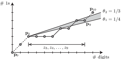
The $x$ and $y$ coordinates of $\mathbf{p}_{k}$ effectively measure the number of digits and the number of 1s respectively in the prefix string $z_{1},\ldots,z_{k}$ . See Figure 1 for an illustration.

The natural representation is useful because densities have a clear geometric interpretation:

Lemma 3.

In the natural representation, the density $D(a,b)$ is the gradient of the line segment joining $\mathbf{p}_{a-1}$ with $\mathbf{p}_{b}$ .

The proof follows directly from the definition of $D(a,b)$ . The shaded cone in Figure 1 shows how, for our example problem, the gradient of the line segment joining $\mathbf{p}_{2}$ with $\mathbf{p}_{9}$ (i.e., the density $D(3,9)$ ) lies within our target range $[\theta_{1},\theta_{2}]=[1/4,1/3]$ .

Our second geometric representation is the orthogonal representation. Intuitively, this is obtained by shearing the previous diagram so that lines of slope $\theta_{1}$ and $\theta_{2}$ become horizontal and vertical respectively, as shown in Figure 2. Formally, we define it as follows.

Definition 4.

Given a string $z_{1},\ldots,z_{n}$ and rational numbers $\theta_{1}=c_{1}/d_{1}$ and $\theta_{2}=c_{2}/d_{2}$ as described earlier, the orthogonal representation is the sequence of $n+1$ points $\mathbf{q}_{0},\ldots,\mathbf{q}_{n}$ , where each $\mathbf{q}_{k}$ has coordinates $(c_{2}k-d_{2}\sum_{i=1}^{k}z_{i},\ -c_{1}k+d_{1}\sum_{i=1}^{k}z_{i})$ .

From this definition we obtain the following immediate result.

Lemma 5.

$\mathbf{q}_{0}=(0,0)$ , and for $i>0$ we have $\mathbf{q}_{i}=\mathbf{q}_{i-1}+(c_{2},-c_{1})$ if $z_{i}=0$ or $\mathbf{q}_{i}=\mathbf{q}_{i-1}+(c_{2}-d_{2},d_{1}-c_{1})$ if $z_{i}=1$ .

The key advantage of the orthogonal representation is that densities in the target range $[\theta_{1},\theta_{2}]$ correspond to dominating points in our new coordinate system. Here we use a non-strict definition of domination: a point $(x,y)$ is said to dominate $(x^{\prime},y^{\prime})$ if and only if both $x\geq x^{\prime}$ and $y\geq y^{\prime}$ .

Theorem 6.

The density of the substring $z_{a},\ldots,z_{b}$ satisfies $\theta_{1}\leq D(a,b)\leq\theta_{2}$ if and only if $\mathbf{q}_{b}$ dominates $\mathbf{q}_{a-1}$ .

Proof.

The difference $\mathbf{q}_{b}-\mathbf{q}_{a-1}$ has coordinates

			$\displaystyle(c_{2}(b-a+1)-d_{2}\sum_{i=a}^{b}z_{i},\ -c_{1}(b-a+1)+d_{1}\sum_{i=a}^{b}z_{k})$
		$\displaystyle=$	$\displaystyle L(a,b)\cdot\left(c_{2}-d_{2}D(a,b),\ -c_{1}+d_{1}D(a,b)\right),$

which are both non-negative if and only if $D(a,b)\leq c_{2}/d_{2}=\theta_{2}$ and $D(a,b)\geq c_{1}/d_{1}=\theta_{1}$ . ∎

The shaded cone in Figure 2 shows how $\mathbf{q}_{9}$ dominates $\mathbf{q}_{2}$ in our example, indicating that the substring $z_{3},\ldots,z_{9}$ has a density in the range $[1/4,1/3]$ .

It follows that Problem 1 can be reinterpreted as:

Problem 1^′.

Given the orthogonal representation $\mathbf{q}_{0},\ldots,\mathbf{q}_{n}$ as defined above, find points $\mathbf{q}_{s},\mathbf{q}_{t}$ for which $\mathbf{q}_{t}$ dominates $\mathbf{q}_{s}$ and $t-s$ is as large as possible.

The corresponding substring that solves Problem 1 is $z_{s+1},\ldots,z_{t}$ .

We finish this section with two properties of the orthogonal representation that are key to obtaining a linear time algorithm for this problem.

Lemma 7.

The coordinates of each point $\mathbf{q}_{i}$ are integers in the range $[-n^{2},n^{2}]$ .

Proof.

This follows directly from Lemma 5: $\mathbf{q}_{0}=(0,0)$ , and the coordinates of each subsequent $\mathbf{q}_{i}$ are obtained by adding integers in the range $[-n,n]$ to the coordinates of $\mathbf{q}_{i-1}$ . ∎

Lemma 8.

If $\mathbf{q}_{i}$ dominates $\mathbf{q}_{j}$ then $i\geq j$ .

Proof.

Consider the linear function $f\colon\thinspace\mathbb{R}^{2}\to\mathbb{R}$ defined by $f(x,y)=d_{1}x+d_{2}y$ . It is clear from Lemma 5 that $f(\mathbf{q}_{0})=0$ and $f(\mathbf{q}_{i})=f(\mathbf{q}_{i-1})+d_{1}c_{2}-d_{2}c_{1}$ . Since $\theta_{1}=c_{1}/d_{1}<c_{2}/d_{2}=\theta_{2}$ it follows that $f(\mathbf{q}_{i})>f(\mathbf{q}_{i-1})$ .

Suppose $\mathbf{q}_{i}$ dominates $\mathbf{q}_{j}$ . By definition of $f$ we have $f(\mathbf{q}_{i})\geq f(\mathbf{q}_{j})$ , and by the observation above it follows that $i\geq j$ . ∎

3 Algorithm

To solve Problem ′ ‣ 2 we construct and then scan along the inner and outer frontiers, which we define as follows.

Definition 9.

Consider the orthogonal representation $\mathbf{q}_{0},\ldots,\mathbf{q}_{n}$ for the input string $z_{1},\ldots,z_{n}$ . The inner frontier is the set of points $\mathbf{q}_{k}$ that do not dominate any $\mathbf{q}_{i}$ for $i\neq k$ . The outer frontier is the set of points $\mathbf{q}_{k}$ that are not dominated by any $\mathbf{q}_{i}$ for $i\neq k$ .

Figure 3 illustrates both of these sets. They are algorithmically important because of the following result.

Lemma 10.

If $\mathbf{q}_{s}$ and $\mathbf{q}_{t}$ form a solution to Problem ′ ‣ 2, then $\mathbf{q}_{s}$ lies on the inner frontier and $\mathbf{q}_{t}$ lies on the outer frontier.

Proof.

If $\mathbf{q}_{s}$ is not on the inner frontier then $\mathbf{q}_{s}$ dominates $\mathbf{q}_{i}$ for some $i\neq s$ . By Lemma 8 we have $i<s$ , which means that $\mathbf{q}_{s}$ and $\mathbf{q}_{t}$ cannot solve Problem ′ ‣ 2 since $\mathbf{q}_{t}$ dominates $\mathbf{q}_{i}$ and $t-i>t-s$ . The argument for $\mathbf{q}_{t}$ on the outer frontier is similar. ∎

3.1 Data structures

The data structures that appear in this algorithm are simple.

For each point $\mathbf{q}_{i}=(x_{i},y_{i})$ , we refer to $i$ as the index of $\mathbf{q}_{i}$ , and we store the point as a triple $(i,x_{i},y_{i})$ . If $t$ is such a triple, we refer to its three constituents as $t.\mathit{idx}$ , $t.\mathit{x}$ and $t.\mathit{y}$ respectively.

We make frequent use of lists of triples. If $L$ is such a list, we refer to the first and last triples in $L$ as $L.\mathit{first}$ and $L.\mathit{last}$ respectively, we denote the number of triples in $L$ by $L.\mathit{size}$ , and we denote the individual triples in $L$ by $L[0]$ , $L[1]$ , …, $L[L.\mathit{size}-1]$ . All lists are assumed to have $\mathcal{O}(1)$ insertion and deletion at the beginning and end, and $\mathcal{O}(L.\mathit{size})$ iteration through the elements in order from first to last (as provided, for example, by a doubly-linked list).

For convenience we may write $\mathbf{q}_{i}\in L$ to indicate that the triple describing $\mathbf{q}_{i}$ is contained in $L$ ; formally, this means $(i,x_{i},y_{i})\in L$ .

3.2 The two-phase radix sort

The algorithm make use of a two-phase radix sort which, given a list of $\ell$ integers in the range $[0,b^{2})$ , allows us to sort these integers in $\mathcal{O}(\ell+b)$ time and space. In brief, the two-phase radix sort operates as follows.

Since the integers are in the range $[0,b^{2})$ , we can express each integer $k$ as a “two-digit number” in base $b$ ; in other words, a pair $(\alpha,\beta)$ where $k=\alpha+\beta\cdot b$ and $\alpha,\beta$ are integers in the range $0\leq\alpha,\beta<b$ .

We create an array of $b$ “buckets” (linked lists) in memory for each possible value of $\alpha$ . In a first pass, we use a counting sort to order the integers by increasing $\alpha$ (the least significant digit): this involves looping through the integers to place each integer in the bucket corresponding to the digit $\alpha$ (a total of $\ell$ distinct $\mathcal{O}(1)$ list insertion operations), and then looping through the buckets to extract the integers in order of $\alpha$ (effectively concatenating $b$ distinct lists with total length $\ell$ ). This first pass takes $\mathcal{O}(\ell+b)$ time in total.

We then make a second pass using a similar approach, using another $\mathcal{O}(\ell+b)$ counting sort to order the integers by increasing $\beta$ (the most significant digit). Importantly, the counting sort is stable and so the final result has the integers sorted by $\beta$ and then $\alpha$ ; that is, in numerical order. The total running time is again $\mathcal{O}(\ell+b)$ , and since we have $b$ buckets with a total of $\ell$ elements, the space complexity is likewise $\mathcal{O}(\ell+b)$ .

In our application, we need to sort a list of $n+1$ integers in the range $[-n^{2},n^{2}]$ ; this can be translated into the setting above with $\ell=n+1$ and $b=2n$ , and so the two-phase radix sort has $\mathcal{O}(n)$ time and space complexity.

This is a specific case of the more general radix sort; for further details the reader is referred to a standard algorithms text such as [7].

3.3 Constructing frontiers

The first stage in solving Problem ′ ‣ 2 is to construct the inner and outer frontiers in sorted order, which we do efficiently as follows. The corresponding pseudocode is given in Figure 4.

Algorithm 11.

To construct the inner frontier $I$ and the outer frontier $O$ , both in order by increasing $x$ coordinate:

1.

Build a list $L$ of triples corresponding to all $n+1$ points $\mathbf{q}_{0},\ldots,\mathbf{q}_{n}$ , using Lemma 5. Sort this list by increasing $x$ coordinate using a two-phase radix sort as described above, noting that the sort keys $x_{i}$ are all integers in the range $[-n^{2},n^{2}]$ (Lemma 7).
2.

Initialise $I$ to the one-element list $[L.\mathit{first}]$ . Step through $L$ in forward order (from left to right in the diagram); for each triple $\ell\in L$ that has lower $y$ than any triple seen before, append $\ell$ to the end of $I$ .
3.

Construct $O$ in a similar fashion, working through $L$ in reverse order (from right to left).

In step 2, there is a complication if we append a new triple $\ell$ to $I$ for which $\ell.\mathit{x}=I.\mathit{last}.\mathit{x}$ . Here we must first remove $I.\mathit{last}$ since $\ell$ makes it obsolete. See lines 12–13 of Figure 4 for the details.

1: $L\leftarrow[(0,0,0)]$ 2: for $i\leftarrow 1$ to $n$ do 3: if $z_{i}=0$ then 4: Append $L.\mathit{last}+(1,c_{2},-c_{1})$ to the end of $L$ 5: else 6: Append $L.\mathit{last}+(1,c_{2}-d_{2},d_{1}-c_{1})$ to the end of $L$ 7: Sort $L$ by increasing $x$ using a two-phase radix sort 8: 9: $I\leftarrow[L.\mathit{first}]$ 10: for all $\ell\in L$ , moving forward through $L$ do 11: if $\ell.\mathit{y}<I.\mathit{last}.\mathit{y}$ then 12: if $\ell.\mathit{x}=I.\mathit{last}.\mathit{x}$ then $\triangleright$ $I.\mathit{last}$ dominates $\ell$ 13: Remove the last triple from $I$ 14: Append $\ell$ to the end of $I$ 15: 16: $O\leftarrow[L.\mathit{last}]$ 17: for all $\ell\in L$ , moving backwards through $L$ do 18: if $\ell.\mathit{y}>O.\mathit{first}.\mathit{y}$ then 19: if $\ell.\mathit{x}=O.\mathit{first}.\mathit{x}$ then $\triangleright$ $\ell$ dominates $O.\mathit{first}$ 20: Remove the first triple from $O$ 21: Prepend $\ell$ to the beginning of $O$

Figure 4: The pseudocode for Algorithm 11

Table 1 shows a worked example for step 2 of the algorithm, i.e., the construction of the inner frontier. The points in this example correspond to Figure 3, and each row of the table shows how the frontier $I$ is updated when processing the next triple $\ell\in L$ (for simplicity we only show the coordinate pairs $(x_{i},y_{i})$ from each triple). Note that, although $L$ is sorted by increasing $x$ coordinate, for each fixed $x$ coordinate the corresponding $y$ coordinates may appear in arbitrary order.

Coordinates $(x_{i},y_{i})$	Current inner frontier $I$
from the triple $\ell\in L$
$(-10,15)$	$[\ (-10,15)\ ]$
$(-8,\phantom{0}12)$	$[\ (-10,15),\ (-8,12)\ ]$
$(-8,\phantom{0}8)$	$[\ (-10,15)\ ]$
	$[\ (-10,15),\ (-8,8)\ ]$
$(-6,\phantom{0}9)$	$[\ (-10,15),\ (-8,8)\ ]$
$(-6,\phantom{0}7)$	$[\ (-10,15),\ (-8,8)\ (-6,7)\ ]$
$(-6,\phantom{0}11)$	$[\ (-10,15),\ (-8,8)\ (-6,7)\ ]$
$(-4,\phantom{0}6)$	$[\ (-10,15),\ (-8,8)\ (-6,7)\ (-4,6)\ ]$
$(-4,\phantom{0}8)$	$[\ (-10,15),\ (-8,8)\ (-6,7)\ (-4,6)\ ]$
$(-4,\phantom{0}4)$	$[\ (-10,15),\ (-8,8)\ (-6,7)\ ]$
	$[\ (-10,15),\ (-8,8)\ (-6,7)\ (-4,4)\ ]$
$(-2,\phantom{0}5)$	$[\ (-10,15),\ (-8,8)\ (-6,7)\ (-4,4)\ ]$
$(-0,\phantom{0}0)$	$[\ (-10,15),\ (-8,8)\ (-6,7)\ (-4,4)\ (0,0)\ ]$

Table 1: Constructing the inner frontier

Theorem 12.

Algorithm 11 constructs the inner and outer frontiers in $I$ and $O$ respectively, with each list sorted by increasing $x$ coordinate, in $\mathcal{O}(n)$ time and $\mathcal{O}(n)$ space.

Proof.

This algorithm is based on a well-known method for constructing frontiers. We show here why the inner frontier $I$ is constructed correctly; a similar argument applies to the outer frontier $O$ .

If a triple $\ell\in L$ with coordinates $(x_{i},y_{i})$ does belong on the inner frontier (i.e., there is no other point $(x_{j},y_{j})$ in the list that it dominates), then we are guaranteed to add it to $I$ in step 2 because the only triples processed thus far have $x\leq x_{i}$ , and must therefore have $y>y_{i}$ . Moreover, we will not subsequently remove $\ell$ from $I$ again, since the only other triples with the same $x$ coordinate must have $y>y_{i}$ .

If a triple $\ell\in L$ with coordinates $(x_{i},y_{i})$ does not belong on the inner frontier, then there is some point $(x_{j},y_{j})$ that it dominates. If $x_{j}<x_{i}$ then we never add $\ell$ to $I$ , since by the time we process $\ell$ we will already have seen the coordinate $y_{j}$ (which is at least as low as $y_{i}$ ). Otherwise $x_{j}=x_{i}$ and $y_{j}<y_{i}$ , and so we either add and then remove $\ell$ from $I$ or else never add it at all, depending on the order in which we process the points with $x$ coordinate equal to $x_{i}$ . Either way, $\ell$ does not appear in the final list $I$ .

Therefore the list $I$ contains precisely the inner frontier; moreover, since we process the points by increasing $x$ coordinate, the list $I$ will be sorted by $x$ accordingly.

The main innovation in this algorithm is the use of a radix sort with two-digit keys, made possible by Lemma 7, which allow us to avoid the usual $\mathcal{O}(n\log n)$ cost of sorting. The two-phase radix sort runs in $\mathcal{O}(n)$ time and space, as do the subsequent list operations in Steps 2–4, and so the entire algorithm runs in $\mathcal{O}(n)$ time and space as claimed. ∎

3.4 Sliding windows

The second stage in solving Problem ′ ‣ 2 is to simultaneously scan through the inner and outer frontiers in search of possible solutions $\mathbf{q}_{s}\in I$ and $\mathbf{q}_{t}\in O$ .

We do this by trying each $\mathbf{q}_{s}$ in order on the inner frontier, and maintaining a sliding window $W$ of possible points $\mathbf{q}_{t}$ ; specifically, $W$ consists of all points on the outer frontier that dominate $\mathbf{q}_{s}$ . Figure 5 illustrates this window $W$ as $\mathbf{q}_{s}$ moves along the inner frontier from left to right.

For each point $\mathbf{q}_{s}\in I$ that we process, it is easy to update $W$ in amortised $\mathcal{O}(1)$ time using sliding window techniques (pushing new points onto the end of the list $W$ as they enter the window, and removing old points from the beginning as they exit the window). However, we still need a fast way of locating the point $\mathbf{q}_{t}\in O$ that dominates $\mathbf{q}_{s}$ and for which $t-s$ is largest. Equivalently, we need a fast way of choosing the triple $w\in W$ that maximises $w.\mathit{idx}$ .

To do this, we maintain a sub-list $M\subseteq W$ : this is a list consisting of all triples $w\in W$ that are potential maxima. Specifically, for any triple $w\in W$ , we include $w$ in $M$ if and only if there is no $w^{\prime}\in W$ for which $w^{\prime}.\mathit{x}>w.\mathit{x}$ and $w^{\prime}.\mathit{idx}>w.\mathit{idx}$ . The rationale is that, if there were such a $w^{\prime}$ , we would always choose $w^{\prime}$ over $w$ in this or any subsequent window.

As with all of our lists, we keep $M$ sorted by increasing $x$ coordinate. Note that the condition above implies that $M$ is also sorted by decreasing index. In particular, the sought-after triple $w\in W$ that maximises $w.\mathit{idx}$ is simply $M.\mathit{first}$ , which we can access in $\mathcal{O}(1)$ time.

Crucially, we can also update the sub-list $M$ in amortised $\mathcal{O}(1)$ time for each point $\mathbf{q}_{s}\in I$ that we process. As a result, this sub-list $M$ allows us to maximise $w.\mathit{idx}$ for $w\in W$ whilst avoiding a costly linear scan through the entire window $W$ .

The details are as follows; see Figure 6 for the pseudocode.

Algorithm 13.

Let the inner and outer frontiers be stored in the lists $I$ and $O$ in order by increasing $x$ coordinate, as generated by Algorithm 11. We solve Problem ′ ‣ 2 as follows.

1.

Initialise $M$ to the empty list.
2.
Step through the inner frontier $I$ in forward order. For each triple $\mathit{inner}\in I$ :
1. (a)
  
  Process new points that enter our sliding window. To do this, we scan through any new triples $\mathit{outer}\in O$ for which $\mathit{outer}.\mathit{y}\geq\mathit{inner}.\mathit{y}$ and update $M$ accordingly.
  
  Each new $\mathit{outer}\in O$ that we process has $\mathit{outer}.\mathit{x}>m.\mathit{x}$ for all $m\in M$ , so we append $\mathit{outer}$ to the end of $M$ . However, before doing this we must remove any $m\in M$ for which $m.\mathit{idx}<\mathit{outer}.\mathit{idx}$ (since such triples would violate the definition of $M$ ). Because $M$ is sorted by decreasing index, all such $m\in M$ can be found at the end of $M$ . See lines 6–10 of Figure 6.
2. (b)
  
  Remove points from $M$ that have exited our sliding window. That is, remove triples $m\in M$ for which $m.\mathit{x}<\mathit{inner}.\mathit{x}$ .
  
  Because $M$ is sorted by increasing $x$ coordinate, all such triples can be found at the beginning of $M$ . See lines 11–12 of Figure 6.
3. (c)
  
  Update the solution. The best solution to Problem ′ ‣ 2 that uses the triple $\mathit{inner}\in I$ is the pair of points $\mathbf{q}_{\mathit{inner}.\mathit{idx}},\allowbreak\mathbf{q}_{M.\mathit{first}.\mathit{idx}}$ . If the difference $M.\mathit{first}.\mathit{idx}-\mathit{inner}.\mathit{idx}$ exceeds any seen so far, record this as the new best solution.

1: $M\leftarrow[\,]$ $\triangleright$ empty list 2: $s_{\mathrm{best}}\leftarrow 0$ , $t_{\mathrm{best}}\leftarrow 0$ $\triangleright$ best solution so far 3: $\mathit{next}\leftarrow 0$ $\triangleright$ next element of $O$ to scan through 4: 5: for all $\mathit{inner}\in I$ , moving forward through $I$ do 6: while $\mathit{next}<O.\mathit{size}$ and $O[\mathit{next}].\mathit{y}\geq\mathit{inner}.\mathit{y}$ do 7: $\mathit{next}\leftarrow\mathit{next}+1$ 8: while $M.\mathit{size}>0$ and $O[\mathit{next}].\mathit{idx}>M.\mathit{last}.\mathit{idx}$ do 9: Remove the last triple from $M$ 10: Append $O[\mathit{next}]$ to the end of $M$ 11: while $M.\mathit{size}>0$ and $M.\mathit{first}.\mathit{x}<\mathit{inner}.\mathit{x}$ do 12: Remove the first triple from $M$ 13: if $M.\mathit{first}.\mathit{idx}-\mathit{inner}.\mathit{idx}>t_{\mathrm{best}}-s_{\mathrm{best}}$ then 14: $s_{\mathrm{best}}\leftarrow\mathit{inner}.\mathit{idx}$ 15: $t_{\mathrm{best}}\leftarrow M.\mathit{first}.\mathit{idx}$

Figure 6: The pseudocode for Algorithm 13

Theorem 14.

Algorithms 11 and 13 together solve Problem ′ ‣ 2 in $\mathcal{O}(n)$ time and $\mathcal{O}(n)$ space.

Proof.

Theorem 12 analyses Algorithm 11, and the preceding discussion shows the correctness of Algorithm 13. All that remains is to verify that Algorithm 13 runs in $\mathcal{O}(n)$ time and space.

Each triple $t\in O$ is added to $M$ at most once and removed from $M$ at most once, and so the while loops on lines 6, 8 and 11 each require total $\mathcal{O}(n)$ time as measured across the entire algorithm. Finally, the outermost for loop (line 4) iterates at most $n+1$ times, giving an overall running time for Algorithm 13 of $\mathcal{O}(n)$ .

Each of the lists $I$ , $O$ and $M$ contains at most $n+1$ elements, and so the space complexity is $\mathcal{O}(n)$ also. ∎

4 Performance

Here we experimentally compare our new algorithm against the prior state of the art, namely the $\mathcal{O}(n\log n)$ algorithm of Hsieh et al. [14]. Our trials involve searching for GC-rich regions in the human genome assembly GRCh37.p2 from GenBank [2, 16]. The implementation that we use for our new algorithm is available online,¹¹ 1 For C++ implementations of all algorithms in this paper, visit http://www.maths.uq.edu.au/ $\sim$ bab/code/. and the code for the prior $\mathcal{O}(n\log n)$ algorithm was downloaded from the respective authors’ website.²² 2 The implementation of the prior algorithm [14] is taken from http://venus.cs.nthu.edu.tw/~eric/FIF.htm. Both implementations are written in C/C++.

Figure 7 measures running times for $24\times 4\times 3=288$ instances of Problem 1: we begin with 24 human chromosomes (1–22, X and Y), extract initial strings of four different lengths $n$ (ranging from $n=100\,000$ to $n=3\,000\,000$ ), and search each for the longest substring whose GC-density is constrained according to one of three different ranges $[\theta_{1},\theta_{2}]$ .

These ranges are: $[0.6326,\,0.7428]$ , which matches the first CpG island class of Ioshikhes and Zhang [17]; $[0.69905,\,0.69915]$ , which surrounds the median of this class and measures performance for a narrow density range; and $[2/3,\,3/4]$ , which measures performance when the key parameters $d_{1}$ and $d_{2}$ are very small.

The results are extremely pleasing: in every case the new algorithm runs at least $10\times$ faster than the prior state of the art, and in some cases up to $42\times$ faster. Of course such comparisons cannot be exact or fair, since the two implementations are written by different authors; however, they do illustrate that the new algorithm is not just asymptotically faster in theory (as proven in Theorem 14), but also fast in practice (i.e., the constants are not so large as to eliminate the theoretical benefits for reasonable inputs).

The results for the range $[2/3,\,3/4]$ highlight how our algorithm benefits from small denominators (in which the range of possible $x$ and $y$ coordinates becomes much smaller).

Memory becomes a significant problem when dealing with very large data sets. The algorithm of Hsieh et al. [14] uses “heavy” data structures with large memory requirements: for $n=3\,000\,000$ it uses $1.64$ GB of memory. In contrast, our new algorithm has a much smaller footprint—just $70$ MB for the same $n$ —and can thereby process values of $n$ that are orders of magnitude larger. In Figure 8 we run our algorithm over the full length of each chromosome; even the worst case (chromosome 1) with $n=249\,250\,621$ runs for all density ranges in under 85 seconds, using $5.6$ GB of memory.

All trials were run on a single 3 GHz Intel Core i7 CPU. Input and output are included in running times, though detailed measurements show this to be insignificant for both algorithms (which share the same input and output routines).

5 Related Problems

The techniques described in this paper extend beyond Problem 1. Here we examine two related problems from the bioinformatics literature, and for each we outline new algorithms that improve upon the prior state of the art. As usual, all problems take an input string $z_{1},\ldots,z_{n}$ where each $z_{i}$ is 0 or 1.

The new algorithms in this section rely on van Emde Boas trees [22], a tree-based data structure for which many elementary key-based operations have $\mathcal{O}(n\log\log n)$ time complexity. We briefly review this data structure before presenting the two related problems and the new algorithms to solve them.

5.1 van Emde Boas trees

Here we briefly recall the essential ideas behind van Emde Boas trees. For full details we refer the author to a modern textbook on algorithms such as [7].

A van Emde Boas tree is a data structure that implements an associative array (mapping keys to values), in which the user can perform several elementary operations in $\mathcal{O}(\log m)$ time, where $m$ is the number of bits in the key. These elementary operations include inserting or deleting a key-value pair, looking up the value stored for a given key, and looking up the successor or predecessor of a given key $k$ (i.e., the first key higher or lower than $k$ respectively). In our case, all keys are in the range $[-n^{2},n^{2}]$ (Lemma 7), and so $m\in\mathcal{O}(\log n^{2})=\mathcal{O}(\log n)$ ; that is, these elementary operations run in $\mathcal{O}(\log\log n)$ time.

The core idea of this data structure is that each node of the tree represents a range of $p$ consecutive possible keys for some $p$ , and has $\sqrt{p}$ children (each a smaller van Emde Boas tree) that each represent a sub-range of $\sqrt{p}$ possible keys. Each node also maintains the minimum and maximum keys that are actually present within its range. The root node of the tree represents the complete range of $2^{m}$ possible keys.

Furthermore, for each node $V$ of the tree representing a range of $p$ possible keys, we also maintain an auxiliary van Emde Boas tree that stores which of the $\sqrt{p}$ children of $V$ are non-empty (i.e., have at least one key stored within them).

To look up the successor of a given key $k$ we travel down the tree, and each time we reach some node $V_{i}$ that represents $p_{i}$ potential keys, we identify which of the $\sqrt{p_{i}}$ children contains the successor of $k$ by examining the auxiliary tree attached to $V_{i}$ . This induces a query on the auxiliary tree (representing $\sqrt{p_{i}}$ potential non-empty child trees) followed by a query on the selected child (representing $\sqrt{p_{i}}$ potential keys), and so the running time follows a recurrence of the form $T(m)=2T(m/2)+O(1)$ ; solving this recurrence yields the overall $\mathcal{O}(log(m))$ time complexity. The running times for inserting and deleting keys follow a similar argument, and again we refer the reader to a text such as [7] for the details.

5.2 Shortest substring in a density range

The first related problem that we consider is a natural counterpart to Problem 1: instead of searching for the longest substring under given density constraints, we search for the shortest.

Problem 15.

Find the shortest substring whose density lies in a given range. That is, given rationals $\theta_{1}<\theta_{2}$ , compute

\min_{1\leq a\leq b\leq n}\left\{L(a,b)\,|\,\theta_{1}\leq D(a,b)\leq\theta_{2}\right\}.

The best known algorithm for this problem runs in $\mathcal{O}(n\log n)$ time [14]; here we improve this to $\mathcal{O}(n\log\log n)$ .

By Theorem 6 and Lemma 8, this is equivalent to finding points $\mathbf{q}_{s}\neq\mathbf{q}_{t}$ for which $\mathbf{q}_{t}$ dominates $\mathbf{q}_{s}$ and for which $t-s$ is as small as possible. To do this, we iterate through each possible endpoint $\mathbf{q}_{t}$ in turn, and maintain a partial outer frontier $P$ consisting of all non-dominated points amongst the previous points $\{\mathbf{q}_{0},\mathbf{q}_{1},\ldots,\mathbf{q}_{t-1}\}$ ; that is, all points $\mathbf{q}_{i}$ ( $0\leq i\leq t-1$ ) that are not dominated by some other $\mathbf{q}_{j}$ ( $i<j\leq t-1$ ). When examining a candidate endpoint $\mathbf{q}_{t}$ , it is straightforward to show that any optimal solution $\mathbf{q}_{s},\mathbf{q}_{t}$ must satisfy $\mathbf{q}_{s}\in P$ .

Algorithm 16.

To solve Problem 15:

1.

Initialise $P$ to the empty list.
2.
For each $t=0,\ldots,n$ in turn, try $\mathbf{q}_{t}$ as a possible endpoint:
1. (a)
  
  Update the solution. To do this, walk through all points $\mathbf{q}_{s}\in P$ that are dominated by $\mathbf{q}_{t}$ . If the difference $t-s$ is smaller than any seen so far, record this as the new best solution.
2. (b)
  
  Update the partial frontier. To do this, remove all $\mathbf{q}_{s}\in P$ that are dominated by $\mathbf{q}_{t}$ , and then insert $\mathbf{q}_{t}$ into $P$ .

The key to a fast time complexity is choosing an efficient data structure for storing the partial outer frontier $P$ . We keep $P$ sorted by increasing $x$ coordinate, and for the underlying data structure we use a van Emde Boas tree [22].

To walk through all points $\mathbf{q}_{s}\in P$ that are dominated by $\mathbf{q}_{t}$ in step 2a, we locate the point $\mathbf{p}\in P$ with smallest $x$ coordinate larger than $x_{t}$ ; a van Emde Boas tree can do this in $\mathcal{O}(\log\log n)$ time. The dominated points $\mathbf{q}_{s}$ can then be found immediately prior to $\mathbf{p}$ in the partial frontier. Adding and removing points in step 2b is likewise $\mathcal{O}(\log\log n)$ time, and the overall space complexity of a van Emde Boas tree can be made $\mathcal{O}(n)$ [7].

A core requirement of this data structure is that keys in the tree can be described by integers in the range $0,\ldots,n$ . To arrange this, we pre-sort the $x$ coordinates $\mathbf{q}_{0}.\mathit{x},\ldots,\mathbf{q}_{n}.\mathit{x}$ using an $\mathcal{O}(n)$ two-phase radix sort (as described in Section 3.2) and then replace each $x$ coordinate with its corresponding rank.

To finalise the time and space complexities, we observe that each point $\mathbf{q}_{s}\in P$ that is processed in step 2a is immediately removed in step 2b, and so no point is processed more than once. Combined with the preceding discussion, this gives:

Theorem 17.

Algorithm 16 runs in $\mathcal{O}(n\log\log n)$ time and uses $\mathcal{O}(n)$ space.

We can add an optional length constraint to Problem 15: given rationals $\theta_{1}<\theta_{2}$ and length bounds $L_{1}<L_{2}$ , find the shortest substring $z_{a},\ldots,z_{b}$ for which $\theta_{1}\leq D(a,b)\leq\theta_{2}$ and $L_{1}\leq L(a,b)\leq L_{2}$ . This is a simple modification to Algorithm 16: we redefine the partial frontier $P$ to be the set of all non-dominated points amongst $\{\mathbf{q}_{0},\mathbf{q}_{1},\ldots,\mathbf{q}_{t-L_{1}}\}$ . The update procedure changes slightly, but the $\mathcal{O}(n\log\log n)$ running time remains.

5.3 Maximal collection of substrings in a density range

The second related problem involves searching for substrings “in bulk”: instead of finding the longest substring under given density constraints, we find the most disjoint substrings.

Problem 18.

Find a maximum cardinality set of disjoint substrings whose densities all lie in a given range. That is, given rationals $\theta_{1}<\theta_{2}$ , find substrings $(z_{a_{1}},\ldots,z_{b_{1}})$ , $(z_{a_{2}},\ldots,z_{b_{2}})$ , …, $(z_{a_{k}},\ldots,z_{b_{k}})$ where $\theta_{1}\leq D(a_{i},b_{i})\leq\theta_{2}$ and $b_{i}<a_{i+1}$ for each $i$ , and where $k$ is as large as possible.

As before, the best known algorithm runs in $\mathcal{O}(n\log n)$ time [14]; again we improve this bound to $\mathcal{O}(n\log\log n)$ .

For this problem we mirror the greedy approach of Hsieh et al. [14]. One can show that, if $z_{a},\ldots,z_{b}$ is a substring of density $\theta_{1}\leq D(a,b)\leq\theta_{2}$ with minimum endpoint $b$ , then some optimal solution to Problem 18 has $b_{1}=b$ (i.e., we can choose $z_{a},\ldots,z_{b}$ as our first substring). See [14, Lemma 6].

Our strategy is to use our previous Algorithm 16 to locate such a substring $z_{a},\ldots,z_{b}$ , store this as part of our solution, and then rerun our algorithm on the leftover $n-b$ input digits $z_{b+1},\ldots,z_{n}$ . We repeat this process until no suitable substring can be found.

Algorithm 19.

To solve Problem 18:

1.

Initialise $i\leftarrow 1$ .
2.

Run Algorithm 16 on the input string $z_{i},\ldots,z_{n}$ , but terminate Algorithm 16 as soon as any dominating pair $\mathbf{q}_{s},\mathbf{q}_{t}$ is found.
3.

If such a pair is found: add the corresponding substring $z_{s+1},\ldots,z_{t}$ to our solution set, set $i\leftarrow t+1$ , and return to step 2. Otherwise terminate this algorithm.

It is important to reuse the same van Emde Boas tree on each run through Algorithm 16 (simply empty out the tree each time), so that the total initialisation cost remains $\mathcal{O}(n\log\log n)$ .

Theorem 20.

Algorithm 19 runs in $\mathcal{O}(n\log\log n)$ time and requires $\mathcal{O}(n)$ space.

Proof.

Running Algorithm 16 in step 2 takes $\mathcal{O}([t-i]\allowbreak\log\log n)$ time, since it only examines points $\mathbf{q}_{i},\ldots,\mathbf{q}_{t}$ before the dominating pair is found. The total running time of Algorithm 19 is therefore $\mathcal{O}(b_{1}\log\log n+[b_{2}-b_{1}]\log\log n+\ldots+[b_{k}-b_{k-1}]\log\log n)=\mathcal{O}(n\log\log n)$ . The $\mathcal{O}(n)$ space complexity follows from Theorem 17 plus the observation that the final solution set can contain at most $n$ disjoint substrings. ∎

As before, it is simple to add a length constraint to Problem 18, so that each substring $z_{a_{i}},\ldots,z_{b_{i}}$ must satisfy both $\theta_{1}\leq D(a_{i},b_{i})\leq\theta_{2}$ and $L_{1}\leq L(a_{i},b_{i})\leq L_{2}$ for some length bounds $L_{1}<L_{2}$ . We simply incorporate the length constraint into Algorithm 16 as described in Section 5.2, and nothing else needs to change.

5.4 Performance

As before, we have implemented both Algorithms 16 and 19 and tested each against the prior state of the art using human genomic data, following the same procedures as described in Section 4. Our van Emde Boas tree implementation is based on the MIT-licensed libveb by Jani Lahtinen, available from http://code.google.com/p/libveb/.

For the shortest substring problem, our algorithm runs at 12–62 times the speed of the prior algorithm [14], and requires under $1/50$ th of the memory. For finding a maximal collection of substrings, our algorithm runs at 0.94–13 times the speed of the prior algorithm [14], and uses less than $1/20$ th of the memory.³³ 3 The few cases in which our algorithm was slightly slower (down to $0.94$ times the speed) all involved large denominators $d_{1},d_{2}$ and maximal collections involving a very large number of very short substrings.

Once again, these improvements—particularly for memory usage—allow us to run our algorithms with significantly larger values of $n$ than for the prior state of the art. For chromosome 1 with $n=249\,250\,621$ , the two algorithms run in 221 and 176 seconds respectively, both using approximately 5.6 GB of memory.

6 Discussion

In this paper we consider three problems involving the identification of regions in a sequence where some feature occurs within a given density range. For all three problems we develop new algorithms that offer significant performance improvements over the prior state of the art. Such improvements are critical for disciplines such as bioinformatics that work with extremely large data sets.

The key to these new algorithms is the ability to exploit discreteness in the input data. All of the applications we consider (GC-rich regions, CpG islands and sequence alignment) can be framed in terms of sequences of 1s and 0s. Such discrete representations are powerful: through Lemma 7, they allow us to perform $\mathcal{O}(n)$ two-phase radix sorts, and to reindex coordinates by rank for van Emde Boas trees. In this way, discreteness allows us to circumvent the theoretical $\Omega(n\log n)$ bounds of Hsieh et al. [14], which are only proven for the more general continuous (non-discrete) setting.

In a discrete setting, an obvious lower bound for all three problems is $\Omega(n)$ time (which is required to read the input sequence). For the first problem (longest substring with density in a given range), we attain this best possible lower bound with our $\mathcal{O}(n)$ algorithm. This partially answers a question of Chen and Chao [6], who ask in a more general setting whether such an algorithm is possible.

For the second and third problems (shortest substring and maximal collection of substrings), although our $\mathcal{O}(n\log\log n)$ algorithms have smaller time complexity and better practical performance than the prior state of the art, there is still room for improvement before we reach the theoretical $\Omega(n)$ lower bound (which may or may not be possible). Further research into these questions may prove fruitful.

The techniques we develop here have applications beyond those discussed in this paper. For example, consider the problem of finding the longest substring whose density matches a precise value $\theta$ . This close relative of Problem 1 has cryptographic applications [4]. An $\mathcal{O}(n)$ algorithm is known [5], but it requires a complex linked data structure. By adapting and simplifying Algorithms 11 and 13 for the case $\theta_{1}=\theta_{2}=\theta$ , we obtain a new $\mathcal{O}(n)$ algorithm with comparable performance and a much simpler implementation.

This last point raises the question of whether our algorithms for the second and third problems can likewise be simplified to use only simple array-based sorts and scans instead of the more complex van Emde Boas trees. Further research in this direction may yield new practical improvements for these algorithms.

Acknowledgements

This work was supported by the Australian Research Council (grant number DP1094516).

References

[1] Lloyd Allison, Longest biased interval and longest non-negative sum interval, Bioinformatics 19 (2003), no. 10, 1294–1295.
[2] Dennis A. Benson, Ilene Karsch-Mizrachi, David J. Lipman, James Ostell, and David L. Wheeler, GenBank, Nucleic Acids Res. 36 (2008), no. suppl 1, D25–D30.
[3] Giorgio Bernardi, Isochores and the evolutionary genomics of vertebrates, Gene 241 (2000), no. 1, 3–17.
[4] Serdar Boztaş, Simon J. Puglisi, and Andrew Turpin, Testing stream ciphers by finding the longest substring of a given density, Information Security and Privacy, Lecture Notes in Comput. Sci., vol. 5594, Springer, Berlin, 2009, pp. 122–133.
[5] Benjamin A. Burton, Searching a bitstream in linear time for the longest substring of any given density, Algorithmica 61 (2011), no. 3, 555–579.
[6] Kuan-Yu Chen and Kun-Mao Chao, Optimal algorithms for locating the longest and shortest segments satisfying a sum or an average constraint, Inform. Process. Lett. 96 (2005), no. 6, 197–201.
[7] Thomas H. Cormen, Charles E. Leiserson, Ronald L. Rivest, and Clifford Stein, Introduction to algorithms, 3rd ed., MIT Press, Cambridge, MA, 2009.
[8] Laurent Duret, Dominique Mouchiroud, and Christian Gautier, Statistical analysis of vertebrate sequences reveals that long genes are scarce in GC-rich isochores, J. Mol. Evol. 40 (1995), no. 3, 308–317.
[9] Manel Esteller, CpG island hypermethylation and tumor suppressor genes: A booming present, a brighter future, Oncogene 21 (2002), no. 35, 5427–5440.
[10] Stephanie M. Fullerton, Antonio Bernardo Carvalho, and Andrew G. Clark, Local rates of recombination are positively correlated with GC content in the human genome, Mol. Biol. Evol. 18 (2001), no. 6, 1139–1142.
[11] Michael H. Goldwasser, Ming-Yang Kao, and Hsueh-I Lu, Linear-time algorithms for computing maximum-density sequence segments with bioinformatics applications, J. Comput. System Sci. 70 (2005), no. 2, 128–144.
[12] Ronald I. Greenberg, Fast and space-efficient location of heavy or dense segments in run-length encoded sequences, Computing and Combinatorics, Lecture Notes in Comput. Sci., vol. 2697, Springer, Berlin, 2003, pp. 528–536.
[13] Ross Hardison, Dan Krane, David Vandenbergh, Jan-Fang Cheng, James Mansberger, John Taddie, Scott Schwartz, Xiaoqiu Huang, and Webb Miller, Sequence and comparative analysis of the rabbit $\alpha$ -like globin gene cluster reveals a rapid mode of evolution in a $\mbox{G}+\mbox{C}$ -rich region of mammalian genomes, J. Mol. Biol. 222 (1991), no. 2, 233–249.
[14] Yong-Hsiang Hsieh, Chih-Chiang Yu, and Biing-Feng Wang, Optimal algorithms for the interval location problem with range constraints on length and average, IEEE/ACM Trans. Comput. Biol. Bioinformatics 5 (2008), no. 2, 281–290.
[15] Xiaoqiu Huang, An algorithm for identifying regions of a DNA sequence that satisfy a content requirement, Comput. Appl. Biosci. 10 (1994), no. 3, 219–225.
[16] International Human Genome Sequencing Consortium, Finishing the euchromatic sequence of the human genome, Nature 431 (2004), no. 7011, 931–945.
[17] Ilya P. Ioshikhes and Michael Q. Zhang, Large-scale human promoter mapping using CpG islands, Nat. Genetics 26 (2000), no. 1, 61–63.
[18] Frank Larsen, Glenn Gundersen, Rodrigo Lopez, and Hans Prydz, CpG islands as gene markers in the human genome, Genomics 13 (1992), no. 4, 1095–1107.
[19] Yaw-Ling Lin, Tao Jiang, and Kun-Mao Chao, Efficient algorithms for locating the length-constrained heaviest segments, with applications to biomolecular sequence analysis, Mathematical Foundations of Computer Science 2002, Lecture Notes in Comput. Sci., vol. 2420, Springer, Berlin, 2002, pp. 459–470.
[20] Serge Saxonov, Paul Berg, and Douglas L. Brutlag, A genome-wide analysis of CpG dinucleotides in the human genome distinguishes two distinct classes of promoters, Proc. Natl. Acad. Sci. USA 103 (2006), no. 5, 1412–1417.
[21] Paul M. Sharp, Michalis Averof, Andrew T. Lloyd, Giorgio Matassi, and John F. Peden, DNA sequence evolution: The sounds of silence, Phil. Trans. R. Soc. Lond. B 349 (1995), no. 1329, 241–247.
[22] P. van Emde Boas, R. Kaas, and E. Zijlstra, Design and implementation of an efficient priority queue, Math. Systems Theory 10 (1977), no. 1, 99–127.
[23] Lusheng Wang and Ying Xu, SEGID: Identifying interesting segments in (multiple) sequence alignments, Bioinformatics 19 (2003), no. 2, 297–298.
[24] Serguei Zoubak, Oliver Clay, and Giorgio Bernardi, The gene distribution of the human genome, Gene 174 (1996), no. 1, 95–102.

Benjamin A. Burton
School of Mathematics and Physics, The University of Queensland
Brisbane QLD 4072, Australia
(bab@maths.uq.edu.au)

Mathias Hiron
Izibi, 7, rue de Vaugrenier
89190 St Maurice R.H, France
(mathias.hiron@gmail.com)

Locating regions in a sequence under density constraints

Abstract

1 Introduction

2 Mathematical Framework

Problem 1.

Definition 2.

Lemma 3.

Definition 4.

Lemma 5.

Theorem 6.

Proof.

Problem 1′.

Lemma 7.

Proof.

Lemma 8.

Proof.

3 Algorithm

Definition 9.

Lemma 10.

Proof.

3.1 Data structures

3.2 The two-phase radix sort

3.3 Constructing frontiers

Algorithm 11.

Theorem 12.

Proof.

3.4 Sliding windows

Algorithm 13.

Theorem 14.

Proof.

4 Performance

5 Related Problems

5.1 van Emde Boas trees

5.2 Shortest substring in a density range

Problem 15.

Algorithm 16.

Theorem 17.

5.3 Maximal collection of substrings in a density range

Problem 18.

Algorithm 19.

Theorem 20.

Proof.

5.4 Performance

6 Discussion

Acknowledgements

References

Problem 1^′.