Adaptive Single–Trial Error/Erasure Decoding of Reed–Solomon CodesThanks: Parts of this work have been presented at the recent results poster session of IEEE ISIT 2010. The authors have been supported by DFG, Germany, under grants BO 867/22-1 and BO 867/21-1. Vladimir Sidorenko is on leave from IITP, Russian Academy of Sciences, Moscow, Russia.
Abstract
Algebraic decoding algorithms are commonly applied for the decoding of Reed–Solomon codes. Their main advantages are low computational complexity and predictable decoding capabilities. Many algorithms can be extended for correction of both errors and erasures. This enables the decoder to exploit binary quantized reliability information obtained from the transmission channel: Received symbols with high reliability are forwarded to the decoding algorithm while symbols with low reliability are erased. In this paper we investigate adaptive single–trial error/erasure decoding of Reed–Solomon codes, i.e. we derive an adaptive erasing strategy which minimizes the residual codeword error probability after decoding. Our result is applicable to any error/erasure decoding algorithm as long as its decoding capabilities can be expressed by a decoder capability function. Examples are Bounded Minimum Distance decoding with the Berlekamp–Massey- or the Sugiyama algorithms and the Guruswami–Sudan list decoder.
I Introduction
Using algebraic error/erasure decoders for pseudo–soft decoding of Reed–Solomon (RS) codes dates back to Forney [1, 2]. His Generalized Minimum Distance (GMD) decoding applies an error/erasure decoder multiple times, each time with an increased number of erased most unreliable symbols of the received word. In very good channels, the residual codeword error probability of GMD decoding approaches that of Maximum Likelihood (ML) decoding if the number of such decoding trials is sufficiently large, i.e. , where is the minimum Hamming distance of the RS code. Thus, the computational complexity of GMD decoding is –times that of errors–only decoding. Roughly, we can say , which means that quadratic decoding complexity in the code length becomes cubic and so on. Kötter [3] provided a modification of the Berlekamp–Massey algorithm that essentially computes all decoding trials at once, i.e. without increasing complexity. A similar result was achieved in [4, 5] for the Euclidean algorithm and in [6] using Newton interpolation. Up to our knowledge, there is no such modification of Guruswami–Sudan (GS) [7] list decoding – which can be considered as state of the art in algebraic decoding – so far. However, Kötter and Vardy provided a modification of the GS algorithm that is capable of exploiting soft information [8].
GMD decoding is per se a fixed approach, i.e. the erasing strategy is constant for each received word. Adaptive variants have been investigated in [9, 10, 11]. The respective authors show that the number of decoding trials can be reduced significantly, if the erasing strategy is optimally calculated for every single received word. The aforementioned papers focus on the maximization of the achievable decoding radius, i.e. the maximum correctable number of errors in the received word. In contrast to that, our objective is to minimize the residual codeword error probability after decoding. We achieve this using a technique first introduced in 2010 [12] for optimal error/erasure decoding of binary codes. As in the latter paper, we restrict ourselves to one single decoding trial, i.e. , for simplicity.
The rest of the paper is organized as follows. In Section II we give an overview of error/erasure decoding and introduce the required notations. We introduce the decoder capability function which allows to derive the optimal erasing strategy in a general manner. Here and in the following, optimal means minimizing the residual codeword error probability. In Section III, we derive an optimal adaptive erasing strategy for one single decoding trial. Section IV describes two computationally efficient approximations of the optimal strategy, one of them with complexity quadratic in the code length . In Section V we show the potential of single–trial error/erasure decoding in terms of achievable residual codeword error probability as well as the quality of the two approximative variants by simulation. The paper is wrapped up with conclusions and an outlook in Section VI.
II Reliability–Based Error/Erasure Decoding and Decoder Capability Functions
Consider the RS code of length , dimension and minimum distance over the extension field . Thereby, for some prime number and some integer . The transmitter encodes an information vector into a codeword . Each symbol , , is mapped to a symbol of a modulation alphabet resulting in the modulated codeword . This modulated codeword is transmitted over the channel, where it is distorted by two–dimensional Additive White Gaussian Noise (AWGN). At the receiver, the received word is obtained. It is the sum of the modulated codeword and an error word . Each symbol is mapped to the closest (in Euclidean metric) modulation point of , the result of this procedure is the hard decision of . This hard decision can be fed into the inverse mapper function to obtain a received vector , which in turn can be fed into any algebraic hard decision decoder for .
The hard decision, i.e. the mapping from received symbols to closest modulation points , is error–prone since it is not necessarily correct: The received might be closest in Euclidean metric to an . We refer to the probability of an incorrect hard decision as unreliability of a received symbol and denote it by . Here,
is the AWGN standard deviation for given in dB. Note that due to the one–to–one mapping between and we can as well write the unreliability as a function of the de–modulated received symbols, i.e. . By definition, we have
| (1) |
where the last equality follows from the assumption of equiprobable codeword symbols. In practice, the calculation of (1) is not feasible for large modulation alphabets , hence we use the nearest neighbor approximation
| (2) |
where is the set of nearest neighbors of . This allows to store all possible values of in a comparatively small lookup table as the following example demonstrates.
Assume –Quadrature Amplitude Modulation (QAM) with average signal energy one, Gray mapping and –bit–quantization. Without nearest neighbor approximation, this leads to a lookup table with entries, each containing two integers for the coordinates and one real number for the unreliability value . Considering only the nearest neighbors, the lookup table consists of only such entries if symmetries within the QAM decision regions are exploited. This allows to store lookup tables for many different values, e.g. up to the precision of the (required) channel estimation. Fig. 1 shows a density plot of for the complete Euclidean plane, the black dots mark the modulation points, darker color marks higher unreliability. Note that the unreliabilities for most decision regions are either rotated versions of each other or they coincide. Furthermore, the unreliabilities of the decision regions are either point symmetric to their modulation point (regions in the center) or symmetric to a line through the modulation point (border and corner regions). This allows to discard of the quantization intervals in the first case and of the intervals in the second case.

At the receiver, the unreliability is calculated (or taken from the lookup table) for every received symbol , . W.l.o.g. we assume here and in the following that the received word is ordered according to its symbol’s unreliabilities, i.e. . The idea of error/erasure decoding is to discard the most unreliable symbols (i.e. to erase them) since it is likely that they are erroneous. Instead of , the input vector fed into the algebraic decoder is then
where the first symbols are replaced by the erasure marker . In order to do this, two conditions need to be fulfilled. First, we require an algebraic decoder which is capable of decoding both errors and erasures. Second, we must be capable of deciding how many of the most unreliable symbols should be discarded.
Algebraic error/erasure decoders for RS codes are well–known. Classical Bounded Minimum Distance (BMD) e.g. decoding using the Berlekamp–Massey- or the Sugiyama algorithms can be augmented by an erasure option [13] as can the GS list decoder [7]. In [14], a decoder with erasure option for Interleaved Reed–Solomon (IRS) codes from [15] is applied to decode –punctured RS codes.
The decoder capability function (DCF) of an algebraic error/erasure decoder is an inequality of the form
which is true whenever the decoder can correct errors and erasures in any given received word. Three important examples for error/erasure decoders and their respective are given in Table I.
| Decoder | ||
|---|---|---|
| Bounded Minimum Distance | ||
| IRS–based (for –punctured RS codes) | ||
| Guruswami–Sudan, |
Based on the DCF of a decoder, it is straightforward to calculate the maximal number of correctable errors for any given number of erasures in a received word, i.e. the maximal number which fulfills the DCF for fixed . We denote this number of errors by , where , , is the number of erasures. Table I shows for the three considered decoders.
III Optimal Erasing Strategy
In this section, we shall solve the following basic problem of adaptive single–trial error/erasure decoding. Thereby, our technique is similar to [12].
Problem 1
For given received vector with ordered unreliability values and channel state , find the optimal number , , of erased most unreliable symbols, such that the residual codeword error probability of decoding using a decoder with DCF is minimized.
The foundation of our solution is basic probability theory and our aim is to express the residual codeword error probability as a function of the number of erased most unreliable symbols. In the following, we omit all subindices for simpler reading. However, the reader should keep in mind that all functions and values depend on .
Given a received vector , we define the binary random variables , , by
By definition of , the probabilities of the two possible outcomes of are and . Thus, the probability generating function (PGF) of is
After erasing symbols from , there are , , erroneous symbols within the non–erased symbols of . We denote their number by the discrete random variable
with PGF
Using the PGF of , the probability for errors in the non–erased symbols can be calculated by
where the superscript (ε) denotes the -th derivative.
Decoding is successful if and fails otherwise. Hence, we can state the residual codeword error probability after decoding by
| (3) |
Consequently, the optimal choice of (solving Problem 1) is
| (4) |
IV Computationally Efficient Erasing Strategies
In this section, we give two approximations of which eventually allow to calculate approximative with complexities in and , respectively.
IV-A Approximation based on the Hoeffding Bound
Given a set of independent random variables fulfilling certain properties, the Hoeffding bound [16] states that the probability of this sum to assume values outside a small discrete interval around its expectation is exponentially small. We show in [12] that the , , and their partial sum have these properties, leading to the inequality
where is a parameter that denotes the one–directional size of
Setting guarantees that the share of the probabilities for in the calculation (3) of is small, cf. Table II.
| Partial Sum | Share in |
|---|---|
As a result, all values in (3) can be neglected and a good approximation of the residual codeword error probability is obtained by
In [12], the complexity of adaptive single–trial error/erasure decoding of binary codes with the Hoeffding approximation of is stated to be in , this also holds for our case of (non–binary) RS codes.
IV-B Approximation based on
For the second approximation, we require the following proposition. So far it is verified only by experiments and we are working on a proof.
Proposition 1
For fixed , , is a unimodal function in and its mode is determined by the expectation .
Fig. 2 shows a D plot of for all , , each slice in –direction is unimodal according to Proposition 1 and each coincides with the mode of the respective .
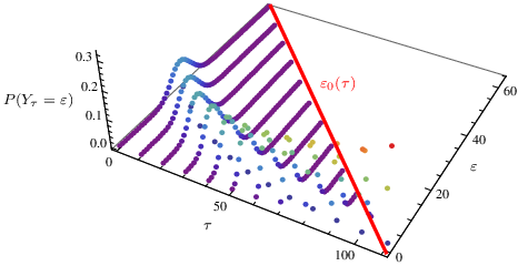
If the expectation is smaller than the error boundary, i.e. if , then we can approximate the sum by its largest element, which is . Analogously, if , then is a good approximation of the sum . Inserting into (3) gives
Based on the complexity analysis of the Hoeffding approximation in [12], it is easy to see that the complexity of the approximation is in . Since there are no practical decoders with lower complexity than , adaptive single–trial error/erasure decoding is in the same complexity class as the error/erasure decoder itself and the computation of increases complexity only by an additive constant.
V Simulation Results
We investigate the potential of adaptive single–trial error/erasure decoding for the RS code . Two error/erasure decoders are considered: The classical BMD decoder (e.g. Berlekamp–Massey or Sugiyama) and the GS list decoder with multiplicities .
Performance evaluation is done by simulation and by semi–simulative upper bounds of the residual codeword error probability. For each considered , we calculate an average unreliability vector , , by averaging over random unreliability vectors. For each variant of (exact, Hoeffding approximation, approximation), we calculate for according to (4). We use for every received vector, which means that the simulation is in fact non-adaptive, using the optimal erasing strategy for the average unreliability vector. The resulting residual codeword error probability curves are indeed upper bounds, it is clear that the error probability can not be higher when is calculated for every single received vector. Precise error probabilities of errors–only decoding are obtained by inserting into (3).

The approximation is considered in Fig. 3. It shows actual simulation results for dB and the aforementioned upper bound for dB. Clearly, adaptive single–trial error/erasure decoding with a classical BMD decoder yields a gain of approximately dB for practical error probabilities. For the GS list decoder, the achievable gain is negligible. The reason for this lies in the non–linearity of the GS list decoder’s function, whose slope gets steeper with decreasing . This means that the benefit of transforming errors into erasures diminishes for a small number of erased symbols. The residual codeword probability curve of Forney’s original –trial GMD decoding [1, 2] is given as a reference. Fig. 3 shows that most of GMD’s gain can be achieved by a single adaptive trial, if only the erasing strategy is chosen optimally.
Fig. 4 shows for an interesting range of residual codeword error probabilities that there is virtually no difference between exact calculation of and the two proposed approximations. Our recommendation is to use the approximation whenever exact calculation of is prohibitive. It is feasible both in terms of computational complexity () and approximation quality.

VI Conclusions
Classical error/erasure BMD decoders for RS codes are widely deployed. We presented an adaptive single–trial error/erasure decoding technique, which allows to decrease the residual codeword error probability of such decoders using a low–complexity, i.e. , pre–computation step. The achievable gain of our technique is around dB for . This is slightly less than the gain of GMD decoding but neither does it require a modification of the decoder itself (Kötter’s fast GMD decoder [3]) nor does it require decoding trials (Forney’s original GMD decoder [1, 2]). Our technique is general, it can be applied to any error/erasure decoder as long as its DCF is known.
Acknowledgments
The authors would like to thank Dejan E. Lazich for carefully proofreading the manuscript.
References
- [1] G. D. Forney, “Generalized Minimum Distance decoding,” IEEE Trans. Inform. Theory, vol. IT-12, pp. 125–131, April 1966.
- [2] ——, Concatenated Codes. Cambridge, MA, USA: M.I.T. Press, 1966.
- [3] R. Kötter, “Fast generalized minimum-distance decoding of Algebraic–Geometry and Reed–Solomon codes,” IEEE Trans. Inform. Theory, vol. IT-42, no. 3, pp. 721–737, 1993.
- [4] S. Kampf and M. Bossert, “A fast Generalized Minimum Distance decoder for Reed-Solomon codes based on the extended Euclidean algorithm,” in Proc. IEEE Int. Symposium on Inform. Theory, Austin, TX, USA, June 2010, pp. 1090–1094.
- [5] ——, “The Euclidean algorithm for Generalized Minimum Distance decoding of Reed-Solomon codes,” in 2010 IEEE Information Theory Workshop (ITW), Dublin, Ireland, September 2010.
- [6] U. K. Sorger, “A new Reed–Solomon code decoding algorithm based on Newton’s interpolation,” IEEE Trans. Inform. Theory, vol. IT-39, no. 2, pp. 358–365, 1993.
- [7] V. Guruswami and M. Sudan, “Improved decoding of Reed-Solomon and algebraic-geometric codes,” IEEE Trans. Inform. Theory, vol. IT-45, no. 6, pp. 1755–1764, September 1999. [Online]. Available: http://dx.doi.org/10.1109/18.782097
- [8] R. Koetter and A. Vardy, “Algebraic soft-decision decoding of Reed–Solomon codes,” IEEE Trans. Inform. Theory, vol. IT-49, no. 11, pp. 2809–2825, November 2003. [Online]. Available: http://dx.doi.org/10.1109/TIT.2003.819332
- [9] S. I. Kovalev, “Two classes of minimum generalized distance decoding algorithms,” Problems of Information Transmission, vol. 22, no. 3, pp. 186–192, 1986, translated from Russian, original in Problemy Peredachi Informatsii, pp. 35–42.
- [10] V. R. Sidorenko, C. Senger, M. Bossert, and V. V. Zyablov, “Single-trial adaptive decoding of concatenated codes,” in Proc. International Workshop on Algebraic and Combinatorial Coding Theory, Pamporovo, Bulgaria, June 2008. [Online]. Available: http://www.moi.math.bas.bg/acct2008/b44.pdf
- [11] V. R. Sidorenko, A. Chaaban, C. Senger, and M. Bossert, “On extended Forney–Kovalev GMD decoding,” in Proc. IEEE Int. Symposium on Inform. Theory, Seoul, Korea, July 2009. [Online]. Available: http://dx.doi.org/10.1109/ISIT.2009.5205900
- [12] C. Senger, V. R. Sidorenko, S. Schober, M. Bossert, and V. V. Zyablov, “Adaptive Single-Trial Error/Erasure Decoding of Binary Codes,” in Proc. Int. Symposium on Inform. Theory and its Applications, Taichung, Taiwan, October, pp. 267–272. [Online]. Available: http://arxiv.org/abs/1004.3372
- [13] R. E. Blahut, “Transform techniques for error control codes,” IBM J. Research and Development, vol. 23, no. 3, pp. 299–315, May 1979.
- [14] V. R. Sidorenko, G. Schmidt, and M. Bossert, “Decoding punctured Reed–Solomon codes up to the Singleton Bound,” in Proc. International ITG Conference on Source and Channel Coding, Ulm, Germany, January 2008.
- [15] G. Schmidt, V. R. Sidorenko, and M. Bossert, “Collaborative decoding of interleaved Reed–Solomon codes and concatenated code designs,” IEEE Trans. Inform. Theory, vol. IT-55, no. 7, pp. 2991–3012, July 2009. [Online]. Available: http://dx.doi.org/10.1109/TIT.2009.2021308
- [16] W. Hoeffding, “Probability inequalities for sums of bounded random variables.” J. Amer. Statist. Assoc., vol. 58, pp. 13—30, 1963.