Minimal capacity points and the lowest eigenfunctions.
We introduce the concept of the a point of minimal capacity of the domain, and observe a connection between this point and the lowest eigenfunction of a Laplacian on a domain, in one special case.
1 A physical motivation and precise definitions
1.1 The “warmest” point of a domain.
For a given a domain in , let be a point of maximum of the lowest eigenfunction of the Laplacian with zero Dirichlet boundary conditions11 1 Such a point need not be unique for non-convex domains.. A point is in a certain sense the warmest point in : if the domain, viewed as a heat-conducting medium, starts with a positive temperature distribution and is cooled by the maintenance of zero temperature on the boundary, then after a long time a (local) maximum of the temperature will approach a maximum of the lower eigenfunction. Indeed, the solution of the heat equation
on a domain in is given in terms of eigenfunctions of the Laplacian with the Dirichlet boundary conditions:
with . The leading mode becomes dominant for large (we assume and normalize to ). Hence the warmest point indeed approaches a maximum of , as claimed. For the background on the Dirichlet problem we refer to the classical text [1].

1.2 The minimal capacity point in 2D.
Along with the maximizer of the lowest eigenvalue we consider another special point which we will call the minimal capacity point of the domain . In a sense made precise shortly, this is the “best insulated from the boundary” point; we define it as follows. Let be the sphere of radius centered at , Figure 1. Let us prescribe the boundary conditions
and let be the solution of the resulting Dirichlet problem on the cored domain . If we interpret as the temperature, heat will flow from the warm sphere to the cold boundary , with the heat flux given by
| (1) |
This flux depends on the choice of and on . Let be a minimizer of (such a minimizer may not be unique, for instance for a dumbbell–shaped domain with a thin neck). If
exists, we will call this limit the minimal capacity point22 2 No claim is made as to uniqueness of ; in fact, one can construct examples with multiple such points. In the case we consider, however, is unique.. Intuitively, is the point best insulated from the boundary, since it minimizes the flux of heat.
An alternative physical interpretation: is the point of least capacity of the capacitor whose electrodes are and , in the limit of . Indeed, if we interpret as the electrostatic field in the vacuum (which we can do since ), then the flux of this field is, by Gauss’s law, and up to a scaling factor, the amount of electrostatic charge on the spherical electrode . But the potential difference between the electrodes and is , and by the definition of the capacitance () we conclude that is precisely the capacity of the capacitor in question.
There is yet one more interpretation of defined by Eq. (1): it is the potential energy (up to a factor of ) stored in an elastic membrane subject to the boundary conditions mentioned in the definition of the least capacity point (for small displacements for which the nonlinear equation of the minimal surface can be replaced by ). One can imagine placing a heavy slippery disk on the horizontal membrane. The disk will slide to the position of least potential energy (1), i.e. to the vicinity of the least capacity point.
To summarize this and the preceding sections, we mentioned two physically reasonable definitions of the “warmest point” in . The vague intuitive connection between these two definitions suggests a more precise mathematical relationship. The goal of this note is to explore this relationship on a simple example (Section 2), and to state an open problem (Section 3).
We mention in this connection another problem suggested by Walter Craig and studied in depth by Jochen Denzler [2] [3]. This problem addresses the question “where to place a window of given area to minimize heat loss?” The problem reduces to minimizing the principal eigenvalue of a mixed Neumann-Dirichlet problem.
1.3 A characterization of the least capacity point.
Before discussing the main result we give yet one more characterization of the minimal capacity point in terms of Green’s function of the domain.
Theorem 1.
Let be a domain for which any Dirichlet problem has a solution. Given any let be the harmonic function of satisfying Dirichlet boundary conditions on if and on if . The least capacity point maximizes the function .
Remark. The definition of is motivated by the desire to make Green’s function
(for ) vanish on .
Proof of Theorem 1. We wish to construct the harmonic function involved in the definition of . As a candidate, we take Green’s function33 3 we consider the case , leaving out the obvious changes required for .
| (2) |
where and where will be chosen so that the average
| (3) |
By the definition of we have .
Averaging Eq. (2) over the sphere and using the fact that is harmonic, we obtain the condition on which guarantees (3):
or
Thus the harmonic function satisfying and is given by
to the leading order for small . Computing the “heat flux” we get the contribution from the logarithmic term and zero from since the latter is a harmonic function in ; to the leading order we have
This shows that for small , the minimizer of is close to the maximizer of . In other words, is the maximizer .
1.4 The point of minimal capacity for an elliptic operator on an interval.
For the case of the concepts described before become trivial: both points and are simply the midpoints of the interval . However, the question is still interesting for a more general elliptic operator
| (4) |
on with the homogeneous boundary conditions .
Since this is not a special case of the above, we repeat the definitions of the points and . Since the domain can be taken as the unit interval , the points will essentially depend only on the operator , and we will write and in slight break with the earlier notation.
Definition of .
Let us introduce Green’s function: for any (Figure 2) we consider the solution of on with , . Similarly we define as the solution of on with , . We consider the (one-dimensional) flux out of , the analog of (1):
| (5) |
where ′ denotes the –derivative. Note that the signs in (5) are chosen so that the flux out of is counted with a positive sign, just like in the higher dimensional case (1). Finally, we define as the minimizer of . It is clear that such a minimizer exists, since as or .

Remark 1. The least capacity point is alternatively defined by
| (6) |
In particular, the least capacity point is unique.
Proof. From the definition of as the solutions of with appropriate boundary conditions we obtain
| (7) |
Inserting these into (5) we obtain
where . Now since is maximized by , we conclude that is maximized by that value of which gives , i.e. by satisfying (6).
If is interpreted as the local electrical conductivity of a wire at (that is, the conductivity per unit length at ), then is the resistance of the piece of wire . Note that (6) is intuitively plausible: it states that for to maximize the electrical resistance from itself to the two ends of the segment, must bisect the resistance of the entire segment. One can also give an equivalent thermal interpretation of (6) by replacing the word “voltage” by “temperature”, “current” by “heat flux”, etc. A mechanical interpretation of (6) is similarly simple: it states that is the point on a string for which the pieces and have equal Hooke’s constants. By the definition, on the other hand, is the point which is “easiest” to slide in the –direction if a spring is grabbed at .
Remark 2. Operator (4) arises in many physical settings of which we describe briefly three.
- 1.
Transversal vibrations of a string with variable linear density are governed (to the leading order) by the wave equation
By introducing the mass parameter via we rewrite the above ODE in the form
- 2.
Longitudinal vibrations of an inhomogeneous string. Consider an elastic string fixed at two ends and undergoing (small) longitudinal vibrations along the –axis, with the ends of the string fixed. Let denote the displacement from the equilibrium of that particle of the string whose equilibrium position is . Assuming that the material of the string satisfies linear stress-strain relationship, we can rewrite Newton’s second law as
(8) where is Young’s modulus, is the linear density of the string and is the variable cross-sectional area of the string. By choosing the new space variable just as in the preceding example, one reduces (8) to the same form as above:
(9) One can interpret the last equation directly as describing longitudinal vibrations of a string with constant linear density and with variable “local” Hooke’s constant .
- 3.
The parabolic PDE
(10) is the heat equation describing the evolution of temperature along a rod (with insulated walls) with heat conductivity and with heat capacity (specific heat) equal to one unit per unit length44 4 one can reduce the equation with a variable heat capacity to this one by the same transformation as in the preceding example.. Indeed, interpreting as the heat conductivity amounts to saying that is the heat flux along the rod at . The instantaneous rate of heat gain by a segment is then , to the leading order; since the heat capacity is , this results in (10).
- 4.
The ODE
governs an electrostatic potential along a resistive wire with local conductivity . Indeed, is the current through point , so that expresses the conservation of charge in a segment (Kirchhoff’s first law).
2 The main result.
In the following theorem we consider the operator given by (4). As before, we denote by the point of least capacity and by the point of maximum of the principal eigenfunction (“the warmest point”).
Theorem 2.
Consider the elliptic operator on , where is a monotone increasing –function on the interval. Then , where is the point of least capacity associated with , as defined above, and where gives the maximum to the principal eigenfunction of .
Corollary 1.
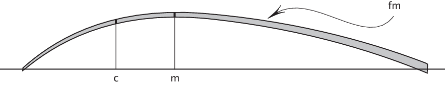
Consider vibrations of an inhomogeneous elastic string, either longitudinal or transversal, described by . Assume that the “stiffness coefficient” increases from left to right, just as in the last theorem. Then the the point of maximal amplitude of the fundamental mode lies between the “softest point ” and the thick end of the string. The same holds for any interval between two consecutive nodes of any overtone.
Figure 3 illustrates this effect for transversal oscillations.
Proof of the theorem. Let be the first eigenfunction of the operator (4):
| (11) |
which means that on and satisfies the homogeneous boundary conditions. We rewrite this relation as a system
| (12) |
Let us translate the definitions of and into geometrical terms. Since is defined by the condition (6), it is natural to choose (the resistance) as the new independent variable, so that (12) become
| (13) |
where and , . Assume without the loss of generality that
so that ranges in . Then is defined by
On the other hand, since is the maximizer of , we have , i.e. . Introducing the angle we restate the definition of as . Since is a monotone increasing function of , proving is equivalent to proving that . Since , the proof reduces to showing that
| (14) |

Now the angle satisfies
| (15) |
along with the boundary conditions and . Note that is a monotone increasing function and that for all values of its arguments, so that is monotone decreasing.
The key to the proof of (14) is the monotonicity of and the property . The idea is to compare the angle at equal times before and after crossing the zero value, as in Figure 4. That is, we introduce
| (16) |
so that . Moreover, these satisfy
| (17) |
where has been defined in (15). Since is monotone increasing, is monotone decreasing in and we have . Since , share the initial condition, the comparison theorem applies:
| (18) |
for , . Thus for some we have
or, recalling the definition of and :
By () we have
| (19) |
On the other hand, from the above we have , which implies (since and ). Adding this to (19) we obtain , thus completing the proof.
3 An open problem.
Consider a planar domain (Figure 5) bounded by two curves , where is a positive monotone increasing function, and by two lines . By symmetry, both points and lie on the –axis; let us denote by their –coordinates by and respectively.
Open problem 1: show that .
Open problem 2: show that for the Laplacian with mixed Dirichlet-Neumann boundary values: Dirichlet on , and Neumann on .

Remark. If we replace by with a small , then the membrane modeled by our mixed Dirichlet-Neumann problem becomes so narrow as to resemble an elastic string described in Theorem 2. This theorem in fact suggested the second open problem. For small our mixed Dirichlet-Neumann problem is approximated by the one–dimensional operator from Theorem 2. There is a vast literature on partial differential operators on thin domains; we refer to [4] and to references therein.
References
- [1] R. Courant and D. Hilbert. Methods of mathematical physics, Vol. 2. Interscience Publishers, 1989.
- [2] J. Denzler. Bounds for the heat diffusion through windows of given area. J. Math. Anal. Appl. 217, pages 405–422, 1998.
- [3] J. Denzler. Windows of given area with minimal heat diffusion. Trans. Amer. Math. Soc. v. 1, pages 569–580, 1999.
- [4] G. Raugel. Dynamics of partial differential equations on thin domains. Springer Lecture Notes in Mathematics V. 1609, 208-315, 1995.