Robust Nonparametric Regression via Sparsity Control
with Application to Load Curve Data Cleansing†
Abstract
Nonparametric methods are widely applicable to statistical inference problems, since they rely on a few modeling assumptions. In this context, the fresh look advocated here permeates benefits from variable selection and compressive sampling, to robustify nonparametric regression against outliers – that is, data markedly deviating from the postulated models. A variational counterpart to least-trimmed squares regression is shown closely related to an -(pseudo)norm-regularized estimator, that encourages sparsity in a vector explicitly modeling the outliers. This connection suggests efficient solvers based on convex relaxation, which lead naturally to a variational M-type estimator equivalent to the least-absolute shrinkage and selection operator (Lasso). Outliers are identified by judiciously tuning regularization parameters, which amounts to controlling the sparsity of the outlier vector along the whole robustification path of Lasso solutions. Reduced bias and enhanced generalization capability are attractive features of an improved estimator obtained after replacing the -(pseudo)norm with a nonconvex surrogate. The novel robust spline-based smoother is adopted to cleanse load curve data, a key task aiding operational decisions in the envisioned smart grid system. Computer simulations and tests on real load curve data corroborate the effectiveness of the novel sparsity-controlling robust estimators.
Index Terms:
Nonparametric regression, outlier rejection, sparsity, Lasso, splines, load curve cleansing.Submitted: August 24, 2026
EDICS Category: SSP-NPAR, MLR-LEAR.
I Introduction
Consider the classical problem of function estimation, in which an input vector is given, and the goal is to predict the real-valued scalar response . Function is unknown, to be estimated from a training data set . When is assumed to be a member of a finitely-parameterized family of functions, standard (non-)linear regression techniques can be adopted. If on the other hand, one is only willing to assume that belongs to a (possibly infinite dimensional) space of “smooth” functions , then a nonparametric approach is in order, and this will be the focus of this work.
Without further constraints beyond , functional estimation from finite data is an ill-posed problem. To bypass this challenge, the problem is typically solved by minimizing appropriately regularized criteria, allowing one to control model complexity; see, e.g., [12, 34]. It is then further assumed that has the structure of a reproducing kernel Hilbert space (RKHS), with corresponding positive definite reproducing kernel function , and norm denoted by . Under the formalism of regularization networks, one seeks as the solution to the variational problem
| (1) |
where is a convex loss function, and controls complexity by weighting the effect of the smoothness functional . Interestingly, the Representer Theorem asserts that the unique solution of (1) is finitely parametrized and has the form , where can be obtained from ; see e.g., [29, 38]. Further details on RKHS, and in particular on the evaluation of , can be found in e.g., [38, Ch. 1]. A fundamental relationship between model complexity control and generalization capability, i.e., the predictive ability of beyond the training set, was formalized in [37].
The generalization error performance of approaches that minimize the sum of squared model residuals [that is in (1)] regularized by a term of the form , is degraded in the presence of outliers. This is because the least-squares (LS) part of the cost is not robust, and can result in severe overfitting of the (contaminanted) training data [21]. Recent efforts have considered replacing the squared loss with a robust counterpart such as Huber’s function, or its variants, but lack a data-driven means of selecting the proper threshold that determines which datum is considered an outlier [43]; see also [27]. Other approaches have instead relied on the so-termed -insensitive loss function, originally proposed to solve function approximation problems using support vector machines (SVMs) [37]. These family of estimators often referred to as support vector regression (SVR), have been shown to enjoy robustness properties; see e.g., [32, 28, 26] and references therein. In [8], improved performance in the presence of outliers is achieved by refining the SVR solution through a subsequent robust learning phase.
The starting point here is a variational least-trimmed squares (VLTS) estimator, suitable for robust function approximation in (Section II). It is established that VLTS is closely related to an (NP-hard) -(pseudo)norm-regularized estimator, adopted to fit a regression model that explicitly incorporates an unknown sparse vector of outliers [17]. As in compressive sampling (CS) [35], efficient (approximate) solvers are obtained in Section III by replacing the outlier vector’s -norm with its closest convex approximant, the -norm. This leads naturally to a variational M-type estimator of , also shown equivalent to a least-absolute shrinkage and selection operator (Lasso) [33] on the vector of outliers (Section III-A). A tunable parameter in Lasso controls the sparsity of the estimated vector, and the number of outliers as a byproduct. Hence, effective methods to select this parameter are of paramount importance.
The link between -norm regularization and robustness was also exploited for parameter (but not function) estimation in [17] and [22]; see also [40] for related ideas in the context of face recognition, and error correction codes [4]. In [17] however, the selection of Lasso’s tuning parameter is only justified for Gaussian training data; whereas a fixed value motivated by CS error bounds is adopted in the Bayesian formulation of [22]. Here instead, a more general and systematic approach is pursued in Section III-B, building on contemporary algorithms that can efficiently compute all robustifaction paths of Lasso solutions, i.e., for all values of the tuning parameter [11, 16, 41]. In this sense, the method here capitalizes on but is not limited to sparse settings, since one can examine all possible sparsity levels along the robustification path. An estimator with reduced bias and improved generalization capability is obtained in Section IV, after replacing the -norm with a nonconvex surrogate, instead of the -norm that introduces bias [33, 44]. Simulated tests demonstrate the effectiveness of the novel approaches in robustifying thin-plate smoothing splines [10] (Section V-A), and in estimating the sinc function (Section V-B) – a paradigm typically adopted to assess performance of robust function approximation approaches [8, 43].
The motivating application behind the robust nonparametric methods of this paper is load curve cleansing [6] – a critical task in power systems engineering and management. Load curve data (also known as load profiles) refers to the electric energy consumption periodically recorded by meters at specific points across the power grid, e.g., end user-points and substations. Accurate load profiles are critical assets aiding operational decisions in the envisioned smart grid system [20]; see also [1, 2, 6]. However, in the process of acquiring and transmitting such massive volumes of information to a central processing unit, data is often noisy, corrupted, or lost altogether. This could be due to several reasons including meter misscalibration or outright failure, as well as communication errors due to noise, network congestion, and connectivity outages; see Fig. 1 for an example. In addition, data significantly deviating from nominal load models (outliers) are not uncommon, and could be attributed to unscheduled maintenance leading to shutdown of heavy industrial loads, weather constraints, holidays, strikes, and major sporting events, just to name a few.
In this context, it is critical to effectively reject outliers, and replace the contaminated data with ‘healthy’ load predictions, i.e., to cleanse the load data. While most utilities carry out this task manually based on their own personnel’s know-how, a first scalable and principled approach to load profile cleansing which is based on statistical learning methods was recently proposed in [6]; which also includes an extensive literature review on the related problem of outlier identification in time-series. After estimating the regression function via either B-spline or Kernel smoothing, pointwise confidence intervals are constructed based on . A datum is deemed as an outlier whenever it falls outside its associated confidence interval. To control the degree of smoothing effected by the estimator, [6] requires the user to label the outliers present in a training subset of data, and in this sense the approach therein is not fully automatic. Here instead, a novel alternative to load curve cleansing is developed after specializing the robust estimators of Sections III and IV, to the case of cubic smoothing splines (Section V-C). The smoothness-and outlier sparsity-controlling parameters are selected according to the guidelines in Section III-B; hence, no input is required from the data analyst. The proposed spline-based method is tested on real load curve data from a government building.
Concluding remarks are given in Section VI, while some technical details are deferred to the Appendix.
Notation: Bold uppercase letters will denote matrices, whereas bold lowercase letters will stand for column vectors. Operators , and will denote transposition, matrix trace and expectation, respectively; will be used for the cardinality of a set and the magnitude of a scalar. The norm of vector is for ; and is the matrix Frobenious norm. Positive definite matrices will be denoted by . The identity matrix will be represented by , while will denote the vector of all zeros, and .
II Robust Estimation Problem
The training data comprises noisy samples of taken at the input points (also known as knots in the splines parlance), and in the present context they can be possibly contaminated with outliers. Building on the parametric least-trimmed squares (LTS) approach [31], the desired robust estimate can be obtained as the solution of the following variational (V)LTS minimization problem
| (2) |
where is the -th order statistic among the squared residuals , and . In words, given a feasible , to evaluate the sum of the cost in (2) one: i) computes all squared residuals , ii) orders them to form the nondecreasing sequence ; and iii) sums up the smallest terms. As in the parametric LTS [31], the so-termed trimming constant (also known as coverage) determines the breakdown point of the VLTS estimator, since the largest residuals do not participate in (2). Ideally, one would like to make equal to the (typically unknown) number of outliers in the training data. For most pragmatic scenaria where is unknown, the LTS estimator is an attractive option due to its high breakdown point and desirable theoretical properties, namely -consistency and asymptotic normality [31].
The tuning parameter in (2) controls the tradeoff between fidelity to the (trimmed) data, and the degree of “smoothness” measured by . In particular, can be interpreted as a generalized ridge regularization term penalizing more those functions with large coefficients in a basis expansion involving the eigenfunctions of the kernel .
Given that the sum in (2) is a nonconvex functional, a nontrivial issue pertains to the existence of the proposed VLTS estimator, i.e., whether or not (2) attains a minimum in . Fortunately, a (conceptually) simple solution procedure suffices to show that a minimizer does indeed exist. Consider specifically a given subsample of training data points, say , and solve
A unique minimizer of the form is guaranteed to exist, where is used here to denote the chosen subsample, and the coefficients can be obtained by solving a particular linear system of equations [38, p. 11]. This procedure can be repeated for each subsample (there are of these), to obtain a collection of candidate solutions of (2). The winner(s) yielding the minimum cost, is the desired VLTS estimator. A remark is now in order.
Remark 1 (VLTS complexity)
Even though conceptually simple, the solution procedure just described guarantees existence of (at least) one solution, but entails a combinatorial search over all subsamples which is intractable for moderate to large sample sizes . In the context of linear regression, algorithms to obtain approximate LTS solutions are available; see e.g., [30].
II-A Robust function approximation via -norm regularization
Instead of discarding large residuals, the alternative approach proposed here explicitly accounts for outliers in the regression model. To this end, consider the scalar variables one per training datum, taking the value whenever datum adheres to the postulated nominal model, and otherwise. A regression model naturally accounting for the presence of outliers is
| (3) |
where are zero-mean independent and identically distributed (i.i.d.) random variables modeling the observation errors. A similar model was advocated under different assumptions in [17] and [22], in the context of robust parametric regression; see also [4] and [40]. For an outlier-free datum , (3) reduces to ; hence, will be often referred to as the nominal noise. Note that in (3), both as well as the vector are unknown; thus, (3) is underdetermined. On the other hand, as outliers are expected to often comprise a small fraction of the training sample say, not exceeding 20% – vector is typically sparse, i.e., most of its entries are zero; see also Remark 3. Sparsity compensates for underdeterminacy and provides valuable side-information when it comes to efficiently estimating , identifying outliers as a byproduct, and consequently performing robust estimation of the unknown function .
A natural criterion for controlling outlier sparsity is to seek the desired estimate as the solution of
| (4) |
where is a preselected threshold, and denotes the -norm of , which equals the number of nonzero entries of its vector argument. Sparsity is directly controlled by the selection of the tuning parameter . If the number of outliers were known a priori, then should be selected equal to . Unfortunately, analogously to related -norm constrained formulations in compressive sampling and sparse signal representations, problem (4) is NP-hard. In addition, (4) can be recast to an equivalent (unconstrained) Lagrangian form; see e.g., [3]
| (5) |
where the tuning Lagrange multiplier plays a role similar to in (4), and the -norm sparsity encouraging penalty is added to the cost.
To further motivate model (3) and the proposed criterion (5) for robust nonparametric regression, it is worth checking the structure of the minimizers of the cost in (5). Consider for the sake of argument that is given, and its value is such that , for some . The goal is to characterize , as well as the positions and values of the nonzero entries of . Note that because , the last term in (5) is constant, hence inconsequential to the minimization. Upon defining , it is not hard to see that the entries of satisfy
| (6) |
at the optimum. This is intuitive, since for those the best thing to do in terms of minimizing the overall cost is to set , and thus null the corresponding squared-residual terms in (5). In conclusion, for the chosen value of it holds that squared residuals effectively do not contribute to the cost in (5).
To determine the support of and , one alternative is to exhaustively test all admissible support combinations. For each one of these combinations (indexed by ), let be the index set describing the support of , i.e., if and only if ; and . By virtue of (6), the corresponding candidate minimizes
while is the one among all that yields the least cost. The previous discussion, in conjunction with the one preceding Remark 1 completes the argument required to establish the following result.
The importance of Proposition II-A is threefold. First, it formally justifies model (3) and its estimator (5) for robust function approximation, in light of the well documented merits of LTS regression [30]. Second, it further solidifies the connection between sparse linear regression and robust estimation. Third, the -norm regularized formulation in (5) lends itself naturally to efficient solvers based on convex relaxation, the subject dealt with next.
III Sparsity Controlling Outlier Rejection
To overcome the complexity hurdle in solving the robust regression problem in (5), one can resort to a suitable relaxation of the objective function. The goal is to formulate an optimization problem which is tractable, and whose solution yields a satisfactory approximation to the minimizer of the original hard problem. To this end, it is useful to recall that the -norm of vector is the closest convex approximation of . This property also utilized in the context of compressive sampling [35], provides the motivation to relax the NP-hard problem (5) to
| (7) |
Being a convex optimization problem, (7) can be solved efficiently. The nondifferentiable -norm regularization term controls sparsity on the estimator of , a property that has been recently exploited in diverse problems in engineering, statistics and machine learning. A noteworthy representative is the least-absolute shrinkage and selection operator (Lasso) [33], a popular tool in statistics for joint estimation and continuous variable selection in linear regression problems. In its Lagrangian form, Lasso is also known as basis pursuit denoising in the signal processing literature, a term coined by [7] in the context of finding the best sparse signal expansion using an overcomplete basis.
It is pertinent to ponder on whether problem (7) has built-in ability to provide robust estimates in the presence of outliers. The answer is in the affirmative, since a straightforward argument (details are deferred to the Appendix) shows that (7) is equivalent to a variational M-type estimator found by
| (8) |
where is a scaled version of Huber’s convex loss function [21]
| (9) |
Remark 2 (Regularized regression and robustness)
Existing works on linear regression have pointed out the equivalence between -norm regularized regression and M-type estimators, under specific assumptions on the distribution of the outliers (-contamination) [17, 23]. However, they have not recognized the link with LTS through the convex relaxation of (5), and the connection asserted by Proposition II-A. Here, the treatment goes beyond linear regression by considering nonparametric functional approximation in RKHS. Linear regression is subsumed as a special case, when the linear kernel is adopted. In addition, no assumption is imposed on the outlier vector.
It is interesting to compare the - and -norm formulations [cf. (5) and (7), respectively] in terms of their equivalent purely variational counterparts in (2) and (8), that entail robust loss functions. While the VLTS estimator completely discards large residuals, still retains them, but downweighs their effect through a linear penalty. Moreover, while (8) is convex, (2) is not and this has a direct impact on the complexity to obtain either estimator. Regarding the trimming constant in (2), it controls the number of residuals retained and hence the breakdown point of VLTS. Considering instead the threshold in Huber’s function , when the outliers’ distribution is known a-priori, its value is available in closed form so that the robust estimator is optimal in a well-defined sense [21]. Convergence in probability of M-type cubic smoothing splines estimators – a special problem subsumed by (8) – was studied in [9].
III-A Solving the convex relaxation
Because (7) is jointly convex in and , an alternating minimization (AM) algorithm can be adopted to solve (7), for fixed values of and . Selection of these parameters is a critical issue that will be discussed in Section III-B. AM solvers are iterative procedures that fix one of the variables to its most up to date value, and minimize the resulting cost with respect to the other one. Then the roles are reversed to complete one cycle, and the overall two-step minimization procedure is repeated for a prescribed number of iterations, or, until a convergence criterion is met. Letting denote iterations, consider that is fixed in (7). The update for at the -th iteration is given by
| (10) |
which corresponds to a standard regularization problem for functional approximation in [12], but with outlier-compensated data . It is well known that the minimizer of the variational problem (10) is finitely parameterized, and given by the kernel expansion [38]. The vector is found by solving the linear system of equations
| (11) |
where , and the matrix has entries .
In a nutshell, updating is equivalent to updating vector as per (11), where only the independent vector variable changes across iterations. Because the system matrix is positive definite, the per iteration systems of linear equations (11) can be efficiently solved after computing once, the Cholesky factorization of .
For fixed in (7), the outlier vector update at iteration is obtained as
| (12) |
where . Problem (12) can be recognized as an instance of Lasso for the so-termed orthonormal case, in particular for an identity regression matrix. The solution of such Lasso problems is readily obtained via soft-thresholding [15], in the form of
| (13) |
where is the soft-thresholding operator, and denotes the projection onto the nonnegative reals. The coordinatewise updates in (13) are in par with the sparsifying property of the norm, since for “small” residuals, i.e., , it follows that , and the -th training datum is deemed outlier free. Updates (11) and (13) comprise the iterative AM solver of the -norm regularized problem (7), which is tabulated as Algorithm 1. Convexity ensures convergence to the global optimum solution regardless of the initial condition; see e.g., [3].
Algorithm 1 is also conceptually interesting, since it explicitly reveals the intertwining between the outlier identification process, and the estimation of the regression function with the appropriate outlier-compensated data. An additional point is worth mentioning after inspection of (13) in the limit as . From the definition of the soft-thresholding operator , for those “large” residuals exceeding in magnitude, when , and otherwise. In other words, larger residuals that the method identifies as corresponding to outlier-contaminated data are shrunk, but not completely discarded. By plugging back into (7), these “large” residuals cancel out in the squared error term, but still contribute linearly through the -norm regularizer. This is exactly what one would expect, in light of the equivalence established with the variational -type estimator in (8).
Next, it is established that an alternative to solving a sequence of linear systems and scalar Lasso problems, is to solve a single instance of the Lasso with specific response vector and (non-orthonormal) regression matrix.
Proposition 2: Consider defined as
| (14) |
where
| (15) |
Then the minimizers of (7) are fully determined given , as and , with .
Proof:
For notational convenience introduce the vectors and , where is the minimizer of (7). Next, consider rewriting (7) as
| (16) |
The quantity inside the square brackets is a function of , and can be written explicitly after carrying out the minimization with respect to . From the results in [38], it follows that the vector of optimum predicted values at the points is given by ; see also the discussion after (10). Similarly, one finds that . Having minimized (16) with respect to , the quantity inside the square brackets is
| (17) |
After expanding the quadratic form in the right-hand side of (17), and eliminating the term that does not depend on , problem (16) becomes
Completing the square one arrives at
which completes the proof. ∎ The result in Proposition III-A opens the possibility for effective methods to select . These methods to be described in detail in the ensuing section, capitalize on recent algorithmic advances on Lasso solvers, which allow one to efficiently compute for all values of the tuning parameter . This is crucial for obtaining satisfactory robust estimates , since controlling the sparsity in by tuning is tantamount to controlling the number of outliers in model (3).
III-B Selection of the tuning parameters: robustification paths
As argued before, the tuning parameters and in (7) control the degree of smoothness in and the number of outliers (nonzero entries in ), respectively. From a statistical learning theory standpoint, and control the amount of regularization and model complexity, thus capturing the so-termed effective degrees of freedom [19]. Complex models tend to have worse generalization capability, even though the prediction error over the training set may be small (overfitting). In the contexts of regularization networks [12] and Lasso estimation for regression [33], corresponding tuning parameters are typically selected via model selection techniques such as cross-validation, or, by minimizing the prediction error over an independent test set, if available [19]. However, these simple methods are severely challenged in the presence of multiple outliers. For example, the swamping effect refers to a very large value of the residual corresponding to a left out clean datum , because of an unsatisfactory model estimation based on all data except ; data which contain outliers.
The idea here offers an alternative method to overcome the aforementioned challenges, and the possibility to efficiently compute for all values of , given . A brief overview of the state-of-the-art in Lasso solvers is given first. Several methods for selecting and are then described, which differ on the assumptions of what is known regarding the outlier model (3).
Lasso amounts to solving a quadratic programming (QP) problem [33]; hence, an iterative procedure is required to determine in (14) for a given value of . While standard QP solvers can be certainly invoked to this end, an increasing amount of effort has been put recently toward developing fast algorithms that capitalize on the unique properties of Lasso. The LARS algorithm [11] is an efficient scheme for computing the entire path of solutions (corresponding to all values of ), sometimes referred to as regularization paths. LARS capitalizes on piecewise linearity of the Lasso path of solutions, while incurring the complexity of a single LS fit, i.e., when . Coordinate descent algorithms have been shown competitive, even outperforming LARS when is large, as demonstrated in [16]; see also [42, 15], and the references therein. Coordinate descent solvers capitalize on the fact that Lasso can afford a very simple solution in the scalar case, which is given in closed form in terms of a soft-thresholding operation [cf. (13)]. Further computational savings are attained through the use of warm starts [15], when computing the Lasso path of solutions over a grid of decreasing values of . An efficient solver capitalizing on variable separability has been proposed in [41].
Consider then a grid of values of in the interval , evenly spaced in a logarithmic scale. Likewise, for each consider a similar type of grid consisting of values of , where is the minimum value such that [16], and in (14). Typically, with , say. Note that each of the values of gives rise to a different grid, since depends on through . Given the previously surveyed algorithmic alternatives to tackle the Lasso, it is safe to assume that (14) can be efficiently solved over the (nonuniform) grid of values of the tuning parameters. This way, for each value of one obtains samples of the Lasso path of solutions, which in the present context can be referred to as robustification path. As decreases, more variables enter the model signifying that more of the training data are deemed to contain outliers. An example of the robustification path is given in Fig. 3.
Based on the robustification paths and the prior knowledge available on the outlier model (3), several alternatives are given next to select the “best” pair in the grid .
Number of outliers is known: When is known, by direct inspection of the robustification paths one can determine the range of values for , for which has exactly nonzero entries. Specializing to the interval of interest, and after discarding outliers which are now fixed and known, -fold cross-validation methods can be applied to determine .
Variance of the nominal noise is known: Supposing that the variance of the i.i.d. nominal noise variables in (3) is known, one can proceed as follows. Using the solution obtained for each pair on the grid, form the sample variance matrix with -th entry
| (18) |
where stands for the number of nonzero entries in . Although not made explicit, the right-hand side of (18) depends on through the estimate , and . The entries correspond to a sample estimate of , without considering those training data that the method determined to be contaminated with outliers, i.e., those indices for which . The “winner” tuning parameters are such that
| (19) |
which is an absolute variance deviation (AVD) criterion.
Variance of the nominal noise is unknown: If is unknown, one can still compute a robust estimate of the variance , and repeat the previous procedure (with known nominal noise variance) after replacing with in (19). One option is based on the median absolute deviation (MAD) estimator, namely
| (20) |
where the residuals are formed based on a nonrobust estimate of , obtained e.g., after solving (7) with and using a small subset of the training dataset . The factor provides an approximately unbiased estimate of the standard deviation when the nominal noise is Gaussian. Typically, in (20) is used as an estimate for the scale of the errors in general M-type robust estimators; see e.g., [9] and [27].
Remark 3 (How sparse is sparse)
Even though the very nature of outliers dictates that is typically a small fraction of – and thus in (3) is sparse – the method here capitalizes on, but is not limited to sparse settings. For instance, choosing along the robustification paths allows one to continuously control the sparsity level, and potentially select the right value of for any given . Admittedly, if is large relative to , then even if it is possible to identify and discard the outliers, the estimate may not be accurate due to the lack of outlier-free data.
IV Refinement via Nonconvex Regularization
Instead of substituting in (5) by its closest convex approximation, namely , letting the surrogate function to be non-convex can yield tighter approximations. For example, the -norm of a vector was surrogated in [5] by the logarithm of the geometric mean of its elements, or by . In rank minimization problems, apart from the nuclear norm relaxation, minimizing the logarithm of the determinant of the unknown matrix has been proposed as an alternative surrogate [14]. Adopting related ideas in the present nonparametric context, consider approximating (5) by
| (21) |
where is a sufficiently small positive offset introduced to avoid numerical instability.
Since the surrogate term in (21) is concave, the overall problem is nonconvex. Still, local methods based on iterative linearization of , around the current iterate , can be adopted to minimize (21). From the concavity of the logarithm, its local linear approximation serves as a global overestimator. Standard majorization-minimization algorithms motivate minimizing the global linear overestimator instead. This leads to the following iteration for (see e.g., [25] for further details)
| (22) | ||||
| (23) |
It is possible to eliminate the optimization variable from (22), by direct application of the result in Proposition III-A. The equivalent update for at iteration is then given by
| (24) |
which amounts to an iteratively reweighted version of (14). If the value of is small, then in the next iteration the corresponding regularization term has a large weight, thus promoting shrinkage of that coordinate to zero. On the other hand when is significant, the cost in the next iteration downweighs the regularization, and places more importance to the LS component of the fit. For small , analysis of the limiting point of (24) reveals that
and hence, .
A good initialization for the iteration in (24) and (23) is , which corresponds to the solution of (14) [and (7)] for and . This is equivalent to a single iteration of (24) with all weights equal to unity. The numerical tests in Section V will indicate that even a single iteration of (24) suffices to obtain improved estimates , in comparison to those obtained from (14). The following remark sheds further light towards understanding why this should be expected.
Remark 4 (Refinement through bias reduction)
Uniformly weighted -norm regularized estimators such as (7) are biased [44], due to the shrinkage effected on the estimated coefficients. It will be argued next that the improvements due to (24) can be leveraged to bias reduction. Several workarounds have been proposed to correct the bias in sparse regression, that could as well be applied here. A first possibility is to retain only the support of (14) and re-estimate the amplitudes via, e.g., the unbiased LS estimator [11]. An alternative approach to reducing bias is through nonconvex regularization using e.g., the smoothly clipped absolute deviation (SCAD) scheme [13]. The SCAD penalty could replace the sum of logarithms in (21), still leading to a nonconvex problem. To retain the efficiency of convex optimization solvers while simultaneously limiting the bias, suitably weighted -norm regularizers have been proposed instead [44]. The constant weights in [44] play a role similar to those in (23); hence, bias reduction is expected.
V Numerical Experiments
V-A Robust thin-plate smoothing splines
To validate the proposed approach to robust nonparametric regression, a simulated test is carried out here in the context of thin-plate smoothing spline approximation [10, 39]. Specializing (7) to this setup, the robust thin-plate splines estimator can be formulated as
| (25) |
where denotes the Frobenius norm of the Hessian of . The penalty functional
| (26) |
extends to the one-dimensional roughness regularization used in smoothing spline models. For , the (non-unique) estimate in (25) corresponds to a rough function interpolating the outlier compensated data; while as the estimate is linear (cf. ). The optimization is over , the space of Sobolev functions, for which is well defined [10, p. 85]. Reproducing kernel Hilbert spaces such as , with inner-products (and norms) involving derivatives are studied in detail in [38].
Different from the cases considered so far, the smoothing penalty in (26) is only a seminorm, since first-order polynomials vanish under . Omitting details than can be found in [38, p. 30], under fairly general conditions a unique minimizer of (25) exists. The solution admits the finitely parametrized form , where in this case is a radial basis function. In simple terms, the solution as a kernel expansion is augmented with a member of the null space of . The unknown parameters are obtained in closed form, as solutions to a constrained, regularized LS problem; see [38, p. 33]. As a result, Proposition III-A still holds with minor modifications on the structure of .
Remark 5 (Bayesian framework)
Adopting a Bayesian perspective, one could model in (3) as a sample function of a zero mean Gaussian stationary process, with covariance function [24]. Consider as well that are mutually independent, while and in (3) are i.i.d. Gaussian and Laplace distributed, respectively. From the results in [24] and a straightforward calculation, it follows that setting and in (25) yields estimates (and ) which are optimal in a maximum a posteriori sense. This provides yet another means of selecting the parameters and , further expanding the options presented in Section III-B.
The simulation setup is as follows. Noisy samples of the true function comprise the training set . Function is generated as a Gaussian mixture with two components, with respective mean vectors and covariance matrices given by
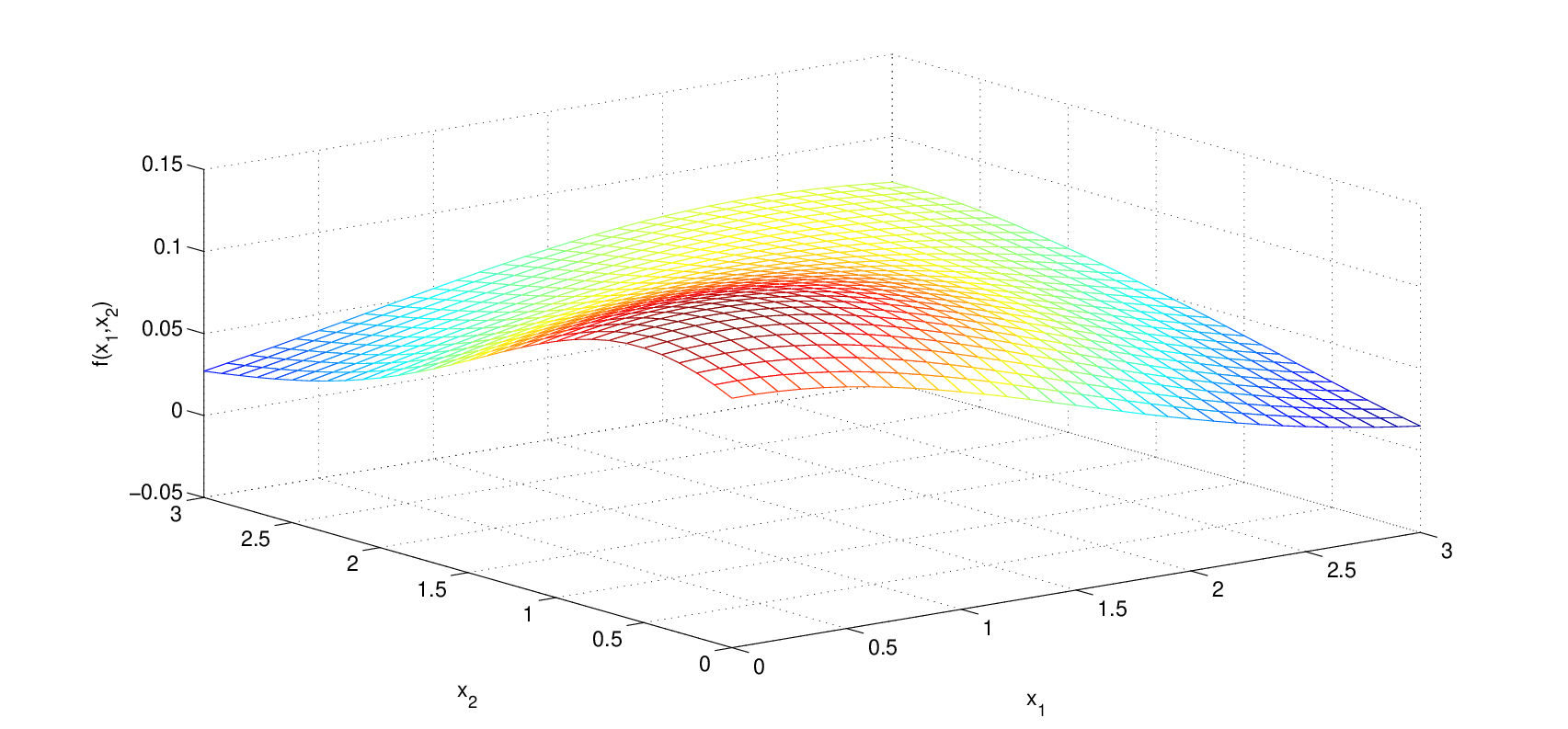
Function is depicted in Fig. 4 (a). The training data set comprises examples, with inputs drawn from a uniform distribution in the square . Several values ranging from to of the data are generated contaminated with outliers. Without loss of generality, the corrupted data correspond to the first training samples with , for which the response values are independently drawn from a uniform distribution over . Outlier-free data are generated according to the model , where the independent additive noise terms are Gaussian distributed, for . For the case where , the data used in the experiment is shown in Fig. 2. Superimposed to the true function are black points corresponding to data drawn from the nominal model, as well as red outlier points.
For this experiment, the nominal noise variance is assumed known. A nonuniform grid of and values is constructed, as described in Section III-B. The relevant parameters are , and . For each value of , the grid spans the interval defined by and , where . Each of the robustification paths corresponding to the solution of (14) is obtained using the SpaRSA toolbox in [41], exploiting warm starts for faster convergence. Fig. 3 depicts an example with and . With the robustification paths at hand, it is possible to form the sample variance matrix [cf. (18)], and select the optimum tuning parameters based on the criterion (19). Finally, the robust estimates are refined by running a single iteration of (24) as described in Section IV. The value was utilized, and several experiments indicated that the results are quite insensitive to the selection of this parameter.
The same experiment was conducted for a variable number of outliers , and the results are listed in Table I. In all cases, a outlier identification success rate was obtained, for the chosen value of the tuning parameters. This even happened at the first stage of the method, i.e., in (14) had the correct support in all cases. It has been observed in some other setups that (14) may select a larger support than , but after running a few iterations of (24) the true support was typically identified. To assess quality of the estimated function , two figures of merit were considered. First, the training error was evaluated as
i.e., the average loss over the training sample after excluding outliers. Second, to assess the generalization capability of , an approximation to the generalization error was computed as
| (27) |
where is an independent test set generated from the model . For the results in Table I, was adopted corresponding to a uniform rectangular grid of points in . Inspection of Table I reveals that the training errors are comparable for the function estimates obtained after solving (7) or its nonconvex refinement (21). Interestingly, when it comes to the more pragmatic generalization error , the refined estimator (21) has an edge for all values of . As expected, the bias reduction effected by the iteratively reweighting procedure of Section IV improves considerably the generalization capability of the method; see also Remark 4.
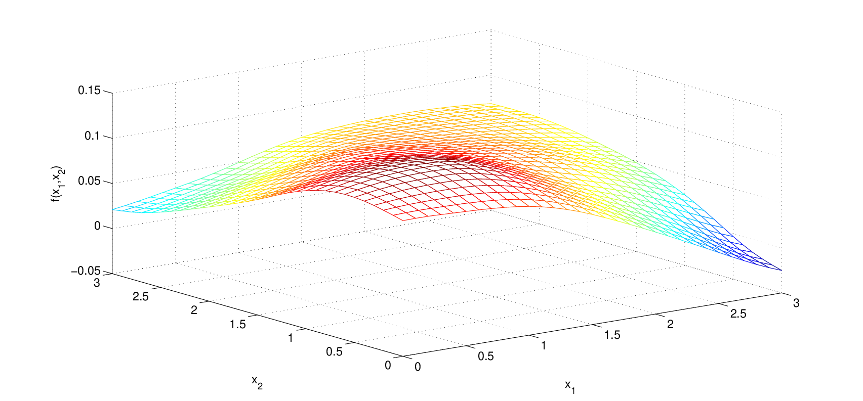
A pictorial summary of the results is given in Fig 4, for outliers. Fig 4 (a) depicts the true Gaussian mixture , whereas Fig. 4 (b) shows the nonrobust thin-plate splines estimate obtained after solving
| (28) |
Even though the thin-plate penalty enforces some degree of smoothness, the estimate is severely disrupted by the presence of outliers [cf. the difference on the -axis ranges]. On the other hand, Figs. 4 (c) and (d), respectively, show the robust estimate with , and its bias reducing refinement. The improvement is apparent, corroborating the effectiveness of the proposed approach.
V-B Sinc function estimation
| Method | |||
|---|---|---|---|
| Nonrobust [(1) with ] | |||
| SVR with | |||
| RSVR with | |||
| SVR with | |||
| RSVR with | |||
| Sparsity-controlling in (7) | |||
| Refinement in (21) |
The univariate function is commonly adopted to evaluate the performance of nonparametric regression methods [8, 43]. Given noisy training examples with a small fraction of outliers, approximating over the interval is considered in the present simulated test. The sparsity-controlling robust nonparametric regression methods of this paper are compared with the SVR [37] and robust SVR in [8], for the case of the -insensitve loss function with values and . In order to implement (R)SVR, routines from a publicly available SVM Matlab toolbox were utilized [18]. Results for the nonrobust regularization network approach in (1) (with ) are reported as well, to assess the performance degradation incurred when compared to the aforementioned robust alternatives. Because the fraction of outliers () in the training data is assumed known to the method of [8], the same will be assumed towards selecting the tuning parameters and in (7), as described in Section III-B. The -grid parameters selected for the experiment in Section V-A were used here as well, except for . Space is chosen to be the RKHS induced by the positive definite Gaussian kernel function , with parameter for all cases.
The training set comprises examples, with scalar inputs drawn from a uniform distribution over . Uniformly distributed outliers are artificially added in , with resulting in contamination. Nominal data in adheres to the model for , where the independent additive noise terms are zero-mean Gaussian distributed. Three different values are considered for the nominal noise variance, namely for . For the case where , the data used in the experiment are shown in Fig. 5 (a). Superimposed to the true function (shown in blue) are black points corresponding to the noisy data obeying the nominal model, as well as outliers depicted as red points.
The results are summarized in Table II, which lists the generalization errors attained by the different methods tested, and for varying . The independent test set used to evaluate (27) was generated from the model , where the define a -element uniform grid over . A first (expected) observation is that all robust alternatives markedly outperform the nonrobust regularization network approach in (1), by an order of magnitude or even more, regardless of the value of . As reported in [8], RSVR uniformly outperforms SVR. For the case , RSVR also uniformly outperforms the sparsity-controlling method in (7). Interestingly, after refining the estimate obtained via (7) through a couple iterations of (24) (cf. Section IV), the lowest generalization errors are obtained, uniformly across all simulated values of the nominal noise variance. Results for the RSVR with come sufficiently close, and are equally satisfactory for all practical purposes; see also Fig. 5 for a pictorial summary of the results when .
While specific error values or method rankings are arguably anecdotal, two conclusions stand out: (i) model (3) and its sparsity-controlling estimators (7) and (21) are effective approaches to nonparametric regression in the presence of outliers; and (ii) when initialized with the refined estimator (21) can considerably improve the performance of (7), at the price of a modest increase in computational complexity. While (7) endowed with the sparsity-controlling mechanisms of Section III-B tends to overestimate the “true” support of , numerical results have consistently shown that the refinement in Section IV is more effective when it comes to support recovery.
V-C Load curve data cleansing
In this section, the robust nonparametric methods described so far are applied to the problem of load curve cleansing outlined in Section I. Given load data corresponding to a building’s power consumption measurements , acquired at time instants , , the proposed approach to load curve cleansing minimizes
| (29) |
where denotes the second-order derivative of . This way, the solution provides a cleansed estimate of the load profile, and the support of indicates the instants where significant load deviations, or, meter failures occurred. Estimator (29) specializes (7) to the so-termed cubic smoothing splines; see e.g., [19, 38]. It is also subsumed as a special case of the robust thin-plate splines estimator (25), when the target function has domain in [cf. how the smoothing penalty (26) simplifies to the one in (29) in the one-dimensional case].
In light of the aforementioned connection, it should not be surprising that admits a unique, finite-dimensional minimizer, which corresponds to a natural spline with knots at ; see e.g., [19, p. 151]. Specifically, it follows that , where is the basis set of natural spline functions, and the vector of expansion coefficients is given by
where matrix has -th entry ; while has -th entry . Spline coefficients can be computed more efficiently if the basis of B-splines is adopted instead; details can be found in [19, p. 189] and [36].
Without considering the outlier variables in (29), a B-spline estimator for load curve cleansing was put forth in [6]. An alternative Nadaraya-Watson estimator from the Kernel smoothing family was considered as well. In any case, outliers are identified during a post-processing stage, after the load curve has been estimated nonrobustly. Supposing for instance that the approach in [6] correctly identifies outliers most of the time, it still does not yield a cleansed estimate . This should be contrasted with the estimator (29), which accounts for the outlier compensated data to yield a cleansed estimate at once. Moreover, to select the “optimum” smoothing parameter , the approach of [6] requires the user to manually label the outliers present in a training subset of data, during a pre-processing stage. This subjective component makes it challenging to reproduce the results of [6], and for this reason comparisons with the aforementioned scheme are not included in the sequel.
Next, estimator (29) is tested on real load curve data provided by the NorthWrite Energy Group. The dataset consists of power consumption measurements (in kWh) for a government building, collected every fifteen minutes during a period of more than five years, ranging from July 2005 to October 2010. Data is downsampled by a factor of four, to yield one measurement per hour. For the present experiment, only a subset of the whole data is utilized for concreteness, where was chosen corresponding to a hour period. A snapshot of this training load curve data in , spanning a particular three-week period is shown in Fig. 6 (a). Weekday activity patterns can be clearly discerned from those corresponding to weekends, as expected for most government buildings; but different, e.g., for the load profile of a grocery store. Fig. 6 (b) shows the nonrobust smoothing spline fit to the training data in (also shown for comparison purposes), obtained after solving
| (30) |
using Matlab’s built-in spline toolbox. Parameter was chosen based on leave-one-out cross-validation, and it is apparent that no cleansing of the load profile takes place. Indeed, the resulting fitted function follows very closely the training data, even during the abnormal energy peaks observed on the so-termed “building operational transition shoulder periods.”
Because with real load curve data the nominal noise variance in (3) is unknown, selection of the tuning parameters in (29) requires a robust estimate of the variance such as the MAD [cf. Section III-B]. Similar to [6], it is assumed that the nominal errors are zero mean Gaussian distributed, so that (20) can be applied yielding the value . To form the residuals in (20), (30) is solved first using a small subset of that comprises measurements. A nonuniform grid of and values is constructed, as described in Section III-B. Relevant parameters are , , , , and . The robustification paths (one per value in the grid) were obtained using the SpaRSA toolbox in [41], with the sample variance matrix formed as in (18). The optimum tuning parameters and are finally determined based on the criterion (19), where the unknown is replaced with . Finally, the cleansed load curve is refined by running four iterations of (24) as described in Section IV, with a value of . Results are depicted in Fig. 7, where the cleansed load curves are superimposed to the training data in . Red circles indicate those data points deemed as outliers, information that is readily obtained from the support of . By inspection of Fig. 7, it is apparent that the proposed sparsity-controlling estimator has the desired cleansing capability. The cleansed load curves closely follow the training data, but are smooth enough to avoid overfitting the abnormal energy peaks on the “shoulders.” Indeed, these peaks are in most cases identified as outliers. As seen from Fig. 7 (a), the solution of (29) tends to overestimate the support of , since one could argue that some of the red circles in Fig. 7 (a) do not correspond to outliers. Again, the nonconvex regularization in Section IV prunes the outlier support obtained via (29), resulting in a more accurate result and reducing the number of outliers identified from to .
VI Concluding Summary
Outlier-robust nonparametric regression methods were developed in this paper for function approximation in RKHS. Building on a neat link between the seemingly unrelated fields of robust statistics and sparse regression, the novel estimators were found rooted at the crossroads of outlier-resilient estimation, the Lasso, and convex optimization. Estimators as fundamental as LS for linear regression, regularization networks, and (thin-plate) smoothing splines, can be robustified under the proposed framework.
Training samples from the (unknown) target function were assumed generated from a regression model, which explicitly incorporates an unknown sparse vector of outliers. To fit such a model, the proposed variational estimator minimizes a tradeoff between fidelity to the training data, the degree of “smoothness” of the regression function, and the sparsity level of the vector of outliers. While model complexity control effected through a smoothing penalty has quite well understood ramifications in terms of generalization capability, the major innovative claim here is that sparsity control is tantamount to robustness control. This is indeed the case since a tunable parameter in a Lasso reformulation of the variational estimator, controls the degree of sparsity in the estimated vector of model outliers. Selection of tuning parameters could be at first thought as a mundane task. However, arguing on the importance of such task in the context of robust nonparametric regression, as well as devising principled methods to effectively carry out smoothness and sparsity control, are at the heart of this paper’s novelty. Sparsity control can be carried out at affordable complexity, by capitalizing on state-of-the-art algorithms that can efficiently compute the whole path of Lasso solutions. In this sense, the method here capitalizes on but is not limited to sparse settings where few outliers are present, since one can efficiently examine the gamut of sparsity levels along the robustification path. Computer simulations have shown that the novel methods of this paper outperform existing alternatives including SVR, and one if its robust variants.
As an application domain relevant to robust nonparametric regression, the problem of load curve cleansing for power systems engineering was also considered along with a solution proposed based on robust cubic spline smoothing. Numerical tests on real load curve data demonstrated that the smoothness and sparsity controlling methods of this paper are effective in cleansing load profiles, without user intervention to aid the learning process.
Acknowledgment
The authors would like to thank NorthWrite Energy Group and Prof. Vladimir Cherkassky (Dept. of ECE, University of Minnesota) for providing the load curve data analysed in Section V-C.
Towards establishing the equivalence between problems (7) and (8), consider the pair that solves (7). Assume that is given, and the goal is to determine . Upon defining the residuals and because , the entries of are separately given by
| (31) |
where the term in (7) has been omitted, since it is inconsequential for the minimization with respect to . For each , because (31) is nondifferentiable at the origin one should consider three cases: i) if , it follows that the minimum cost in (31) is ; ii) if , the first-order condition for optimality gives provided , and the minimum cost is ; otherwise, iii) if , it follows that provided , and the minimum cost is . In other words,
| (32) |
Upon plugging (32) into (31), the minimum cost in (31) after minimizing with respect to is [cf. (9) and the argument preceding (32)]. All in all, the conclusion is that is the minimizer of (8) – in addition to being the solution of (7) by definition – completing the proof.
References
- [1] Energy Independence and Security Act of 2007, an Act of the Congress of the United States of America Publ. L. No. 110-140, H.R. 6, Dec. 2007.
- [2] The Smart Grid: An Introduction, United States Department of Energy, Office of Electricity Delivery and Energy Reliability, Jan. 2010. [Online]. Available: http://www.oe.energy.gov/1165.htm
- [3] D. P. Bertsekas, Nonlinear Programming, 2nd ed. Athena-Scientific, 1999.
- [4] E. J. Candes and P. A. Randall, “Highly robust error correction by convex programming,” IEEE Trans. on Inf. Theory, vol. 54, no. 7, pp. 2829–2840, 2008.
- [5] E. J. Candes, M. B. Wakin, and S. Boyd, “Enhancing sparsity by reweighted minimzation,” Journal of Fourier Analysis and Applications, vol. 14, pp. 877–905, Dec. 2008.
- [6] J. Chen, W. Li, A. Lau, J. Cao, and K. Eang, “Automated load curve data cleansing in power systems,” IEEE Trans. Smart Grid, vol. 1, pp. 213–221, Sep. 2010.
- [7] S. S. Chen, D. L. Donoho, and M. A. Saunders, “Atomic decomposition by basis pursuit,” SIAM Journal on Scientific Computing, vol. 20, pp. 33–61, 1998.
- [8] C. C. Chuang, S. F. Fu, J. T. Jeng, and C. C. Hsiao, “Robust support vector regression networks for function approximation with outliers,” IEEE Trans. Neural Netw., vol. 13, pp. 1322–1330, Jun. 2002.
- [9] D. D. Cox, “Asymptotics for M-type smoothing splines,” Ann. Statist., vol. 11, pp. 530–551, 1983.
- [10] J. Duchon, Splines Minimizing Rotation-Invariant Semi-norms in Sobolev Spaces. Springer-Verlag, 1977.
- [11] B. Efron, T. Hastie, I. M. Johnstone, and R. Tibshirani, “Least angle regression,” Ann. Statist., vol. 32, pp. 407–499, 2004.
- [12] T. Evgeniou, M. Pontil, and T. Poggio, “Regularization networks and support vector machines,” Advances in Computational Mathematics, vol. 13, pp. 1–50, 2000.
- [13] J. Fan and R. Li, “Variable selection via nonconcave penalized likelihood and its oracle properties,” J. Amer. Stat. Assoc., vol. 96, pp. 1348–1360, 2001.
- [14] M. Fazel, “Matrix rank minimization with applications,” Ph.D. dissertation, Stanford University, 2002.
- [15] J. Friedman, T. Hastie, H. Hofling, and R. Tibshirani, “Pathwise coordinate optimization,” Ann. Appl. Stat., vol. 1, pp. 302–332, 2007.
- [16] J. Friedman, T. Hastie, and R. Tibshirani, “Regularized paths for generalized linear models via coordinate descent,” Journal of Statistical Software, vol. 33, 2010.
- [17] J. J. Fuchs, “An inverse problem approach to robust regression,” in Proc. of Intl. Conf. on Acoustics, Speech and Signal Processing, Phoeniz, AZ, Mar. 1999, pp. 180–188.
- [18] S. R. Gunn, Matlab SVM Toolbox, 1997. [Online]. Available: http://www.isis.ecs.soton.ac.uk/resources/svminfo/
- [19] T. Hastie, R. Tibshirani, and J. Friedman, The Elements of Statistical Learning, 2nd ed. Springer, 2009.
- [20] S. G. Hauser, vision for the smart grid, presented at the U.S. Department of Energy Smart Grid R&D Roundtable Meeting, Dec. 9, 2009.
- [21] P. J. Huber and E. M. Ronchetti, Robust Statistics. New York: Wiley, 2009.
- [22] Y. Jin and B. D. Rao, “Algorithms for robust linear regression by exploiting the connection to sparse signal recovery,” in Proc. of Intl. Conf. on Acoustics, Speech and Signal Processing, Dallas, TX, Mar. 2010, pp. 3830–3833.
- [23] V. Kekatos and G. B. Giannakis, “From sparse signals to sparse residuals for robust sensing,” IEEE Trans. Signal Process., vol. 59, 2011 (to appear); http://spincom.umn.edu/journal.html.
- [24] G. Kimbeldorf and G. Wahba, “A correspondence between bayesian estimation on stochastic processes and smoothing by splines,” Ann. Math. Statist., vol. 41, pp. 495–502, 1970.
- [25] K. Lange, D. Hunter, and I. Yang, “Optimization transfer using surrogate objective functions (with discussion),” J. Computat. Graph. Statist., vol. 9, pp. 1–59, 2000.
- [26] Y. J. Lee, W. F. Heisch, and C. M. Huang, “-SSVR: A smooth support vector machine for -insensitive regression,” IEEE Trans. Knowl. Data Eng., vol. 17, pp. 678–685, 2005.
- [27] O. L. Mangasarian and D. R. Musicant, “Robust linear and support vector regression,” IEEE Trans. Pattern Anal. Mach. Intell., vol. 22, pp. 950–955, Sep. 2000.
- [28] S. Mukherjee, E. Osuna, and F. Girosi, “Nonlinear prediction of chaotic time series using a support vector machine,” in Proc. of Wrkshp. Neural Networks for Signal Proces., Amelia Island, FL, 97, pp. 24–26.
- [29] T. Poggio and F. Girosi, “A theory of networks for approximation and learning,” A. I. Memo No. 1140, Artificial Intelligence Laboratory, Massachussets Institute of Technology, 1989.
- [30] P. J. Rousseeuw and K. V. Driessen, “Computing LTS regression for large data sets,” Data Mining and Knowledge Discovery, vol. 12, pp. 29–45, 2006.
- [31] P. J. Rousseeuw and A. M. Leroy, Robust regression and outlier detection. New York: Wiley, 1987.
- [32] A. J. Smola and B. Scholkopf, “A tutorial on support vector regression,” Neuro COLT Technical Report TR-1998-030, Royal Holloway College, London, 1998.
- [33] R. Tibshirani, “Regression shrinkage and selection via the lasso,” J. Royal. Statist. Soc B, vol. 58, pp. 267–288, 1996.
- [34] A. N. Tikhonov and V. Y. Arsenin, Solutions of Ill-posed Problems. Washington, DC: W. H. Winston, 1977.
- [35] J. Tropp, “Just relax: Convex programming methods for identifying sparse signals,” IEEE Trans. Inf. Theory, vol. 51, pp. 1030–1051, Mar. 2006.
- [36] M. Unser, “Splines: A perfect fit for signal and image processing,” IEEE Signal Processing Magazine, vol. 16, pp. 22–38, Nov. 1999.
- [37] V. Vapnik, Statistical Learning Theory. New York: Wiley, 1998.
- [38] G. Wahba, Spline Models for Observational Data. Philadelphia: SIAM, 1990.
- [39] G. Wahba and J. Wendelberger, “Some new mathematical methods for variational objective analysis using splines and cross validation,” Monthly Weather Review, vol. 108, pp. 1122–1145, 1980.
- [40] J. Wright and Y. Ma, “Dense error correction via -minimization,” IEEE Trans. Inf. Theory, vol. 56, no. 7, pp. 3540–3560, 2010.
- [41] S. J. Wright, R. D. Nowak, and M. A. T. Figueiredo, “Sparse reconstruction by separable approximation,” IEEE Trans. Signal Process., vol. 57, pp. 2479–2493, 2009.
- [42] T. Wu and K. Lange, “Coordinate descent algorithms for lasso penalized regression,” Ann. Appl. Stat., vol. 2, pp. 224–244, 2008.
- [43] J. Zhu, S. C. H. Hoi, and M. R. T. Lyu, “Robust regularized kernel regression,” IEEE Trans. Syst., Man, Cybern. B Cybern., vol. 38, pp. 1639–1644, Dec. 2008.
- [44] H. Zou, “The adaptive Lasso and its oracle properties,” J. Amer. Stat. Assoc., vol. 101, no. 476, pp. 1418–1429, 2006.


(a)

(b)
(c)

(d)

(a)

(b)

(c)

(d)

(e)

(f)

(g)

(h)

(a)

(b)

(a)

(b)