Effective Field Theory of Fractional Quantized Hall Nematics
Abstract
We present a Landau-Ginzburg theory for a fractional quantized Hall nematic state and the transition to it from an isotropic fractional quantum Hall state. This justifies Lifshitz-Chern-Simons theory – which is shown to be its dual – on a more microscopic basis and enables us to compute a ground state wave function in the symmetry-broken phase. In such a state of matter, the Hall resistance remains quantized while the longitudinal DC resistivity due to thermally-excited quasiparticles is anisotropic. We interpret recent experiments at Landau level filling factor in terms of our theory.
Introduction.
A fractional quantized Hall nematic (FQHN) is a phase in which a fractional quantized Hall conductance coexists with the broken rotational symmetry characteristic of a nematic, as in the model introduced in Ref. 1. The idea that a phase of matter could have both topological order and conventional broken symmetry is not new; for instance, quantum Hall ferromagnets are another example [2, 3]. See [4] for a more recent discussion in a related system. However, the FQHN has the unusual feature that the broken symmetry and the topological order are equally important for determining the system’s transport properties. Furthermore, the model also predicts an unusual quantum critical point separating the FQHN from an ordinary isotropic fractional quantum Hall state.
Remarkably, a recent experiment may have observed a FQHN [5]. An in-plane magnetic field is applied to the fractional quantum Hall plateau. When the angle between the total magnetic field and the normal is zero, the system is essentially isotropic: for mK, . At mK, there is a well-developed Hall plateau with . At mK, there is a small () difference between and , which may be due to device geometry, alignment of the contacts, or a small intrinsic anisotropy acquired by the samples during the growth process. For tilt angles and mK, while increases with decreasing temperature. In fact, while at the lowest observed temperatures. Thus, this experiment finds transport which is reminiscent of the nematic phases found at half-filling of higher Landau levels, such as without an in-plane field [6, 7] and also at and in the presence of an in-plane field [8, 9], except for one very striking difference: the Hall resistance remains quantized in the anisotropic phase.
We interpret these observations as a slightly rounded transition between an isotropic fractional quantum Hall phase at and an FQHN at . The rounding of the transition is caused by the in-plane field. We believe it to be a weak rotational symmetry-breaking field because the system is in an isotropic metallic phase for even larger tilts at the nearby fraction [10] and because the anisotropy at 300 mK actually decreases as the tilt is increased from to . We conjecture that the most important effect of the in-plane field is to vary the effective interaction between the electrons, thereby driving the (almost) spontaneous breaking of rotational symmetry. We are thus led to apply our model [1] to this experiment.
To this end, we give a more microscopic derivation of our model as a Landau-Ginzburg theory. We thereby recover a theory which is equivalent, through particle-vortex duality, to the effective field theory introduced in Ref. 1. In order to compare theory and experiment more closely, we extend our previous analysis of zero-temperature, finite-frequency transport to finite-temperature DC transport; in order to do this, we must enlarge our model to include the effects of gapped charged quasiparticles. The development of nematic order induces strongly temperature-dependent anisotropy in the quasiparticle effective masses. We predict that both longitudinal conductances will eventually vanish at the lowest temperatures, although one of them will have non-monotonic temperature dependence at slightly higher temperatures. We finally make predictions for transport at and near the transition point.
Landau-Ginzburg Theory.
One can map the problem of spinless planar electrons in a transverse magnetic field with Coulomb repulsion, to an equivalent system of a bosonic order parameter of unit charge coupled to a Chern-Simons gauge field [11]. The action takes the form:
| (1) | |||||
| (2) | |||||
| (3) |
is the background electromagnetic field satisfying ; is the mean charge density of bosons (or equivalently, electrons); is the electron band mass; V(x) is a general two-body potential; and the Chern-Simons gauge field attaches units of statistical flux to each particle [12]. In particular, for an odd integer, the resulting Aharonov-Bohm phases transmute the bosons into fermions.
We assume that the low-energy effective theory for distances longer than the magnetic length, obtained by integrating out short-distance fluctuations of , , has the same form as the microscopic action (1), but with the bare microscopic parameters and replaced by renormalized ones, and . Such an ansatz allows one to derive many of the properties of the standard fractional quantum Hall states [11, 13]. Here, we will make the same ansatz, but without assuming that remains positive. We note that even the ‘microscopic’ action (1) must be viewed as an effective low-energy action that describes the partially filled Landau level with . The electrons are confined to a quantum well of finite-width; a strictly two-dimensional theory is an effective theory at energy scales far below the splitting between energy sub-bands for motion perpendicular to the plane. Thus, the application of the in-plane field , through its modification of the motion perpendicular to the plane, will modify the parameters in . Consequently, the effective parameters at distances longer than the magnetic length will also be modified, but not in a simple or, at present, transparent way. It is easy to check that reasonable local variations of do not cause qualitative changes to the physics of (1) [13]. We leave to a future study the question of higher-body potential terms resulting from a projection of the degrees of freedom into a specific Landau level.
Therefore, we conjecture that as the in-plane field is varied, the most significant variation is of the parameter . In other words, we study the instabilities of (1) as the kinetic structure of the theory is modified.
Since we will be considering , we add the following term with to the action in order to maintain stability of the vacuum:
| (4) |
This theory exhibits a transition between an isotropic fractional quantum Hall phase, when , and an anisotropic phase with well-quantized Hall conductance (after inclusion of disorder or a lattice) when , just as in [1]. The two phases are separated by a quantum critical point with dynamical scaling, arising at .
Kohn’s Theorem.
On might object to any variation of from its bare value on the basis of Kohn’s theorem [14]. (See Section 5 of [13] for a discussion.) In a Galilean-invariant system of identical mutually interacting particles of unit charge and mass subject to a constant external magnetic field , Kohn’s theorem states that the density-density correlation function has the low momentum limit,
| (5) |
The locations of the two poles are determined by the cyclotron frequency . For fixed , the cyclotron frequency is determined by the bare mass of the particles, independent of the their relative interactions. The residues of the poles are equal to . The form of this correlator is ensured by a Ward identity and satisfies an f-sum rule. Kohn’s theorem roughly states that the center-of-mass of the system always decouples from the relative coordinate motion of the particles; it effectively behaves as a single charge particle of mass , exhibiting circular motion at a frequency in a background magnetic field . In quantum Hall systems, the quantum well explicitly breaks translational symmetry in the -direction (i.e. perpendicular to the plane). However, the in-plane center-of-mass motion still decouples from the other degrees of freedom, so long as the magnetic field is strictly perpendicular to the plane. Thus, Kohn’s theorem holds even in this case.
If we now compute the density-density correlator using the action (1), we find precisely the form dictated by Kohn’s theorem (5). However, the modification would change the location of the pole. This manifestly constitutes a violation of Kohn’s theorem.
However, the experiment of Ref. 5 does not satisfy the assumptions of Kohn’s theorem. The large in-plane field, combined with the confining well potential (perpendicular to the plane), manifestly breaks Galilean invariance and does not allow a decoupling of the center-of-mass mode. The in-plane field couples motion along the -direction to motion in the plane, while the confining potential in the -direction couples the -component of the center-of-mass position to the -component of the relative coordinates. The Landau level in the devices considered in Ref. 5 is particularly susceptible to perturbations mixing planar and -direction motion because the gap to the Landau level of the next quantum well sub-band is small [10].
In summary, our theory, in which is not fixed, applies to situations, such as those in the experiment of Ref. 5, in which Kohn’s theorem does not hold. Our theory cannot describe a fictional system in which the two-dimensional layer is infinitely-thin and the transition is driven purely by tuning the inter-electron interaction (without any in-plane field) since such a system would necessarily satisfy Kohn’s theorem. To make our point more concrete, we show in the Appendix that, as a result of the violation of the conditions of Kohn’s theorem, the location of the cyclotron pole can vary as is increased.
Duality.
We have computed the long wavelength transport properties of the various phases of (1) directly from the Landau-Ginzburg theory and found them to exactly match the response determined from the Lifshitz-Chern-Simons (LCS) theory of [1]. This is expected because there is a low-energy equivalence between the (more) microscopic theory (1), (4) and the LCS theory which we demonstrate by expanding about the relevant ground state in the three cases , and mapping the low-energy theory to the action governing the similar phase of the LCS theory, using particle-vortex duality [15]. For convenience, we assume a short-ranged repulsive interaction, with , throughout. This choice is motivated by expected screening effects of the microscopic electrons. Nevertheless, the precise form of plays very little role in the considerations below as long as it is local.
For , there is a saddle point configuration given by , , with filling fraction . The low-energy action for fluctuations about this ground state when is
| (6) | |||||
| (7) |
and govern the fluctuations of the norm and phase of the bosonic order parameter , represents the fluctuation of the Chern-Simons gauge field, and we have taken the background field fluctuations to vanish. can be rewritten by introducing the field (the spatial components of the current associated with the background gauge field):
| (8) | |||||
| (9) |
Now, integrating out trivially reproduces the previous Lagrangian; but we can instead find a dual description of the theory by keeping in the Lagrangian and integrating out the other degrees of freedom. appears linearly and functions as a Lagrange multiplier ensuring conservation of . We can guarantee this by rewriting . Writing the theory in terms of , and integrating out , we find
| (10) | |||
| (11) |
This is Maxwell-Chern-Simons theory at level with and . This matches the behavior of the LCS theory of [1] in the fractional quantum Hall phase .
When (the critical point), it is necessary to keep the term. Nevertheless, the dualization proceeds almost identically. The leading terms in the expansion of the action in small fluctuations about the saddle point are
| (12) |
This is a formal expression because of the inverse Laplacian in the second term. Current conservation, which is imposed by the equation of motion, allows us to replace with the emergent gauge field . Imposing the gauge conditions and , and integrating out , we obtain a gauge-fixed version of the LCS Lagrangian. Covariantizing the gauge-fixed action yields
| (13) | |||
| (14) |
where , and . This is precisely the theory governing the critical point in [1], with the field integrated out. (The nature of the field action in that theory, gives rise to the peculiar inverse Laplacian in the action above).
Lastly, we discuss the anisotropic phase. The ground state is still homogeneous, , but anisotropic, since , with, and . At this saddle point, the chemical potential is shifted upwards. The leading terms in the low-energy action, expanding around the symmetry-breaking vacuum with the condensate lying along the x-axis, take the form (where again we have introduced a current )
| (15) | |||||
| (16) | |||||
| (17) |
The equation of motion imposes current conservation for the density and current . Integrating out once more, we obtain
| (18) |
where , , and is as above. This agrees with the LCS theory in the anisotropic phase in [1]. It is gapless, as may be seen from the propagators, which evince a contribution from the Goldstone mode for spontaneously-broken SO(2) rotational symmetry. Note that a symmetry breaking vacuum along the x-direction of the LG theory corresponds to a symmetry breaking vacuum along the y-direction in the LCS theory.
The effects of disorder are implemented by allowing spatially varying in the Landau-Ginzburg description. The low-energy equivalence implies that introducing such disorder in the LG theory will lift the Goldstone mode of the spontaneously broken SO(2) symmetry and will lead to a quantized Hall conductance, as it did in in the anisotropic phase of the LCS theory [1]. The pseudo-Goldstone mode should be visible in low-energy Raman scattering experiments. Alternatively, we could introduce a lattice by including terms in the action which explicitly lower the rotational symmetry from SO(2) to . In this case, the third term in (15) takes, instead, the form , where is proportional to the effective lattice potential; consequently, there is no Goldstone mode for rotational symmetry-breaking.
Ground State Wave Function in the Phase.
We now compute the ground state wave function in the phase following the method described in [13]. For symmetry, which is more experimentally-relevant, it takes the form:
| (19) |
In (19), , , and we have suppressed both higher-order terms in and the Gaussian factor where . The wave function becomes identical to the Laughlin wave function in the absence of symmetry breaking, . It would be interesting to understand if there is any relation between (19) and Ref. 16.
Finite-temperature Transport.
We now compute the contribution to the finite temperature DC conductivity tensor from thermally-excited charged quasiparticles. The LCS theory is more convenient than the equivalent Landau-Ginzburg description because (massive) charged quasiparticles are vortices of the Landau-Ginzburg theory and fundamental particles of the LCS theory. This computation demonstrates that highly-anisotropic finite-temperature transport can result from our model but is not an attempt to give a precise fit to experimental data, which would require a more careful analysis of the effects of disorder, the lattice, and subleading interactions.
We include the effects of the massive quasiparticles by adding to the ‘first-order’ form of the LCS action,
| (20) | |||||
| (21) | |||||
| (22) |
the matter action,
| (23) | |||||
| (24) |
Thus, we study the total action . In , we have not integrated out the field. At tree-level, the quartic terms in are marginal; the operator with coefficient preserves the full spatial symmetry, while the operator with coefficient explicitly breaks it down to . We assume is small and positive, reflecting a small explicit breaking of inherent in the real material. The last term in is the coupling to the external electromagnetic field . The statistical gauge field endows the massive quasiparticles represented by with their fractional statistics. The irrelevant energy-energy coupling parameterized by is the leading term that directly communicates the spatial rotational symmetry breaking of the ground state to the matter field. By ignoring a possible coupling, we are assuming that the magnitude of the symmetry-breaking order parameter in the regime is much less than the quasiparticle gap .
We concentrate on the finite temperature DC conductivity when , however, the actual expressions obtained are valid for all , if interpreted appropriately. (The functional form of the optical conductivity was already determined in [1]; it differs in the two phases, and shows striking features at the critical point.) Let us assume that is non-zero in the regime at zero temperature. To quadratic order, becomes
| (25) |
At temperatures less than , we can integrate out the quasiparticles and write an effective action solely in terms of the fields appearing in . It is convenient to express the resulting effective action in Fourier space, obtaining
| (26) |
The kernel appearing in the second term contains the quasiparticle contribution to the conductivity, ,
where is the quasiparticle current operator. Computing the DC conductivity from (26), we find:
| (27) |
This implies that while and . Thus, we see that one of the most remarkable features of the experimental results in Ref. 5 has a natural explanation in our model: remains quantized while can be temperature-dependent if is diagonal. Secondly, we note that the anisotropy in the DC resistivity comes entirely from the induced anisotropy in the quasiparticle kinetic energy. By contrast, the transport due to the fluctuations in showed frequency-dependent anisotropy that resulted from subleading terms in the gauge field action [1]. So there is additional anisotropy in the AC transport that is not present in the DC transport. In particular, AC transport shows low frequency conductivity that vanishes linearly and cubically along the two orthogonal directions. The two types of anisotropy come from different physical mechanisms – anisotropy in the gauge field kinetic energy versus anisotropy in the quasiparticle kinetic energy – although the ultimate cause is the same.
It remains to calculate . We summarize the calculation of for spatial below. We introduce dissipation by assuming the quasiparticles have an elastic scattering lifetime equal to and single-particle gap . Due to the anisotropy introduced by in , the longitudinal current-current correlation functions along the two spatial directions are related,
where
| (28) |
and after rescaling to obtain the rotationally invariant form,
| (29) |
Here, we use the fact that the imaginary part of the correlation function (which gives the real part of the conductivity) is cutoff independent so that the rescaling of the cutoffs can be neglected. The diamagnetic contribution to the sum vanishes.
Replacing the sum over Matsubara frequencies, , by a contour integral, we have where we have made use of the large limit. Therefore, the longitudinal quasiparticle DC conductivities,
| (30) |
where the refers to (). Inserting these expressions into (27), we find that
| (31) |
(30) and (31) are assumed to be valid at temperatures , but high enough such that variable-range hopping can be ignored. Thus, we have demonstrated theoretically the existence of a FQHE that has both anisotropic zero temperature AC transport as well as anisotropic finite temperature DC transport.
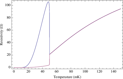

The precise temperature dependence of the DC resistivity is determined by the behavior of and the quasiparticle scattering time . At temperatures near the rounded finite-temperature phase transition, can be identified with the order parameter of the particular finite-temperature phase transition. We expect this classical phase transition to be described by a theory lying on the Ashkin-Teller half-line or equivalently, the moduli space of the orbifold theory. All theories along the line possess a global symmetry and an order parameter for the -broken phase with critical exponent [17] [18]. Since the Kosterlitz-Thouless critical point lies at the boundary point of this half-line, we expect the particular critical theory governing the transition to be largely determined by the degree of rotation symmetry-breaking in the experimental system. Since the in-plane field appears to be a weak symmetry-breaking field, as discussed in the Introduction, we expect the transition to be fairly sharp.
For definiteness below, we take the transition to be in the universality class of the critical four-state Potts model which lies at the boson radius on the orbifold line. In Fig.1 are plotted the resistivities, . The order parameter for this transition , where [19]. (There is not a significant qualitative difference in the plots if the system has the full rotation symmetry so we have suppressed a separate discussion of the KT transition.)
The microscopic parameters in (30) are determined using the resistance measurements performed in [5] as follows. For simplicity, we assume rotationally invariant relations between resistivities and resistances, and , where is some function depending on the sample lengths . In other words, we ignore possible geometrical enhancements that may be present in translating between these two sets of quantities. (See [20] for a discussion of the importance of this distinction in the context of anisotropic transport in half-filled Landau levels [6].) The measured temperature dependences of and at zero in-plane field are fit well by Arrhenius plots, , with and . We continue to use these values in the anisotropic regime, which we identify with the region , when the in-plane field is of sufficient magnitude. The temperature-independent value of over the temperature range implies a quasiparticle scattering lifetime . An estimate of for the maximum value of observed at a tilt angle of and achieved as from above implies with . We stress that the fitting of parameters used to obtain Fig.1 is meant to be as optimistic as possible so as to determine the microscopic parameters of our theory if it is to apply to the experiment.
The height of the peak observed in Fig.1 depends sensitively on the temperature-independent value of . In Fig.2, we plot for three different values of this parameter starting with the value used in Fig.1. As the figure indicates, the peak decreases as this parameter is lowered.
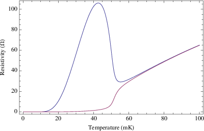
We expect the in-plane magnetic field to act as a small symmetry-breaking field on this finite temperature transition. This will lead to a rounding of the resistivity curves in Fig.1. The order parameter now behaves as
| (32) |
where the is determined by the sign of , and the critical exponents at the four-state Potts point and along the orbifold line. Integral expressions for the scaling functions are known [21]; a precise functional form, however, is not. Scaling dictates that are finite and non-zero, as , and for .
Since we do not have an explicit functional form for , let us simply model the transition using mean field theory in order to obtain a picture for the rounding of the transition. (We do not mean to imply that the crossover function for the transition is in any way similar mean field crossover function. Rather, we only want a picture for how the transition might be rounded.) The mean field critical exponents and . Specification of the free energy, , allows the calculation of via minimization of with respect to . We select the root,
| (33) |
where . It satisfies the scaling requirements detailed in the previous paragraph. Substituting at into our expressions for the resistivities using the same values for the overall scale of the resistivity and behavior of the scattering time as above, we find Fig. 3.
Discussion.
In this paper, we have given an explanation of one of the most striking aspects of the data of Ref. 5: the anisotropy of the longitudinal resistances coexisting with quantized Hall resistance. Our theory further predicts that, while one of the resistances will increase with decreasing temperature at temperatures just below the (rounded) finite-temperature phase transition at which nematic order develops, as observed [5], both longitudinal resistances will, eventually, go to zero at the lowest temperatures, which is yet to be observed. Transport beyond the linear regime, the nature of the massive quasiparticles in the anisotropic phase, and a more complete determination of the values of the parameters in the effective Lagrangian in terms of microscopic variables are interesting open problems.
Acknowledgements.
We thank J. Chalker, J. P. Eisenstein, E. Fradkin, S. Kivelson, H. Liu, J. McGreevy, S. Shenker, S. Simon and J. Xia for helpful discussions, and thank the Aspen Center for Physics for hospitality. M. M. acknowledges the hospitality of the Stanford ITP, the Galileo Galilei ITP and INFN, and Oxford University while this work was in progress. M. M. was supported in part by funds provided by the U. S. Department of Energy (D. O. E.) under cooperative research agreement DE-FG0205ER41360. C.N. was supported in part by the DARPA-QuEST program.References
- [1] M. Mulligan, C. Nayak, and S. Kachru, Phys. Rev. B 82, 085102 (2010).
- [2] S. L. Sondhi, A. Karlhede, S. A. Kivelson, and E. H. Rezayi, Phys. Rev. B 47, 16419 (1993).
- [3] S. E. Barrett, G. Dabbagh, L. N. Pfeiffer, K. W. West, and R. Tycko, Phys. Rev. Lett. 74, 5112 (1995).
- [4] D. A. Abanin, S. A. Parameswaran, S. A. Kivelson, and S. L. Sondhi, Phys. Rev. B 82, 035428 (2010).
- [5] J. Xia, J. P. Eisenstein, L. N. Pfeiffer, and K. W. West, arXiv:1109.3219 (2011).
- [6] M. P. Lilly, K. B. Cooper, J. P. Eisenstein, L. N. Pfeiffer, and K. W. West, Phys. Rev. Lett. 82, 394 (1999a).
- [7] E. Fradkin, S. Kivelson, M. Lawler, J. Eisenstein, and A. Mackenzie, Annu. Rev. Condens. Matter Phys. 1, 153 (2010).
- [8] W. Pan, R. R. Du, H. L. Stormer, D. C. Tsui, L. N. Pfeiffer, K. W. Baldwin, and K. W. West, Phys. Rev. Lett. 83, 820 (1999).
- [9] M. P. Lilly, K. B. Cooper, J. P. Eisenstein, L. N. Pfeiffer, and K. W. West, Phys. Rev. Lett. 83, 824 (1999b).
- [10] J. Xia, V. Cvicek, J. P. Eisenstein, L. N. Pfeiffer, and K. W. West, Phys. Rev. Lett. 105, 176807 (2010).
- [11] S. C. Zhang, T. H. Hansson, and S. Kivelson, Phys. Rev. Lett. 62, 82 (1989).
- [12] One can rewrite this action in terms of so that the Chern-Simons term will have an integer coefficient and the theory can be defined on arbitrary manifolds.
- [13] S. C. Zhang, Int. J. Mod. Phys. B6, 25 (1992).
- [14] W. Kohn, Phys. Rev. 123, 1242 (1961).
- [15] M. P. A. Fisher and D. H. Lee, Phys. Rev. B 39, 2756 (1989).
- [16] K. Musaelian and R. Joynt, J. Phys. 8, 105 (1996).
- [17] The critical exponent of the order parameter field along the orbifold line can be determined using the relation between critical exponents. where is the scaling dimension of the ‘energy’ operator of the CFT. as the boson radius . The twist operator of the CFT has scaling dimension fixed at along the critical line (since it simply acts to change boundary conditions). The critical four-state Potts model and parafermion CFT have and , respectively, while formally diverges at the KT point where the correlation length diverges as as the critical temperature is approached. The exponent characterizing the decay of the order parameter at the critical point with respect to a symmetry-breaking field, , along the critical line.
- [18] Note that a conventional Landau-Ginzburg description of the classical phase transition between a nematically ordered and isotropic state is described by a free energy functional of a symmetric, traceless matrix . Landau-Ginzburg theory predicts a continuous transition when while a first-order transition is expected when because of an allowed cubic term in the free energy. The -invariant critical point we study describes a continuous symmetry-breaking transition with vector order parameter . It is the -invariant director that enters physical quantities like the resistivity and allows the description of a continuous nematic transition in terms of certain response functions.
- [19] F. Y. Wu, Rev. Mod. Phys. 54, 235 (1982).
- [20] S. H. Simon, Phys. Rev. Lett. 83, 4223 (1999).
- [21] S. L. Lukyanov and A. B. Zamolodchikov, Nucl.Phys. B493, 571 (1997).
Appendix.
In this Appendix, we show that, as a result of the violation of the conditions of Kohn’s theorem, the location of the cyclotron pole can vary as is increased. (It is also possible that additional spectral weight shows up at , but we shall not study this possibility in any detail.) We do this by identifying the leading pole in the density-density response with the gap between the lowest and first-excited states in the center-of-mass part of the quantum mechanical many-body wave function. This identification is correct for vanishing in-plane field and we believe it holds for perturbatively small values of as well, where separation of variables into center-of-mass and relative coordinates is well-defined. Of course, this simple example can, at best, give us a few clues about the real system, which is far more complicated. One of these is that the pole moves towards the origin (at least initially) as is increased from zero. This justifies our study of the model (1) with varying .
We begin with the quantum mechanics problem of two mutually interacting three-dimensional electrons in a background magnetic field. This can be easily generalized to an arbitrary number of particles. We take their motion along the plane to be unconstrained but subject to a confining potential along the -direction. The Hamiltonian is
| (34) | |||||
| (35) |
where labels the position of the two particles. (The gauge chosen for the vector potential is consistent with a spatial geometry that is of a finite length along the -directions, and infinite along the -direction. Note, however, we are essentially ignoring the finite length along the -direction in the discussion below so we can think of it as being large compared to the length scale provided by the confining potential along the -direction.)
We consider the component of the magnetic field lying along the -direction to be a perturbation to the system. It is convenient to switch coordinates to the center-of-mass and relative coordinate frame. Choosing
| (36) |
the Hamiltonian becomes
| (37) | |||||
| (38) | |||||
| (39) |
Aside from the confining potentials , the center-of-mass and relative coordinates are decoupled.
At , motion in the -direction decouples from the motion in the plane and we are left with a collection of two-dimensional electrons indexed by their band or energy along the -direction. (Here, we are assuming the pair potential only depends on the separation of the electrons in the plane; the well width is assumed small compared to the magnetic length . This is not the case in the experiments of Refs. 10, 5, so the violations of Kohn’s theorem will be larger than in our simple model.) Given a -eigenfunction, the center-of-mass part of the wave function executes oscillatory motion at the cyclotron frequency . This is the generalization of Kohn’s theorem to the situation where electrons are confined along the direction parallel to the magnetic field. When the spacing between the energy levels of the -eigenfunctions greatly exceeds the cyclotron frequency, it is possible to ignore higher sub-bands when considering low-energy properties of the system. However, this is not the case in the experiments of Refs. 10, 5.
Now consider . There is now a direct mixing between motion in the -direction and motion in the plane. This mixing mediates a coupling at higher orders in between the planar center-of-mass and relative degrees of freedom. Thus, there there is no requirement of a pole at the cyclotron frequency in the density-density correlator. This follows from the fact that the full three-dimensional Galilean symmetry (except for translations) is broken when there is both an in-plane field and a non-zero confining potential along the direction normal to the plane. If either the confining well or in-plane field are removed, there will be a Kohn pole at .
We would like to better understand departures of the pole from the cyclotron frequency in this more general situation with non-zero in-plane field. Namely, we would like to know how the location of the pole varies with . We can obtain some intuition by studying a special case for the form of the confining potential. Take the confining potential to be quadratic, . Then, because
| (40) |
the center-of-mass and relative coordinate motion are still decoupled. This decoupling is not generic; a quartic potential, for example, couples and together. However, we will argue that some conclusions drawn from the quadratic case are general.
We know that at , the Kohn pole corresponds to the splitting between the ground and first excited states of the center-of-mass motion. The relative coordinate is irrelevant both when and for a quadratic electric potential, and so we drop it from our discussion. Thus, the Hamiltonian we study perturbatively in is
| (41) |
where
| (42) | |||||
| (43) | |||||
| (44) |
First, we note that translation invariance along the -direction allows us to replace derivatives with respect to with the momentum along this direction. Next, we shift the coordinate by defining . The Hamiltonian has the form,
| (45) | |||||
| (46) |
where terms proportional to are taken to be a perturbation.
Our goal is to determine the spectral flow as a function of of the ground and first excited energy levels. Dividing out by the irrelevant factor (which determines the degeneracy of the Landau levels in a rectangular sample, but is inconsequential here), the eigenfunctions of the above coupled harmonic oscillator Hamiltonian at take the form:
| (47) | |||||
| (48) |
where , , , denote Hermite polynomials, and the are normalization constants. We assume that .
(For electrons moving in a Ga-As quantum well at , we can estimate and . Given a band mass , where is the free electron mass and transverse magnetic magnetic field of T, we estimate an . has engineering dimension equal to so we take it to be proportional to , where is the well width which is 40 nm for the experiment in [5]. We fix the order of the proportionality constant via the estimate of the Landau level sub-band gap given in Fig. 2 of [10]. We find , where . Thus, . As the filling fraction is lowered, the ratio is increased and so the discussion below becomes less relevant as the two scales are too far apart. Note also that this ratio approaches unity as the proportionality constant between the band and free electron masses is lowered.)
The perturbative shift in the energy of a state to second order in is given by the formula,
| (49) |
where is the unperturbed energy of the state . We are interested in the difference . At zeroth-order, this difference is equal to the cyclotron frequency, . The first-order term on the RHS of (49) vanishes because the perturbation is linear in both and (the ground state is nodeless). Now consider the second-order term. The state (or collection of states since we are ignoring the dependence) mixed with the ground state by the perturbation is , while is the state mixed with . Because the wave functions factorize,
| (50) |
however,
| (51) |
with both energy denominator differences being negative. So while both and are shifted downwards, the ground state is shifted less than the first excited state because of the difference in magnitude of the energy denominators. This implies that the location of the would-be Kohn pole is decreased from the cyclotron frequency. (There is no contradiction with general level repulsion expectations as we are studying a systems with more than two states.) Notice that this result requires mixing between the different -bands and is not present if we take the gap between these energy levels to infinity. Contributions from other excited states only occur at higher orders in perturbation theory. Note also that we dropped a term in the perturbing Hamiltonian quadratic in and so it could, in principle, compete at the same order as the second-order result above. However, this term has no consequence on the energy difference as it shifts both energies by the same amount.
The above analysis implies that the location of the leading pole in a small momentum expansion of the density-density correlator moves towards the origin as an in-plane field is applied. This conclusion was drawn using a certain form of confining potential in the direction transverse to the plane. How general are these results? If we consider a more general form of the confining potential, there will be a coupling between the center-of-mass and relative degrees of freedom. Nevertheless, for small , our results hold generally. In this limit, we can ignore the coupling between the center-of-mass and relative degrees of freedom. The perturbation couples the planar and motion of the center-of-mass at leading order while the coupling between the planar center-of-mass and relative degrees of freedom only occurs at higher order in perturbation theory in . Although the eigenfunctions will take a different functional form and the spacing between these eigenfunctions will no longer be in regular multiples of , the above argument goes through unchanged as long as the gap between the lowest and first-excited eigenfunction is greater than . If is not small, then we cannot ignore the coupling between the center-of-mass and relative degrees of freedom. This can further modify the distribution of spectral weight, but we do not have any simple argument for whether this coupling will move the pole, broaden the pole into a Lorentzian, or change its spectral weight. At any rate, we can say that the coupling between the center-of-mass and relative degrees of freedom will almost certainly cause further deviations from expectations based on Kohn’s theorem. Happily, the effective field theory (1) describes a system where the would-be Kohn pole is different from the bare cyclotron frequency through the variation of ; we pursue its study in the body of the paper.