1Introduction

1 Introduction

The Truncated Conformal Space approach (TCSA) of Yurov and Zamolodchikov [1] is a widely-used method to study the finite-size dependence of perturbed two-dimensional conformal field theories. It is based on truncating the infinite dimensional Hilbert space to a finite-dimensional system on which the Hamiltonian is studied numerically.¹¹ 1 In this paper we study the original form due to Yurov and Zamolodchikov, not the revised version of [2, 3]. It has been known for a long time that the method has various convergence problems which can reduce its effectiveness [4]. The principal problems are a renormalisation of the coupling constant, a renormalisation of the energy scale and differences between ground state contributions in different sectors, all of which depend on the size of the truncated system (we shall always cut off the size of system by taking all states whose unperturbed energy above the ground state is less than or equal to a given number, which we shall call the truncation level). In a previous paper we showed how the renormalisation of the coupling constant in perturbed boundary conformal field theories could be studied using a variant of standard perturbed-conformal field theory methods [12]. In this paper we extend this study to the second effect, and show how the leading energy scale renormalisation is an overall multiplicative renormalisation which can be considered equivalent to a renormalisation of the size of the system. We find ‘physical’ arguments based on the operator product expansions and also more rigorous arguments based on an analysis of the eigenvalues of the perturbed Hamiltonian and show that these give identical results. We test our results using two integrable conformal field theories, the tri-critical Ising model and the Yang-Lee model, as in both cases the finite-size spectrum has been found using TBA methods and this provides an accurate quantitative check of the proposed results.

In the next section we briefly review the case of the tri-critical model to illustrate the renormalisation issues to be solved and to find numerical estimates for the coupling renormalisation and energy rescaling. We then show that these have scaling forms and find numerical estimates for the associated exponents.

In the third section we show how these can be derived, to one loop order, from considerations of the renormalisation of the perturbed action and in the fourth section show how these can be proven, to leading order, for all energy levels, from analysis of the eigenvalues of the perturbed Hamiltonian. In the subsequent two sections we check these predictions against the numerical data in the tri-critical Ising model and the Yang-Lee model

In section 8 we consider the case of an irrelevant (non-renormalisable) perturbation and in section 9 we consider the flows beyond the fixed points and speculate on the exponents that have been found numerically. Finally in section 10 we present our conclusions.

2 The TCSA approach and its errors

2.1 The TCSA approach

We start with a CFT defined on a strip $0\leq y\leq L$ of width $L$ in the upper half plane with coordinate $z=x+iy$ . We take the strip to have conformally invariant boundary conditions so that the system is conformally invariant, the Hilbert space carries an action of the Virasoro algebra and decomposes into a direct sum of representations of the Virasoro algebra. The representations occurring depend on the boundary conditions on the strip.

The unperturbed CFT Hamiltonian generating translations along the strip is

H=\int_{0}^{L}T_{xx}\;\frac{{\mathrm{d}}y}{2\pi}\;.

(2.1)

We will map the strip to the upper half plane with coordinate $w=\exp(\pi z/L)$ in terms of which the CFT Hamiltonian is

H=\frac{\pi}{L}\left(L_{0}-\frac{c}{24}\right)\;,

(2.2)

where $L_{0}$ is the zero mode of the Virasoro algebra.

We are interested in perturbations by one or more boundary fields $\phi_{i}(x)$ living on the bottom edge of the strip, $y=0$ . We take these to be quasi-primary fields of conformal dimension $h_{i}$ . If the coupling to these fields are $\mu_{i}$ then the perturbation is given by an addition to the action

\delta S=\int\sum_{i}\mu_{i}\phi_{i}(x)\,{\mathrm{d}}x\;.

(2.3)

When mapped to the upper half plane this gives the perturbed Hamiltonian as

H=\frac{\pi}{L}\left[\;\left(L_{0}-\frac{c}{24}\right)\;+\;\sum_{i}\mu_{i}\left(\frac{L}{\pi}\right)^{y_{i}}\,\phi_{i}(1)\right]\;,

(2.4)

where $y_{i}=1-h_{i}$ . Note that (2.4) is only correct if the fields $\phi_{i}$ are primary; there are corrections if they are quasi-primary but not primary. We will normally consider the dimensionless operator

\mathcal{H}=\left(\frac{L}{\pi}\right)H=\left(L_{0}-\frac{c}{24}\right)\;+\;\sum_{i}\frac{\lambda_{i}}{\pi^{y_{i}}}\,\phi_{i}(1)\;,

(2.5)

where $\lambda_{i}=\mu_{i}L^{y}$ are dimensionless coupling constants.

The TCSA approach is to restrict this Hamiltonian to a finite dimensional space of excitation level $n$ or lower. If we take the projector onto this space to be $P_{n}$ then the TCSA Hamiltonians are

\mathcal{H}_{n}=\left(L_{0}-\frac{c}{24}\right)\;+\;\sum_{i}\frac{\lambda_{i}}{\pi^{y_{i}}}\,P_{n}\phi_{i}(1)P_{n}\;.

(2.6)

These Hamiltonians can be diagonalised numerically and their eigenvalues and eigenstates form the TCSA approximations to the perturbed system. Any quantity that can be considered in the perturbed system can also be considered in the TCSA system; the only question is how good the approximation is, and whether the dependence on the truncation level is either small or can be estimated efficiently. In the next section we present the two leading truncation effects — the renormalisation of the coupling constant and the rescaling of the energy levels — in the case of the tri-critical Ising model.

2.2 The tri-critical Ising model numerical results

We take as our example model example the boundary tri-critical Ising model on a strip. We shall review the boundary conditions and their flows in section 5; for the moment it is sufficient to know that, amongst others, there are conformal boundary conditions labelled $(11)$ , $(21)$ and $(12)$ , and the $(12)$ boundary condition can be perturbed by a field of weight $3/5$ with the following flows:

(11)\longleftarrow(12)\longrightarrow(12)\;.

(2.7)

The spectrum of the Hamiltonian on a strip with an unperturbed $(11)$ and a perturbed $(12)$ boundary condition has also been analysed from the TBA approach by Feverati and collaborators in [7]. Using the results in [21] and [22, 23], we can relate the TBA and conformal perturbation theory parameters and so we can compare the TCSA spectrum to the exact perturbed conformal field theory spectrum for this system.

The most immediate difference is that there is an overall shift in the energy levels. For finite perturbations for which there are no divergences in the perturbation expansion this corresponds to a measurable free energy per unit length. In this case the perturbation theory is divergent and the overall shift in the energies is not meaningful: in TCSA it depends on the truncation level and does not converge to a finite value. As a consequence, in figure 1 we just show the difference between the ground state and the excited states - the energy gaps: in figure 1(a) we give the gaps as calculated using the TBA method, and in figure 1(b) the TCSA gaps.

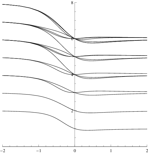
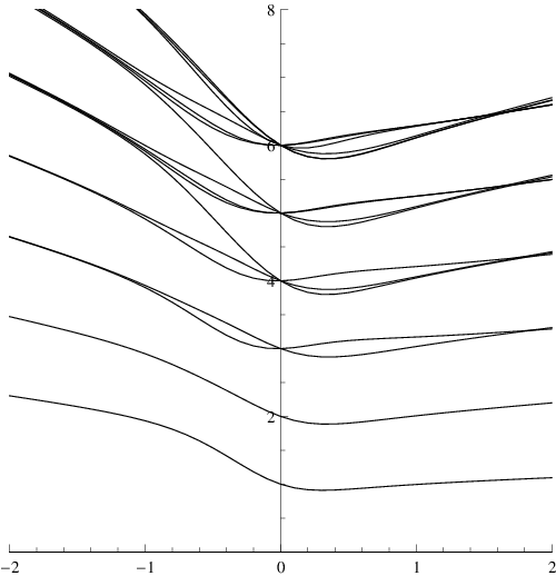
On inspection of figure 1, one can also discern the two other effects. In the TCSA plot, there is an apparent convergence of many levels at or near $\lambda=2$ . This corresponds to a fixed point of the flow where the $(12)$ boundary condition has reached its $(21)$ fixed point. This is only reached at $\lambda=\infty$ in the TBA flow. The two couplings are related by a non-trivial renormalisation. Less obvious but still measurable is the overall rescaling of the energy levels. At $\lambda=-2$ the TCSA spectrum has almost regrouped into equally-spaced levels but the spacing is approximately 15% larger than the (correct) spacing in the TBA spectrum. This effect grows markedly with increasing $|\lambda|$ .

We can find numerical estimates for the renormalisation (of the coupling constant) and rescaling (of the energy scale) by comparing the TCSA and TBA data. Firstly we consider only the energy gaps to remove the unphysical ground state energy contributions in the TCSA scheme. Next, since both the overall scale and the value of the coupling are different, we consider the ratio of two gaps to find a quantity which is independent of the energy rescaling and use this to determine the effective coupling constant. We can then use this in turn to find the energy rescaling.

If we denote the coupling constant in TCSA by $\lambda_{n}$ and that in the TBA by $\lambda_{\infty}$ , and the $n^{th}$ energy gaps by $\Delta^{n}_{n}$ and $\Delta^{n}_{\infty}$ respectively, then we can calculate

f_{\infty}(\lambda_{\infty})=\frac{\Delta^{2}_{\infty}}{\Delta^{1}_{\infty}}\;,\;\;f_{n}(\lambda_{n})=\frac{\Delta^{2}_{n}}{\Delta^{1}_{n}}\;,

(2.8)

We can then find the effective (TBA) coupling corresponding to a given TCSA coupling from the function $g_{n}$ defined by

\lambda_{\infty}=f_{\infty}^{-1}(f_{n}(\lambda_{n}))=\lambda_{n}g_{n}(\lambda_{n})\;,

(2.9)

and the energy rescaling $r_{n}(\lambda_{n})$ can then be found from

r_{n}(\lambda_{n})=\frac{\Delta^{1}_{n}(\lambda_{n})}{\Delta^{1}_{\infty}(\lambda_{\infty})}\;.

(2.10)

In figure 2 we plot these functions for the flows starting from the $(12)$ boundary condition for three different truncation levels. It is the aim of this paper to show how these two effects can predicted from physical and mathematical arguments.

3 Physical Arguments

3.1 The TCSA renormalisation group

In [12], we presented an argument deriving the leading term in the coupling constant renormalisation based on standard considerations of the partition function and the operator product expansion of the perturbing field. We repeat this argument here in a little more generality, both as a derivation of the coupling constant renormalisation which we shall check in the next section, but also to show that this does not in fact give the leading term to the energy rescaling, as might have been thought was the case.

We consider a strip geometry of width $L$ with complex coordinate $z=x+iy$ with $0\leq y\leq L$ . We take a general boundary perturbation of the form

\sum_{i}\mu_{i}\phi_{i}(x)\;,

(3.1)

where $\mu_{i}$ are the couplings to the boundary fields $\phi_{i}$ which have conformal weights $h_{i}$ . We define $y_{i}=1-h_{i}$ .

We consider a truncation to level $n$ which we can treat using a projection operator $P_{n}$ onto states of excitation level $n$ or below. We can use the projection operator to restrict the perturbation to the truncated Hilbert space so that the TCSA approximation to the perturbation 3.1 is then given by

\sum_{i}\mu_{i}(P_{n}\phi_{i}P_{n})\;.

(3.2)

The effect of the perturbation is to introduce the following operator

\mathcal{P}\exp\left(-\int_{x=-\infty}^{\infty}\sum_{i}\mu_{i}(P_{n}\phi_{i}(x)P_{n})\,{\mathrm{d}}x\right)\;,

(3.3)

into all expectation values, where $\mathcal{P}$ is path ordering. Mapping the strip to the upper half plane by $w=\exp(\pi z/L)$ , this operator becomes

\mathcal{P}\exp\left(-\int_{x=0}^{\infty}\sum_{i}\lambda_{i}(P_{n}\phi_{i}(x)P_{n})\frac{{\mathrm{d}}x}{(x\pi)^{y_{i}}}\right)\;,

(3.4)

where $\lambda_{i}=\mu_{i}L^{y_{i}}$ is the dimensionless coupling constant.

Expanding this exponential out to second order we get

	$\displaystyle 1$	$\displaystyle-$	$\displaystyle\sum_{i}\lambda_{i}\int_{x=0}^{\infty}P_{n}\phi_{i}(x)P_{n}\frac{{\mathrm{d}}x}{(x\pi)^{y_{i}}}$		(3.5)
		$\displaystyle+$	$\displaystyle\sum_{jk}\lambda_{j}\lambda_{k}\int_{x=0}^{\infty}\int_{x^{\prime}=0}^{x}P_{n}\phi_{j}(x)P_{n}\phi_{k}(x^{\prime})P_{n}\frac{{\mathrm{d}}x}{(x\pi)^{y_{j}}}\frac{{\mathrm{d}}x^{\prime}}{(x^{\prime}\pi)^{y_{k}}}\;+\;O(\lambda^{3})\;.$		(3.5)

We define the TCSA renormalisation group by the requirement that the partition function is unchanged when the truncation level is increased. This introduces a level dependence into the coupling constants, which we now denote by $\lambda_{i}(n)$ .

Due to translation invariance, we do not need to compare the whole expression in equation 3.5, instead we can just compare the integrand with respect to $x$ , at $x=1$ , which is

\sum_{i}\frac{\lambda_{i}(n)}{\pi^{y_{i}}}P_{n}\phi_{i}(1)P_{n}-\sum_{jk}\frac{\lambda_{j}(n)}{\pi^{y_{j}}}\frac{\lambda_{k}(n)}{\pi^{y_{k}}}\int_{x^{\prime}=0}^{1}P_{n}\phi_{j}(1)P_{n}\phi_{k}(x^{\prime})P_{n}\frac{{\mathrm{d}}x^{\prime}}{(x^{\prime})^{y_{k}}}+O(\lambda^{3})\;.

We can further simplify matters by assuming that the Hilbert space contains a vacuum state ${{|{0}\rangle}}$ and a state ${|{\phi_{i}}\rangle}$ corresponding to the field which satisfy

{\langle{\phi_{i}}|}\phi_{j}(1){{|{0}\rangle}}=\delta_{ij}\;,\;\;{\langle{\phi_{i}}|}\phi_{j}(1)\phi_{k}(x){{|{0}\rangle}}=(1-x)^{x_{i}-x_{j}-x_{k}}C_{ijk}\;.

(3.6)

Sandwiching equation 3.1 between the states ${\langle{\phi_{i}}|}$ and ${{|{0}\rangle}}$ , we get

\lambda_{i}(n)-\sum_{jk}\lambda_{j}(n)\lambda_{k}(n)\int_{x=0}^{1}{\langle{\phi_{i}}|}\phi_{j}(1)\,P_{n}\,\phi_{k}(x){{|{0}\rangle}}(\pi x)^{y_{i}-y_{j}-y_{l}}{\mathrm{d}}x+O(\lambda^{3})\;.

(3.7)

This must be invariant under changes in $n$ so that two second order in $\lambda$ . Using the fact that ${\langle{\phi_{k}}|}\phi_{i}(1)(P_{n+1}-P_{n})\phi_{j}(x){{|{0}\rangle}}$ is the coefficient of $x^{n+1}$ in the expansion of $(1-x)^{h_{i}-h_{j}-h_{k}}$ and is equal to

\frac{\Gamma(h_{j}+h_{k}-h_{i}+n+1)}{\Gamma(h_{j}+h_{k}-h_{i})\Gamma(n+2)}=\frac{n^{y_{i}-y_{j}-y_{k}}}{\Gamma(h_{j}+h_{k}-h_{i})}(1+O(1/n))\;,

(3.8)

we find the TCSA renormalisation group equations

n\frac{{\mathrm{d}}\lambda_{i}}{{\mathrm{d}}n}\simeq n(\lambda_{i}(n+1)-\lambda_{i}(n))=\sum_{jk}\lambda_{j}\lambda_{k}(n\pi)^{y_{i}-y_{j}-y_{k}}\frac{C_{ijk}}{\Gamma(h_{j}+h_{k}-h_{i})}+O(\lambda^{3})\;.

(3.9)

3.2 The coupling constant renormalisation

In the case of the perturbation by a single field with self-coupling $C$ , the TCSA renormalisation group equation (3.9) becomes

n\frac{{\mathrm{d}}\lambda}{{\mathrm{d}}n}=\frac{C}{\Gamma(h)(n\pi)^{y}}\lambda^{2}+O(\lambda^{3})\;,

(3.10)

with solution

\lambda(\infty)=\frac{\lambda(n)}{\displaystyle 1\;\;-\;\;\frac{C}{y\Gamma(h)(n\pi)^{y}}\,\lambda(n)}\;.

(3.11)

There are two predictions from this calculation - firstly the general prediction that the coupling renormalisation has a particular scaling form, namely that the function $g_{n}$ in equation 2.9 has the form

g_{n}(x)=g(xn^{-y})\;,

(3.12)

and secondly a particular prediction for the 1-loop behaviour,

g(x)=\left(1-\frac{Cx}{y\Gamma(h)\pi^{-y}}\right)^{-1}+O(x^{2},n^{-2y})

(3.13)

We test these predictions for the tri-critical Ising model in section 5.1. We will find that the functions $\log(g_{n}(-xn^{y}))$ are indeed almost identical for various values of $n$ and in good agreement with the prediction, confirming both the prediction of the scaling form and the approximate numerical expression for this scaling function.

3.3 The energy rescaling

We can try to apply the same arguments to derive the energy rescaling, assuming that this too comes from the operator product of the perturbing fields giving a contribution to the bare action (corresponding to the kinetic term in a standard Lagrangian theory). The Bare Hamiltonian is $(\pi/L)(L_{0}-c/24)$ . The important part is the term $L_{0}$ which is a mode of the energy-momentum tensor $T(z)$ . This field appears in the operator product of the boundary perturbing field as

	$\displaystyle\phi(z)\;\phi(w)$	$\displaystyle\sim$	$\displaystyle\frac{1}{(z-w)^{2h}}+\frac{C}{(z-w)^{h}}\phi(w)+\frac{h/c}{(z-w)^{2h-2}}T(w)+\ldots\;,\;\;$		(3.14)
	$\displaystyle T(z)\;\phi(w)$	$\displaystyle\sim$	$\displaystyle\frac{2h}{(z-w)^{2}}\phi(w)+\frac{1}{z-w}\phi^{\prime}(w)+\ldots\;,\;\;$		(3.15)

where we have also included the OPE of $T$ with the perturbing field.

If we denote the coupling to the perturbing field by $\lambda$ and to the energy momentum tensor on the boundary by $\lambda_{T}$ we then have $h_{T}=2$ , $y_{T}=-1$ and we find the TCSA renormalisation group equations become

	$\displaystyle n\frac{{\mathrm{d}}\lambda}{{\mathrm{d}}n}$	$\displaystyle=$	$\displaystyle\frac{C}{(n\pi)^{y}\Gamma(h)}\lambda^{2}+(4hn\pi)\lambda\lambda_{T}+\ldots\;,$		(3.16)
	$\displaystyle n\frac{{\mathrm{d}}\lambda_{T}}{{\mathrm{d}}n}$	$\displaystyle=$	$\displaystyle\frac{2h/c}{(n\pi)^{1+2y}\Gamma(-2y)}\lambda^{2}+\ldots\;.$		(3.17)

To find the leading dependence on the induced coupling $\lambda_{T}$ we can take $\lambda$ to be constant and using $\lambda_{T}(\infty)=0$ , find

	$\displaystyle\lambda_{T}(n)$	$\displaystyle=$	$\displaystyle-\int_{n}^{\infty}\frac{{\mathrm{d}}\lambda_{T}}{{\mathrm{d}}n}{\mathrm{d}}n$		(3.18)
		$\displaystyle=$	$\displaystyle-\frac{2h/c}{\Gamma(-2y)(1+2y)}\frac{\lambda^{2}}{(n\pi)^{2y+1}}+O(\lambda^{3})\;.$		(3.18)

The addition of the term

\int\mu_{T}T(x){\mathrm{d}}x\;,

(3.19)

to the action will give the following term to the Hamiltonian (after mapping from the strip to the upper half plane)

\delta H=\mu_{T}T(1)=\frac{\pi}{L}\left(-\frac{2h/c}{\Gamma(-2y)(1+2y)}\frac{\lambda^{2}}{(n\pi)^{2y}}\frac{1}{n}\Big(L_{0}-c/24\Big)+\hbox{other modes}\right)\;,

(3.20)

so that the Hamiltonian becomes

H+\delta H=\frac{\pi}{L}\left(1-\frac{2h/c}{\Gamma(-2y)(1+2y)}\frac{\lambda^{2}}{(n\pi)^{2y}}\frac{1}{n}\right)\Big(L_{0}-c/24\Big)+\ldots\;,

(3.21)

This gives the rescaling function as

r_{n}(\lambda)=1-\frac{2h/c}{\Gamma(-2y)(1+2y)}\frac{\lambda^{2}}{(n\pi)^{2y}}\frac{1}{n}+\ldots\;.

(3.22)

Unfortunately, this has the wrong $n$ -dependence - it is one order of $n$ too small. If we plot $\log(r_{n}(\lambda)-1)$ against $\log(n)$ for fixed $\lambda$ for the functions shown in figure 1(b), in the tri-critical Ising model, we find that the prediction for the leading exponent

\log(r_{n}(\lambda)-1)=\alpha\log(n)+\ldots\;,

(3.23)

is approximately $\alpha=-0.85$ , which is close to $-2y=-0.8$ and far from $-1-2y=-1.8$ . As a consequence, we deduce that the coupling of the perturbing fields to the energy-momentum tensor is not the leading source of the correction to the energy rescaling function.

Instead we look to the constant ground-state energy contribution coming from the coupling to the identity operator. As we show in the next section, this is actually not a constant because of the presence of the projector $P_{n}$ and this can also give a correction proportional to the bare Hamiltonian.

3.4 Corrections from the identity operator

In perturbation theory where the perturbing field has a weight greater than 1/2 one normally ignores the ground state energy as it is a divergent unphysical quantity. In this case the TCSA cutoff makes the contribution finite, and further more, the presence of the projector $P_{n}$ means it is not constant.

We are interested in the correction to the coupling to the identity operator which arises when the expression 3.1 acts on a state of excitation level $E$ . If we denote this state by ${|{E}\rangle}$ and the coupling to the identity by $\lambda_{1}(E,n)$ , then we are interested in the expression

\displaystyle\frac{\lambda_{1}(E,n)}{\pi}-\frac{\lambda(n)^{2}}{\pi^{2y}}\int_{x^{\prime}=0}^{1}{\langle{E}|}\phi(1)P_{n}\phi(x^{\prime}){|{E}\rangle}\frac{{\mathrm{d}}x^{\prime}}{(x^{\prime})^{y}}

(3.24)

Requiring that this be invariant as we change the truncation level $n$ , we get

	$\displaystyle\frac{{\mathrm{d}}\lambda_{1}(E,n)}{{\mathrm{d}}n}$	$\displaystyle\simeq$	$\displaystyle(\lambda_{1}(E,n+1)-\lambda_{1}(E,n))$		(3.25)
		$\displaystyle=$	$\displaystyle\frac{\lambda(n)^{2}}{\pi^{2y}}\int_{x=0}^{1}{\langle{E}\|}\phi(1)(P_{n+1}-P_{n})\phi(x){\|{E}\rangle}\frac{{\mathrm{d}}x}{(x)^{y}}\;,$		(3.25)

where we only take the contribution to the OPE on the right hand side that comes from the identity channel. The projector $(P_{n+1}-P_{n})$ picks out the state at level $n+1$ in the action of the field $\phi(x)$ on the state ${|{E}\rangle}$ . The action of the field $\phi(x)$ on the state ${|{E}\rangle}$ has a mode expansion

\phi(x){|{E}\rangle}=\sum\phi_{m}x^{m-h}{|{E}\rangle}\;,

(3.26)

so that the term at excitation level $n$ is just the coefficient of $x^{n+1-E}$ . From the operator product expansion (3.14), the coefficient of $x^{n+1-E}$ in ${\langle{E}|}\phi(1)\phi(x){|{E}\rangle}$ is

\frac{\Gamma(n+1-E+2h)}{\Gamma(n+2-E)\Gamma(2h)}\;,

(3.27)

This means that the leading contribution to the RG equation (3.25 for the coupling $\lambda_{1}$ is

$\displaystyle\frac{{\mathrm{d}}\lambda_{1}(E,n)}{{\mathrm{d}}n}$	$\displaystyle\simeq$	$\displaystyle\frac{\lambda(n)^{2}}{\pi^{2y}}\int_{x=0}^{1}\frac{\Gamma(n+1-E+2h)}{\Gamma(n+2-E)\Gamma(2h)}x^{n+1-E}\frac{{\mathrm{d}}x}{(x)^{y}}$	(3.28)
	$\displaystyle\simeq$	$\displaystyle\frac{\lambda^{2}}{\pi^{2y}}\frac{(n-E)^{2h-2}}{\Gamma(2h)}+\ldots$
	$\displaystyle\simeq$	$\displaystyle\frac{\lambda^{2}}{(n\pi)^{2y}}\frac{1}{\Gamma(2h)}\left(1\;+\;2y\frac{E}{n}+\ldots\right)$

The first term is the constant contribution which we shall now ignore; the second is the excitation-level dependant term which we are interested in. We can integrate equation (3.28) using the boundary condition $\lambda_{1}(E,\infty)=0$ , to find

	$\displaystyle\lambda_{1}(E,n)\big\|_{E}$	$\displaystyle=$	$\displaystyle-\int_{n}^{\infty}\frac{\lambda^{2}}{\pi^{2y}}\frac{1}{\Gamma(2h)}2yEn^{-2y-1}{\mathrm{d}}n$		(3.29)
		$\displaystyle=$	$\displaystyle\frac{\lambda^{2}}{(n\pi)^{2y}}\frac{1}{\Gamma(2h)}E\;.$		(3.29)

We can now replace the excitation level $E$ by the operator $(L_{0}-c/24)$ , as $E$ is approximately the eigenvalue of $(L_{0}-c/24)$ , and we finally find we have generated a term proportional to the bare Hamiltonian. We have two equivalent ways of understanding this term which lead to the same expression for the energy rescaling $r_{n}(\lambda)$

Firstly, we can see that this coupling will lead directly to a change in the Hamiltonian; the new Hamiltonian is

\frac{\pi}{L}\left[(1+\frac{\lambda^{2}}{(n\pi)^{2y}}\frac{1}{\Gamma(2h)})(L_{0}-c/24)+\frac{\lambda}{\pi^{y}}\phi(1)\right]\;,

(3.30)

giving the energy rescaling function as

r_{n}(\lambda)=1+\frac{\lambda^{2}}{(n\pi)^{2y}}\frac{1}{\Gamma(2h)}+\ldots\;,\;\;r(x)=1+\frac{x^{2}}{\pi^{2y}}\frac{1}{\Gamma(2h)}+\ldots\;.

(3.31)

This has the correct $n$ dependence (in agreement with the numerical data) and is also a very good fit to the actual rescaling function as we see in section 5.2.

An alternative viewpoint of the energy rescaling function is that it represent an effective change in the geometry of the system. Coordinate transformations are implemented in CFT by changes to the action (see e.g. [13]). The coordinate change $x^{\mu}\to\alpha^{\mu}+\alpha^{\mu}$ corresponds to the change in the action

\delta S=-\frac{1}{2\pi}\int T_{\mu\nu}\partial^{\mu}\alpha^{\nu}\;{\mathrm{d}}^{2}x\;.

(3.32)

The energy-dependant correction to the identity operator we have just calculated can also be put in this form. On the upper-half-plane, with complex coordinate $w=r\exp(i\theta)$ , the correction is

\delta S=-\frac{1}{\pi}\int\lambda_{1}(E,n)\frac{{\mathrm{d}}r}{r}=-\frac{\lambda^{2}}{(n\pi)^{2y}\Gamma(2h)}\int L_{0}\frac{{\mathrm{d}}r}{r}\;.

(3.33)

Firstly, we note that on the upper half plane

L_{0}=\frac{\pi}{L}\int_{\theta=0}^{\pi}(w^{2}T(w)+\bar{w}^{2}\bar{T}(\bar{w}))\frac{{\mathrm{d}}\theta}{2\pi}\;.

(3.34)

Combining equations (3.33) and (3.34) and transforming to the strip with coordinate $z=x+iy$ , the correction to the action becomes

\delta S=-\frac{\lambda^{2}}{(n\pi)^{2y}\Gamma(2h)}\int T_{xx}\frac{{\mathrm{d}}x\,{\mathrm{d}}y}{2\pi}\;,

(3.35)

which in turn corresponds to the change in coordinates

\pmatrix{x\cr y}\to\pmatrix{x\left(1+\frac{\lambda^{2}}{(n\pi)^{2y}\Gamma(2h)}\right)\cr y}=\pmatrix{r_{n}(\lambda)x\cr y}\;.

(3.36)

If we consider the theory on a strip of length $R$ then this change in coordinates is an effective increase in the length by a factor $r_{n}(\lambda)$ . To the order in $\lambda$ to which we are working, this is equivalent to a reduction in the strip width by the same factor and consequently a rescaling of the eigenvalues of the Hamiltonian by the same factor, $r_{n}(\lambda)$ , exactly in accordance with equation (3.31).

4 Mathematical Arguments

It is also possible to derive the coupling constant renormalisation and energy rescaling by examining the lowest three eigenvalues of the perturbed, truncated Hamiltonian directly. This gives exact expressions in terms of integrated four-point functions of the conformal field theory. We can then find the large- $n$ behaviour of these eigenvalues by a saddle-point approximation. It turns out that these are given in terms of the crossed four-point functions and the leading large- $n$ behaviour is given by the leading terms in the crossed four-point functions, which are in turn given by the operator product expansion coefficients. In this way we see that the “physical” arguments of the previous section are indeed correct. Furthermore, we can show that the corrections we have found are the leading order corrections for all the eigenvalues of the perturbed Hamiltonian, not just the lowest three.

We start from the expression (2.6) for the dimensionless TCSA Hamiltonian:

\mathcal{H}_{n}=(L_{0}-\frac{c}{24})+{\tilde{\lambda}}P_{n}\phi(1)P_{n}\;.

(4.1)

We have introduced $\tilde{\lambda}=\lambda\pi^{-y}$ for notational convenience.

For simplicity we consider a case where the Hilbert space is a single highest weight representation of the Virasoro algebra with conformal weight $H$ , and that the two lowest level states are

{|{\psi}\rangle}\;,\;\;L_{-1}{|{\psi}\rangle}\;.

(4.2)

We will assume that the the energy-rescaling and coupling constant renormalisation take the forms (3.12) and

g(x)=1+b\pi^{-y}x+O(x^{2},n^{-2y})\;,\;\;r(x)=1+a\pi^{-2y}x^{2}+O(x^{3},n^{-3y})\;.

(4.3)

We also assume that the first energy gap takes the exact form

\Delta_{1}(\lambda)=E_{1}(\lambda)-E_{0}(\lambda)=1+\alpha{\tilde{\lambda}}+\beta{\tilde{\lambda}}^{2}+O(\lambda^{3})\;,

(4.4)

so that the TCSA approximation at truncation level $n$ is given by

	$\displaystyle\Delta_{1}^{n}(\lambda)$	$\displaystyle=$	$\displaystyle r(\lambda n^{-y})\Delta_{1}(\lambda g(\lambda n^{-y}))$		(4.5)
		$\displaystyle=$	$\displaystyle 1+\alpha{\tilde{\lambda}}+{\tilde{\lambda}}^{2}(\beta+an^{-2y}+b\alpha n^{-y})+O(\lambda^{3},n^{-3y})\;.$		(4.5)

This means that we can find the coefficients $a$ and $b$ appearing in the rescaling and renormalisation functions (4.3) from the $n$ dependence in the second order term in the first energy gap. From the physical arguments of the previous section, we expect

a=\frac{1}{\Gamma(2h)}\;,\;\;b=\frac{C}{y\Gamma(h)}\;.

(4.6)

By standard perturbation theory, we find the following expressions for the ground state and first excited state energies, to second order:

$\displaystyle E_{0}$	$\displaystyle=$	$\displaystyle H+{\tilde{\lambda}}C^{\prime}-({\tilde{\lambda}}C^{\prime})^{2}\int_{0}^{1}(F^{0}-\frac{1}{z^{h}})\frac{{\mathrm{d}}z}{z^{y}}\;,\;\;$
$\displaystyle E_{1}$	$\displaystyle=$	$\displaystyle(H+1)+{\tilde{\lambda}}C^{\prime}\left(1+\frac{(h-1)h}{2H}\right)$	(4.7)
		$\displaystyle+({\tilde{\lambda}}C^{\prime})^{2}\left[\frac{h^{2}}{2H}-\int_{0}^{1}\frac{{\mathrm{d}}z}{z^{y}}\left(F^{1}-\frac{h^{2}/(2H)}{z^{2-y}}-\frac{(2H+h(h-1))^{2}}{(2H)^{2}z^{1-y}}\right)\right]\;.$	(4.7)

Here $C^{\prime}$ is the boundary coupling constant in the operator product expansion

\phi(x){|{\psi}\rangle}=\frac{C^{\prime}}{x^{h}}{|{\psi}\rangle}+\ldots\;,

(4.8)

and the function $F^{0}$ is the four point chiral block

F^{0}(z)=\raisebox{-7.11317pt}{\mbox{ $\begin{picture}(3901.0,-2683.0){\put(4800.0,-1860.0){\line{ 0}{-1}{600.0}}}{\put(5700.0,-1860.0){\line{ 0}{-1}{600.0}}}{\put(4200.0,-2460.0){\line{ 1}{ 0}{2100.0}}}\put(4150.0,-2460.0){\pic@makebox@{\makebox}{}(0.0,0.0)[rc]{$\psi$}}\put(4800.0,-1800.0){\pic@makebox@{\makebox}{}(0.0,0.0)[cb]{$\phi$}}\put(4800.0,-2560.0){\pic@makebox@{\makebox}{}(0.0,0.0)[ct]{$1$}}\put(5250.0,-2380.0){\pic@makebox@{\makebox}{}(0.0,0.0)[cb]{$\psi$}}\put(5700.0,-1800.0){\pic@makebox@{\makebox}{}(0.0,0.0)[cb]{$\phi$}}\put(5700.0,-2560.0){\pic@makebox@{\makebox}{}(0.0,0.0)[ct]{$z$}}\put(6400.0,-2460.0){\pic@makebox@{\makebox}{}(0.0,0.0)[lc]{$\psi$}}\end{picture}\;\;$}}=z^{-h}(1+\ldots)\;,

(4.9)

that appears in the boundary two-point function on the strip. Since we have chosen boundary conditions for which the Hilbert space of the model on the strip has only a single representation with highest weight ${|{\psi}\rangle}$ , the boundary two point function is given as the product of the structure constants and the single chiral block with the representation $\psi$ in the intermediate channel:

\langle\phi(1)\phi(z)\rangle_{\mathrm{strip}}={\langle{\psi}|}\phi(1)\phi(z){|{\psi}\rangle}=(C^{\prime})^{2}F^{0}(z)\;.

(4.10)

$F^{1}$ is the function that appears in the two point function of the field $\phi(z)$ in the first excited state,

			$\displaystyle\frac{{\langle{\psi}\|}L_{1}\phi(1)\phi(z)L_{-1}{\|{\psi}\rangle}}{{\langle{\psi}\|}L_{1}L_{-1}{\|{\psi}\rangle}}=(C^{\prime})^{2}F^{1}(z)\;,\;\;$
	$\displaystyle F^{1}(z)$	$\displaystyle=$	$\displaystyle\frac{1}{2H}\left\{\left[z(z-1)\frac{{\mathrm{d}}}{{\mathrm{d}}z}+2zh-1\right]\left[(z-1)\frac{{\mathrm{d}}}{{\mathrm{d}}z}+2h\right]+2H\right\}F^{0}\;.$		(4.11)

If $h$ , the conformal dimension of the perturbing field, is greater than or equal to 1/2 then the integrals in the expressions (4.7) diverge, but their difference, the energy gap $\Delta_{1}$ , is finite. We can read off the coefficients $\alpha$ and $\beta$ that appear in (4.4) as

	$\displaystyle\alpha$	$\displaystyle=$	$\displaystyle\frac{h(h-1)}{2H}C^{\prime}\;,\;\;$		(4.12)
	$\displaystyle\beta$	$\displaystyle=$	$\displaystyle(C^{\prime})^{2}\left\{\frac{h^{2}}{2H}-\int_{0}^{1}\frac{dz}{z^{y}}\left[\left(F^{1}-\frac{h^{2}/(2H)}{z^{2-y}}-\frac{(2H+h(h-1))^{2}}{(2H)^{2}z^{1-y}}\right)-\left(F^{0}-\frac{1}{z^{h}}\right)\right]\right\}$

These are the exact coefficients in the perturbative expansions of the energy gap; we are interested in the $n$ -dependence in the TCSA approximation (4.5). The $n$ -dependence comes from replacing the functions $F^{0}$ and $F^{1}$ in () by the TCSA truncations. We see that $\alpha$ is independent of $n$ but $\beta$ does depend on $n$ ; we shall denote the TCSA truncation by $\beta(n)$ and we expect from (4.5) that

\beta(n)=\beta+an^{-2y}+b\alpha n^{-y}+O(n^{-3y})\;.

(4.14)

As before, in section 3.4, the TCSA truncations of the functions $F^{0}$ and $F^{1}$ come from restricting their Taylor expansions to include only modes up to power $z^{n-h}$ . It is easier to analyse the change in the functions as the TCSA level is increased than to find the $n$ -dependence directly, so we consider the change in $\beta$ given by the taking just the coefficient of $z^{n+y}$ in the integrand of ()

\displaystyle\frac{{\mathrm{d}}\beta}{{\mathrm{d}}n}

\displaystyle\simeq

\displaystyle\beta(n+1)-\beta(n)=\frac{(C^{\prime})^{2}}{n}\oint\frac{{\mathrm{d}}z}{2\pi iz^{n+1}}\left[z^{h}(F^{0}-F^{1})\right]\;.

(4.15)

The contour in (4.15) is a small circle around the origin. The function $z^{h}(F^{1}-F^{0})$ is single valued around the origin but has a cut from $z=1$ to $z=\infty$ , and can be expanded in increasing powers of $(1-z)^{-1}$ . We use the result that

\oint\frac{{\mathrm{d}}z}{2\pi iz^{n+1}}(1-z)^{-\alpha}=\frac{\Gamma(n+\alpha)}{\Gamma(\alpha)\Gamma(n+1)}=\frac{n^{\alpha-1}}{\Gamma(\alpha)}(1\;+\;O(1/n)\;)\;,

(4.16)

to see that the dependence of the function (4.15) on $n$ is determined by the expansion of the integrand in powers of $(1-z)$ . The expansion of $F^{0}$ in $(1-z)$ is determined by taking the alternative conformal block expansion of the boundary two point function:

	$\displaystyle(C^{\prime})^{2}F^{0}(z)$	$\displaystyle=$	$\displaystyle\raisebox{-7.11317pt}{\@add@centering\mbox{ \centering{ \begin{picture}(4500.0,-2483.0){\put(4850.0,-1860.0){\line{ 1}{0}{800.0}}}{\put(4850.0,-2460.0){\line{ 1}{0}{800.0}}}{\put(5250.0,-1860.0){\line{ 0}{-1}{600.0}}}\put(4775.0,-2460.0){\pic@makebox@{\makebox}{}(0.0,0.0)[rc]{$\psi$}}\put(4775.0,-1860.0){\pic@makebox@{\makebox}{}(0.0,0.0)[rc]{$\phi$}}\put(5750.0,-1860.0){\pic@makebox@{\makebox}{}(0.0,0.0)[lc]{$\phi$}}\put(5750.0,-2460.0){\pic@makebox@{\makebox}{}(0.0,0.0)[lc]{$\psi$}}\put(5300.0,-2160.0){\pic@makebox@{\makebox}{}(0.0,0.0)[lc]{${\rm id}$}}\end{picture}} }}\;+\;CC^{\prime}\raisebox{-7.11317pt}{\@add@centering\mbox{ \centering{ \begin{picture}(4500.0,-2483.0){\put(4850.0,-1860.0){\line{ 1}{0}{800.0}}}{\put(4850.0,-2460.0){\line{ 1}{0}{800.0}}}{\put(5250.0,-1860.0){\line{ 0}{-1}{600.0}}}\put(4775.0,-2460.0){\pic@makebox@{\makebox}{}(0.0,0.0)[rc]{$\psi$}}\put(4775.0,-1860.0){\pic@makebox@{\makebox}{}(0.0,0.0)[rc]{$\phi$}}\put(5750.0,-1860.0){\pic@makebox@{\makebox}{}(0.0,0.0)[lc]{$\phi$}}\put(5750.0,-2460.0){\pic@makebox@{\makebox}{}(0.0,0.0)[lc]{$\psi$}}\put(5300.0,-2160.0){\pic@makebox@{\makebox}{}(0.0,0.0)[lc]{$\phi$}}\end{picture}} }}\;+\;\ldots$
		$\displaystyle=$	$\displaystyle(1-z)^{-2h}\left\{1+O(1-z)^{2}\right\}\;+\;CC^{\prime}(1-z)^{-h}\left\{1+O(1-z)\right\}\;+\;\ldots$

The further terms in () correspond to further fields in the operator product expansion of $\phi(x)$ with itself. We assume that these are less singular than the two shown, as is the case for perturbations by the unitary minimal model field $\phi_{13}$ . Calculating the integral (4.15) we get

\frac{{\mathrm{d}}\beta}{{\mathrm{d}}n}=\frac{2(h-1)}{\Gamma(2h)}n^{-2y-1}+CC^{\prime}\frac{h(h-1)}{2H\Gamma(h)}n^{-y-1}+\ldots\;,

(4.18)

where it is worth noting that the leading term which one would expect to have dependence $n^{2h-2}=n^{-2y}$ has zero coefficient and the term in $n^{-2y-1}$ is the sub-leading term. We can now integrate (4.18) to find

	$\displaystyle\beta(n)$	$\displaystyle=$	$\displaystyle\beta(\infty)-\int_{n}^{\infty}\frac{{\mathrm{d}}\beta}{{\mathrm{d}}n}\,{\mathrm{d}}n$		(4.19)
		$\displaystyle=$	$\displaystyle\beta(\infty)+\frac{1}{\Gamma(2h)}n^{-2y}+CC^{\prime}\frac{h}{2Hy\Gamma(h)}n^{-y}+\ldots\;.$		(4.19)

This exactly agrees with the expected form (4.5), so that the rigorous mathematical derivation of the leading $n$ -dependence of the TCSA approximation to the first energy gap agrees with the heuristic derivation of the coupling constant renormalisation and energy rescaling from physical arguments.

It is important to note that these effects are independent of the representation $\psi$ chosen, and so, in particular, they should apply to all of the flows considered by Feverati et al.

It is in fact possible, by considering the effect of replacing the state $L_{-1}{|{\psi}\rangle}$ by suitable states at arbitrary levels, to extend this calculation to cover all energy gaps, not just the first energy gap. This means that if $\Delta_{i}^{n}(\lambda)$ is the TCSA approximation to the $i$ -th energy gap, then one can prove that

\Delta_{i}^{n}(\lambda)=r(\lambda n^{-y})\Delta_{i}(\lambda g(\lambda n^{-y}))+O(\lambda^{3})\;,

(4.20)

where the functions $r$ and $g$ are those given in (4.3) with coefficients (4.6).

5 Checks in the tri-critical Ising model

As mentioned before, we shall perform most of our checks in the tri-critical Ising model because the excited state spectra of the strip with a perturbed boundary condition has been studied in detail using the TBA approach by Feverati et al. [7, 8, 9] allowing us to compare the TCSA results with the ‘exact’ TBA spectrum. The tri-critical Ising model is a unitary conformal field theory with central charge $7/10$ and the Virasoro algebra has six unitary highest weight representations listed in table 1. The model has six fundamental, or “Cardy”, conformally invariant boundary conditions [10, 11] listed in table 1. These can be labelled either by representation of the Virasoro algebra or by the allowed values of the boundary spins in its realisation as a spin-1 Ising model. The boundary flows were first given by Affleck in [5] and are shown in figure 3.

\begin{array}[]{c|c|c|c|c|c|c}\hbox{Virasoro label}&(11)&(21)&(31)&(12)&(13)&(22)\\[2.84526pt] \hline\cr\hbox{Conformal weight}&0&\frac{7}{16}&\frac{3}{2}&\frac{1}{10}&\frac{3}{5}&\frac{3}{80}\\[2.84526pt] \hline\cr\hbox{Boundary spins}&(-)&(0)&(+)&(-0)&(0+)&(-0+)=(d)\\[2.84526pt] \hline\cr\hbox{Boundary fields}&(11)&(11),(31)&(11)&(11),{(13)}&(11),{(13)}&(11),{(13)},{(12)},(31)\end{array}

Table 1: The representations of the Virasoro algebra in the tricritical Ising model and properties of the corresponding conformal boundary conditions

Figure 3: The space of boundary flows in the tricritical Ising model

From these boundary conditions and their flows one can easily construct superpositions of boundary conditions and further flows using the action of topological defects [6]. In the case in hand, the topological defects and the boundary conditions are labelled by representations of the Virasoro algebra, and both the action of the defects on the boundary conditions and the representation content of the strip Hilbert space are given in terms of the fusion of representations. If we denote the representations of the Virasoro algebra by $a$ , $b$ etc, the defects by $D_{a}$ and the boundary conditions by $B_{a}$ then the defects act as

D_{a}\cdot B_{b}=B_{a*b}=\sum_{c}N_{ab}{}^{c}B_{c}\;,

(5.1)

where $N_{ab}{}^{c}$ are the Verlinde fusion numbers. Likewise, the representation content of a strip with conformal boundary conditions $a$ and $b$ , which we denote $\mathcal{H}_{(a,b)}$ is

\mathcal{H}_{(a,b)}=\oplus_{c}N_{ab}{}^{c}L_{c}\;,

(5.2)

where $L_{a}$ is the highest weight representation with label $a$ . The commutativity of the fusion algebra means that the strip with boundary conditions $(a,b*c)$ has the same Hilbert space as the strip with boundary conditions $(b*a,c)$ , which we can interpret as the statement that the action of a defect of type $b$ on either of the two boundary conditions $a$ or $c$ leaves the Hilbert space unchanged. This means that the six separate flows considered by Feverati et al. can now be group into three pairs which can be found as the spectrum of the strip with the basic set of flows (2.7) on one edge and one of the three ‘fixed’ conformal boundary conditions $(r1)$ on the other. By considering the second boundary conditions as the action of the defect $D_{(r1)}$ on the $(11)$ boundary condition, they have alternative interpretations as the spectra of strips with perturbed boundary conditions of type $(12)$ , $(13)$ and $(22)$ coupled with an undeformed $(11)$ boundary condition on the second edge as we show in table 2.

\begin{array}[]{l|l|l}\hbox{Spectral flow}&\hbox{Strip configuration 1}&\hbox{Strip configuration 2}\\ \hline\cr(11)\leftarrow(12)\to(21)&(11;11)\leftarrow(12;11)\to(21;11)&(11;11)\leftarrow(12;11)\to(21;11)\\ (31)\leftarrow(13)\to(21)&(31;11)\leftarrow(13;11)\to(21;11)&(11;31)\leftarrow(12;31)\to(21;31)\\ (21)\leftarrow(22)\to(11){+}(31)&(21;11)\leftarrow(22;11)\to(11{+}31;11)&(11;21)\leftarrow(12;21)\to(21;21)\end{array}

Table 2: The possible interpretations of the flows considered by Feverati et al. Configuration one has the boundary condition

(11)

on one side of the strip; configuration two has a fixed boundary condition of type

(r1)

on one side and the basic flow

(11)\leftarrow(12)\to(21)

on the other.

5.1 The coupling constant renormalisation

In the tri-critical Ising model we first consider the renormalisation of the coupling $\lambda$ of the perturbing field $\phi_{3/5}$ which generates the flows

(11)\stackrel{{\scriptstyle-\lambda\phi}}{{\longleftarrow}}(12)\stackrel{{\scriptstyle+\lambda\phi}}{{\longrightarrow}}(21)\;.

(5.3)

We recall that there are two predictions from this calculation - firstly the general prediction that the coupling renormalisation has a particular scaling form, namely that the function $g_{n}$ in equation 2.9 has the form

g_{n}(x)=g(xn^{-y})

(5.4)

and secondly a particular prediction for the 1-loop behaviour,

g(x)=\left(1-\frac{Cx}{y\Gamma(h)\pi^{-y}}\right)^{-1}+O(x^{2},n^{-2y})

(5.5)

The values for the tri-critical Ising model are

C=-\frac{\Gamma(-{\textstyle\frac{3}{5}})\Gamma({\textstyle\frac{2}{5}})^{1/2}}{\Gamma({\textstyle\frac{1}{5}})\Gamma(-{\textstyle\frac{6}{5}})^{1/2}}=0.544542...\;,\;\;h=3/5\;,\;\;y=2/5\;.

(5.6)

For the TCSA approach, we need to specify two boundary conditions. On one we of course take the perturbed boundary conditions (5.3); on the other we can take any of the “fixed” boundary conditions $(r1)$ and we will obtain one of the cases investigated by Feverati et al. For simplicity, we start with the boundary condition $(11)$ on the other. For the flow with negative $\lambda$ , that is for $(11)\leftarrow(12)$ , we plot the functions $\log(g_{n}(-xn^{y}))$ against $\log(-x)$ for several values of $n$ together with the 1-loop prediction for $\log(g(-x))$ in equation (5.5). These are shown in figure 4(a) We see that the functions $\log(g_{n}(-xn^{y}))$ are indeed almost identical for various values of $n$ and in good agreement with the prediction, confirming both the prediction of the scaling form and the approximate numerical expression for this scaling function. For positive values of $\lambda$ , we plot $\log(g_{n}(xn^{y}))$ against $\log(x)$ for the same values of $n$ , again together with the 1-loop prediction for $\log(g(x))$ in equation (5.5) in figure 4(b) with the same results for small values of $\lambda$ .

The scaling form does clearly break down for larger values of $\lambda$ positive, where the functions $g_{n}(xn^{y})$ have $n$ -dependent maxima at $n$ -dependent values of $x$ . This corresponds physically to the boundary condition approaching close to the $(21)$ fixed point but then moving away in the direction of the $(13)$ fixed point. Presumably the flow in this region is governed by the critical exponents around the $(21)$ fixed point and different arguments are required to analyse this behaviour, but we can make some suggestions about the energy-level-dependence of the position of the fixed point, which we do later in this section.

Finally we can check whether the coupling constant renormalisation and energy re-scalings depend on the second boundary condition on the strip. In figure 5(a) we present the coupling constant renormalisation as calculated from the three different choices of second boundary condition, $(11)$ , $(21)$ and $(31)$ . We see that, modulo numerical inaccuracies, the three different TCSA strip configurations give the same coupling constant renormalisation, as would be expected on physical grounds, and that this is in agreement wit the 1-loop calculation.

5.2 The energy rescaling

We can also check the prediction 3.31 for the form of the energy rescaling in the tri-critical Ising model. This is shown in figure 5(b) where $\log(r(-x))$ is plotted together with the numerical estimates for $\log(r_{n}(-xn^{y}))$ for various different truncation levels and for different choices of the non-perturbed boundary condition. This confirms both the scaling form of $r_{n}$ and also the numerical coefficient calculated in this section.

6 Checks in the Yang-Lee model

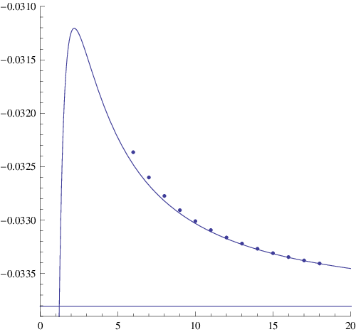
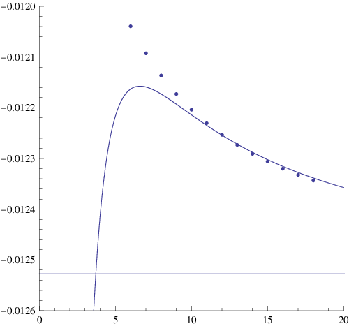
The Lee-Yang model two conformal boundary conditions which are connected by an integrable boundary flow which has been studied in great detail [14]. The model is nonunitary and the boundary field generating the boundary flow has conformal weight $-1/5$ , which means that the perturbation is UV finite but IR divergent. Since $h=-1/5$ , $y=1-h=6/5$ and consequently the leading corrections from truncation errors, which are power series in $n^{-y}$ , decay very rapidly and the TCSA quickly becomes very accurate. The truncation does still have an effect, of course, and the accuracy of the numerical method allows us to check the predictions for the coefficients of $\lambda^{2}$ in the first and second energy gaps. The results are shown in 6, where we show the coefficients extracted from the TCSA method and also the prediction based on the two leading terms in $n^{-y}$ . We see very good agreement so that the leading terms do indeed give the correct behaviour. We have also checked this in the tri-critical Ising model where we also get good agreement, but the corrections from the terms in $n^{-3y}$ are larger.

We have used the following expression for the second energy level in the Lee-Yang model, which is valid for any system where the representation $\psi$ of conformal weight $H$ is degenerate at level 2 and has only a single state at that level which we have chosen to be $L_{-2}{|{\psi}\rangle}$ :

$\displaystyle E_{2}$	$\displaystyle=$	$\displaystyle(H+2)+{\tilde{\lambda}}C^{\prime}\left(1+\frac{4h(h{-}1)}{\mathcal{N}}\right)$
	$\displaystyle+$	$\displaystyle\!\!\!\!({\tilde{\lambda}}C^{\prime})^{2}\left[\frac{2h^{2}}{\mathcal{N}}{+}\frac{h^{2}(2h{-}1)^{2}}{2H\mathcal{N}}{-}\int_{0}^{1}\frac{{\mathrm{d}}z}{z^{y}}\left(F^{2}{-}\frac{4h^{2}}{\mathcal{N}z^{3-y}}{-}\frac{h^{2}(2h-1)^{2}}{(2H\mathcal{N})z^{2-y}}{-}\frac{(4h(h{-}1){+}\mathcal{N})^{2}}{(\mathcal{N})^{2}z^{1-y}}\right)\right]\;,\;\;$
$\displaystyle F^{2}$	$\displaystyle=$	$\displaystyle\frac{1}{\mathcal{N}}\left(\left[z(z^{2}-1)\frac{{\mathrm{d}}}{{\mathrm{d}}z}+(3z^{2}+1)h-2\right]\left[(z-1/z)\frac{{\mathrm{d}}}{{\mathrm{d}}z}+h(3+1/z^{2})\right]+\mathcal{N}\right)F^{0}\;,\;\;$
$\displaystyle F^{0}$	$\displaystyle=$	$\displaystyle\raisebox{-7.11317pt}{\mbox{ $\begin{picture}(3901.0,-2683.0){\put(4800.0,-1860.0){\line{ 0}{-1}{600.0}}}{\put(5700.0,-1860.0){\line{ 0}{-1}{600.0}}}{\put(4200.0,-2460.0){\line{ 1}{ 0}{2100.0}}}\put(4150.0,-2460.0){\pic@makebox@{\makebox}{}(0.0,0.0)[rc]{$\psi$}}\put(4800.0,-1800.0){\pic@makebox@{\makebox}{}(0.0,0.0)[cb]{$\phi$}}\put(4800.0,-2560.0){\pic@makebox@{\makebox}{}(0.0,0.0)[ct]{$1$}}\put(5250.0,-2380.0){\pic@makebox@{\makebox}{}(0.0,0.0)[cb]{$\psi$}}\put(5700.0,-1800.0){\pic@makebox@{\makebox}{}(0.0,0.0)[cb]{$\phi$}}\put(5700.0,-2560.0){\pic@makebox@{\makebox}{}(0.0,0.0)[ct]{$z$}}\put(6400.0,-2460.0){\pic@makebox@{\makebox}{}(0.0,0.0)[lc]{$\psi$}}\end{picture}\;\;$}}\;,\;\;\mathcal{N}=\frac{c}{2}+4H\;,\;\;\;\;$	(6.1)

where for the lee-Yang model $h=H=-1/5$ and

F^{0}=z^{1/5}(1-z)^{2/5}{}_{2}F_{1}({\textstyle\frac{2}{5}},{\textstyle\frac{3}{5}};{\textstyle\frac{4}{5}};z)\;,\;\;C^{\prime}=\left(\frac{\Gamma(1/5)\Gamma(2/5)}{\Gamma(-1/5)\Gamma(4/5)}\right)^{1/2}\;.

(6.2)

7 Fixed points and the coupling constant renormalisation.

One of the principal effects of the coupling constant renormalisation in the TCSA approach is the possibility to move the IR fixed point of the finite-size scaling flow from infinite coupling constant to finite coupling constant. From equations (2.9) and (3.13), we see that for $C$ positive, the IR fixed point at $\lambda_{\infty}=\infty$ is brought to the finite value

\lambda_{n}^{*}=\frac{y\Gamma(h)}{C}(\pi n)^{y}\;,

(7.1)

However, just as the coupling to the identity operator depends on the level of the state, so the coupling constant renormalisation depends on the level of the state, so that the one-loop effective coupling constant renormalisation of a state at level $E$ is not given by (3.12), but rather by

\lambda_{n}^{*}(E)=A(n)(n-E)^{y}\;,

(7.2)

where the one-loop prediction for $A(n)$ is $A(n)=y\Gamma(h)\pi^{y}/C$ . The exact position of the fixed point is not determined very accurately by the 1–loop calculation, (indeed we shall see in section 8.2 that the position of the fixed point in the tri-critical Ising model is approximately $\lambda^{*}_{n}=B\sqrt{n}$ ) but we might conjecture is that the dependence on energy level still has this form. In figure 7(a) we show the full TCSA spectrum for the tri-critical Ising strip with boundary conditions $(12)$ and $(11)$ . The level crossings seen for positive $\lambda$ occur at the IR fixed point, and their position depends on the excitation level. We have also shown a fit to these positions of the form $\lambda_{\mathrm{FP}}(n,E)=A(n)(n-E)^{y}$ . This at least appears to capture the qualitative behaviour quite well.

A second prediction is that the position of this fixed point is independent of the unperturbed boundary condition. In figure 7(b) we show the TCSA spectra of the three strips with one boundary being the perturbation $(12)\to(21)$ and the other being one of the three fixed boundary conditions $(r1)$ . As can be seen, the three spectra agree very well indeed on both the location of the fixed points, indicated by the multiple line degeneracies, on the energy-dependence of these fixed points and on the rescaling of the Hamiltonian, confirming the prediction of our analysis that these effects are independent of the unperturbed boundary condition (to leading order).

8 Flows generated by irrelevant fields

When we consider a flow with a UV and an IR fixed point, we can attempt to describe it in terms of perturbations of either fixed point. A perturbation of an IR fixed point will be by an irrelevant field which is a non-renormalisable perturbation. This means that the perturbation theory will have divergences that require regulation and that a possibly infinite number of counterterms will be required to allow one to remove the regulator. For this reason, they have only infrequently been studied in the literature [18, 19, 20]. In TCSA, however, there is no need to introduce counterterms, one can simply compute the spectrum of the truncated Hamiltonian.

We have investigated this in the case of the tri-critical Ising model. There are three IR fixed points in the basic sequence (9.1). In the case of the $(11)$ and $(31)$ boundary conditions, the fields on the boundary comprise the vacuum representation of the Virasoro algebra so it is expected that the flow will be generated by the field $T(x)$ , the boundary stress-energy tensor, as in [20]; for the $(21)$ boundary condition, the boundary fields form the $(11)$ and $(31)$ representations and it is to be expected that the flow is generated by the field $\phi_{(31)}$ of weight $3/2$ , mirroring the case in the bulk flows considered in [19]. We shall present some results for this last case, and for the flow $(21)\to(13)$ , in particular.

8.1 Comparison with exact results

Firstly, we find that the TCSA spectrum is in very good agreement with the “exact” TBA spectrum; we show the results for the spectrum in figure 11. Secondly, we can compare the TCSA couplings $\lambda^{(21)}_{n}$ at truncation level $n$ with the effective coupling $\lambda^{(13)}_{\infty}$ for the description of the system as a perturbation of the $(13)$ by the field $\phi_{(13)}$ . On dimensional grounds, we expect a relation of the form

\lambda^{(13)}_{\infty}=(\lambda^{(21)}_{n})^{-4/5}g(\lambda^{(21)}_{n}n^{1/2})\;,

(8.1)

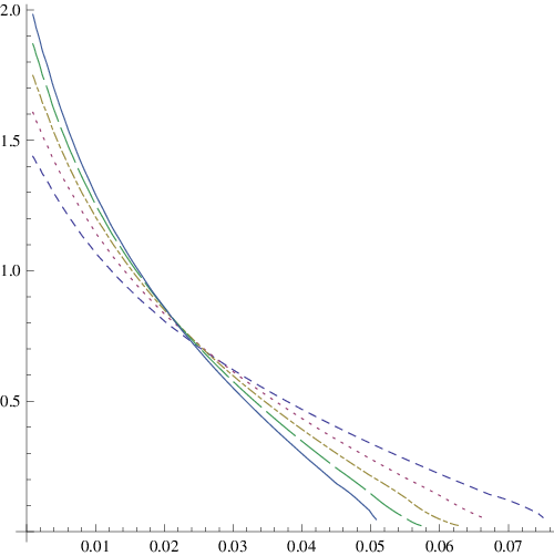
and this indeed what we find. In figure 8(a) we plot the effective couplings against the TCSA coupling for various truncation levels, and in figure 8(b) we plot the scaling function $\lambda^{(13)}_{\infty}(\lambda^{(21)}_{n})^{4/5}$ .

The scaling form (8.1) does, however, have the major consequence that the TCSA coupling constant does not converge to a fixed value as the truncation level is increased. For an irrelevant perturbation, $h>1$ and so $y<0$ . If the function $g(x)$ in (3.12) is approximately equal to one for a range $|x|<A$ , then the TCSA scaling function $g_{n}(\lambda)$ is approximately equal to one for $|\lambda|<An^{-y}$ . For $y$ positive, this range grows with increasing $n$ ; for an irrelevant perturbation it shrinks. In this case, we see that

\lambda^{(13)}_{\infty}(\lambda^{(21)}_{n})^{4/5}\simeq 0.06\;\;\;\;\hbox{for}\;\;\;\;\lambda^{(21)}_{n}<\frac{e^{-3}}{\sqrt{n}}\;.

(8.2)

8.2 Comparison with TCSA parameters

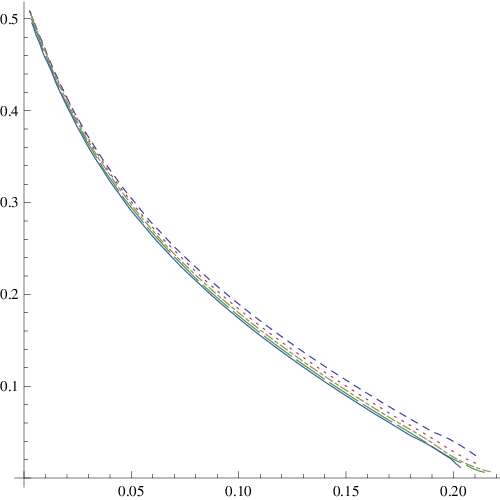
While (8.1) and (8.2) relate the TCSA parameter $\lambda^{(21)}_{n}$ to the “exact” parameter $\lambda^{(13)}_{\infty}$ , it is also interesting to compare the two TCSA parameters. In this case we find the problem that the ranges in which the TCSA parameters are good approximations to the “exact” parameters do not overlap. The IR parameter is good for $\lambda^{(21)}<0.05\,n^{-1/2}$ , which equates to $\lambda^{(13)}>.7n^{2/5}$ , while we can see from figure 4(a) that the UV parameter is good for $\lambda^{(13)}<.5n^{2/5}$ (where we have used the $Z_{2}$ symmetry to relate $\lambda^{(13)}$ to $-\lambda^{(12)}$ .) As a consequence, there are no values of the TCSA coupling constants for which (8.2) holds. Instead we find the interesting plot 9(a); as $n$ increases, the relation between the two TCSA couplings changes. For either of the couplings small, there is an approximate linear relationship. We can elucidate this by noting that the TCSA coupling relation itself takes a scaling form as we show in figure 9(b), where we see that, to a good approximation,

\lambda^{(13)}_{n}\sqrt{n}\simeq F(\lambda^{(21)}_{n}/\sqrt{n})\;,

(8.3)

where

F(x)\simeq 0.5-6.x\;\hbox{for $x$ small,}\qquad F(x)\simeq 0.3-1.3x\;\hbox{for $F(x)$ small}\;.

(8.4)

The linear relation is to be expected, as the perturbing fields at one end (UV or IR) will flow into the perturbing field at the other (IR or UV, respectively) and so the coupling at one end will end up being linearly related to the coupling at the other. Quite why this relation takes the form (8.3) is unclear at the moment.

9 TCSA flows beyond the fixed point

As has been remarked on before [12, 20], the TCSA spectra have the remarkable property that they extend beyond the IR fixed points and can encompass several different perturbative flows. These appear to follow the sequence of flows found first by Lesage et al in [15] and which also appear in Fredenhagen et al [16] and Dorey et al [17] and which in the simplest form applicable to the tri-critical Ising model is

(12)\dashrightarrow(11)\leftarrow(12)\rightarrow(21)\leftarrow(13)\rightarrow(31)\dashleftarrow(13)

(9.1)

where the dashed arrows reflect what is seen in TCSA and are a natural extension of the sequence in the papers cited. The same sequence is seen no matter which boundary condition we take as the starting point from which we perturb. This applies also to the case of irrelevant, non-renormalisable perturbations starting from the ‘fixed’ $(r1)$ boundary conditions. This enables us to put coordinates on the sequence, in the sense that every pair of flows is covered as the standard perturbation of a boundary condition, and we can relate the coupling constants on successive overlapping pairs:

\begin{array}[]{c@{}ccc@{}ccc@{}ccc@{}ccc@{}ccc@{}ccc@{}cccccc}&&&&\lx@intercol\hfil(12)+\mu^{(12)}\phi_{13}\hfil\lx@intercol&\lx@intercol\hfil(13)+\mu^{(13)}\phi_{13}\hfil\lx@intercol&\\ &&&&\lx@intercol\hfil\overbrace{\phantom{1)\;\leftarrow\;(12)\;\rightarrow\;(2}}\hfil\lx@intercol&\lx@intercol\hfil\overbrace{\phantom{1)\;\leftarrow\;(12)\;\rightarrow\;(2}}\hfil\lx@intercol\\[-11.38109pt] (1&2)&\dashrightarrow&(1&1)&\leftarrow&(1&2)&\rightarrow&(2&1)&\leftarrow&(1&3)&\rightarrow&(3&1)&\dashleftarrow&(1&3)\\[-11.38109pt] &\lx@intercol\hfil\underbrace{\phantom{1)\;\leftarrow\;(12)\;\rightarrow\;(2}}\hfil\lx@intercol&\lx@intercol\hfil\underbrace{\phantom{1)\;\leftarrow\;(12)\;\rightarrow\;(2}}\hfil\lx@intercol&\lx@intercol\hfil\underbrace{\phantom{1)\;\leftarrow\;(12)\;\rightarrow\;(2}}\hfil\lx@intercol\\[8.53581pt] &\lx@intercol\hfil(11)+\mu^{(11)}T+..\hfil\lx@intercol&\lx@intercol\hfil(21)+\mu^{(21)}\phi_{31}+..\hfil\lx@intercol&\lx@intercol\hfil(31)+\mu^{(31)}T+..\hfil\lx@intercol\end{array}

(9.2)

where the ellipsis in the perturbations of the fixed boundary conditions shows that further counterterms may be needed as these perturbations are non-renormalisable. As an example of the way the TCSA flows can encompass several fixed points, in figure 10 we show the scaled gaps for the perturbation of the $(21)$ boundary conditions by the irrelevant field $\phi_{(31)}$ of conformal weight $3/2$ . As can be seen, all five fixed points of (9.1) appear.

To give support to this picture, we present the TCSA spectra for the flow $(13)\to(21)$ obtained from the three separate routes: the relevant perturbation of the $(13)$ boundary condition, the irrelevant perturbation of the $(21)$ boundary condition, and the continuation of the flow $(12)\to(21)$ given by the relevant perturbation of the $(12)$ boundary condition. These are all shown in figure 11.

The TBA spectra are given as functions of the boundary reflection parameter $\theta_{B}$ in [21]²² 2 The equations in [15, 21] for the $g$ -function are known not to be correct, but they do describe the changes under a purely boundary perturbation. See [17] for the correct equations when there is a simultaneous bulk perturbation.or $\xi$ of Feverati et al. [8] (note $\xi=\theta_{B})$ . Using the results in [22, 23], we can find the exact expression for $\theta_{B}$ in terms of the perturbative coupling constant $\lambda^{(13)}$ of the relevant perturbation of the $(13)$ boundary condition. We can also find the approximate numerical result for the boundary parameter in terms of the TCSA coupling $\lambda^{(21)}$ , which is only valid for small coupling. These are summarised below

\begin{array}[]{c|ccl}\hbox{Boundary}&&&\hbox{$\theta_{B}$}\\ \hline\cr(13)&&&\left({\textstyle\frac{5}{4}}\log a-\log C_{1}\right)+{\textstyle\frac{5}{2}}\log\lambda^{(13)}\\ &&=&1.96102...+{\textstyle\frac{5}{2}}\log\lambda^{(13)}\\ \hline\cr(21)&&&-5.-2.\log\lambda^{(21)}+\ldots\end{array}

(9.3)

The constants in the first relation are

\displaystyle C_{1}={\textstyle\frac{3}{2}}\pi\left[\Gamma({\textstyle\frac{1}{5}})\right]^{-5}\;,\;\;\;\;a=\frac{{\textstyle\frac{3}{5}}\pi\sin({\textstyle\frac{8}{5}}\pi)}{\Gamma({\textstyle\frac{1}{5}})^{3}\Gamma({\textstyle\frac{7}{5}})\sin({\textstyle\frac{12}{5}}\pi)\sin({\textstyle\frac{4}{5}}\pi)}\;.

(9.4)

Finally, we have also found an approximate numerical relation between the couplings $\lambda^{(21)}$ and $\lambda^{(12)}$ for this region, which is

\frac{\lambda^{(12)}_{n}}{\sqrt{n}}-8.\sqrt{n}\lambda^{(21)}_{n}\simeq 0.5\;,

(9.5)

which is in agreement with (8.4) to the accuracy that is obtainable for the flow from the $(12)$ boundary condition beyond the $(21)$ fixed point.

10 Conclusions

We have made further progress in understanding the errors in the truncated conformal space approach to perturbed boundary conformal field theory on a strip. The principal quantity calculated with TCSA is the spectrum as a function of the coupling constant. The errors are of two principal sorts - a renormalisation of the coupling constant and a change in the energy scale. We have found perturbative expressions for these from physical arguments and showed they are correct using an analysis of the perturbative spectrum.

One important aspect of these predictions is that they are independent of the second boundary condition on the strip and we have verified this by considering different choices for the unperturbed boundary condition and finding the same results for each choice.

Furthermore we have investigated the behaviour of the TCSA spectrum for large coupling constant. We have reported before that this appears to show a sequence of RG flows in the same pattern as found by Lesage et al [15], and we know show that this is quantitatively correct as well, in the case of the tri-critical Ising model.

It would be good to find some way to describe the full RG flows such as in figure 10 in terms of some beta-function which has the sequence of fixed points as its zeroes, but at the moment we are unsure how to do that. In the lattice model, the perturbation parameter is a boundary magnetic field and the sequence of fixed points (9.1) (excluding the points joined by the dashed lines) can be found simply by varying this field [24]; of course in the quantum model this is not simply the case - the natural sequence of flows splits up into overlapping pairs of flows in both the TBA and the TCSA descriptions. It may be helpful to use the coordinates on the full moduli space given by the values of the $g$ -function and the excited $g$ -function which corresponds to the overlap with the bulk spin field. This is something we hope to return to shortly,

Finally the ideas on the perturbative treatment of the corrections to the TCSA presented here can be easily adapted to the case of bulk flows which we plan to address in [25].

11 Acknowledgements

I am very grateful to G. Feverati, F. Ravanini and P.A. Pearce for providing the numerical data for the TBA flows from their papers [7, 8], without which this paper would not have been possible.

I would like to thank P. Giokas, G. Takács and G.Zs. Tóth for helpful discussions, B. Doyon and G. Takács for comments on the manuscript and STFC grant ST/G000395/1 for support. All numerical calculations were performed using Mathematica [26].

References

- [1] V.P. Yurov and A.B. Zamolodchikov, Truncated conformal space approach to the scaling Lee-Yang model, Int. J. Mod. Phys A5 (1990) 3221–3245.
- [2] R.M. Konik and Y. Adamov, A Numerical Renormalization Group for Continuum One-Dimensional Systems, cond-mat/0701605
- [3] G.P. Brandino, R.M. Konik and G. Mussardo, Energy level distribution of perturbed conformal field theories , J. Stat. Mech. (2010)P07013, arXiv:1004.4844
- [4] M. Lässig, G. Mussardo and J.L. Cardy, The scaling region of the tricritical Ising model in two dimensions , Nucl. Phys. B 348 (1991) 591-618.
- [5] I. Affleck, Edge critical behaviour of the two-dimensional tri-critical Ising model, J. Phys. A33 (2000) 6473-6479 [cond-mat/0005286].
- [6] K. Graham and G.M.T. Watts, Defect lines and boundary flows, JHEP 0404 (2004) 019 [hep-th/0306167].
- [7] G. Feverati, P.A. Pearce and F. Ravanini, Excited Boundary TBA in the Tricritical Ising Model, Int. J. Mod. Phys. A19S2 (2004) 155-167 [hep-th/0306196]
- [8] G. Feverati, P.A. Pearce and F. Ravanini, Exact boundary flows in the tricritical Ising model, Nucl. Phys. B 675 (2003) 469-515 [hep-th/0308075]
- [9] G. Feverati, Exact boundary flow in the tricritical Ising model, J. Stat. Mech.0403: P001,2004 [hep-th/0312201]
- [10] J.L. Cardy, Boundary conditions, fusion rules and the Verlinde formula, Nucl. Phys. B 324 (1989) 581–596.
- [11] L. Chim, Boundary S-matrix for the Tricritical Ising Model, Int. J. Mod. Phys. A11 (1996) 4491, hep-th/9510008v1
- [12] G. Feverati1, K. Graham, P.A. Pearce, G.Zs. Tóth and G.M.T. Watts, A renormalisation group for the truncated conformal space approach, J. Stat. Mech. (2008) P03011 [hep-th/0612203]
- [13] J.L. Cardy, Conformal Invariance and Statistical Mechanics, in Exact Methods in Low-Dimensional Statistical Physics and Quantum Computing, Les Houches lectures 2008, [arXiv:0807.3472]
- [14] P. Dorey, A. Pocklington, R. Tateo and G. Watts, TBA and TCSA with boundaries and excited states, Nucl. Phys. B 525 (1998) 641 [hep-th/9712197].
- [15] F Lesage, H. Saleur and P. Simonetti, Boundary flows in minimal models, Phys. Lett. B427 (1998) 85–92, hep-th/9802061.
- [16] S. Fredenhagen, M.R. Gaberdiel and C. Schmidt-Colinet, Bulk flows in Virasoro minimal models with boundaries, J. Phys. A42:495403, 2009, arXiv:0907.2560
- [17] P. Dorey, R. Tateo and R. Wilbourne, Exact g-function flows from the staircase model, Nucl. Phys. B 843 (2011) 724-752, arXiv:1008.1190
- [18] Al.B. Zamolodchikov, From tricritical Ising to critical Ising by thermodynamic Bethe ansatz, Nucl. Phys. B 358 (1991) 524–546
- [19] G. Feverati, E. Quattrini and F. Ravanini, Infrared Behaviour of Massless Integrable Flows entering the Minimal Models from , Phys. Lett. B374 (1996) 64-70, hep-th/9512104v2
- [20] G.Zs Tóth, A study of truncation effects in boundary flows of the Ising model on a strip, J. Stat. Mech. (2007) P04005, hep-th/0612256
- [21] R.I. Nepomechie and C. Ahn, TBA boundary flows in the tricritical Ising field theory, Nucl. Phys. B 647 (2002) 433-470, hep-th/0207012
- [22] V.V. Bazhanov, S.L. Lukyanov and Al.B. Zamolodchikov, Integrable structure of conformal field theory, quantum KdV theory and thermodynamic Bethe ansatz, Commun. Math. Phys. 177 (1996) 381-398, hep-th/9412229
- [23] V.V. Bazhanov, S.L. Lukyanov and Al.B. Zamolodchikov, Integrable quantum field theories in finite volume: Excited state energies, Nucl. Phys. B 489 (1997) 487-531, hep-th/9607099
- [24] P. Giokas, Mean field theory for boundary Ising and tri-critical Ising models, preprint kcl-mth-11-05.
- [25] P. Giokas and G.M.T. Watts, in preparation.
- [26] Wolfram Research Inc, Mathematica, version 8.0, Champaign Illinois, 2010.