跳到论文正文
W Papers独立论文阅读器 arXiv:1104.0136 论文正文 计算阅读时间 · 0%
引用这篇论文根据当前论文元数据生成,正式投稿前建议核对。


License: arXiv.org perpetual non-exclusive license
arXiv:1104.0136v1 [cs.IT] 01 Apr 2011

On Interference Alignment and the Deterministic Capacity for Cellular Channels with Weak Symmetric Cross Links

Jörg Bühler Affiliation: Heinrich-Hertz-Lehrstuhl für Informationstheorie
und theoretische Informationstechnik
Technische Universität Berlin
Einsteinufer 25, D-10587 Berlin, Germany
Email: joerg.buehler@mk.tu-berlin.de
   Gerhard Wunder Affiliation: Fraunhofer Heinrich Hertz Institute
Einsteinufer 37, D-10587 Berlin, Germany
Email: gerhard.wunder@hhi.fraunhofer.de
Abstract

In this paper, we study the uplink of a cellular system using the linear deterministic approximation model, where there are two users transmitting to a receiver, mutually interfering with a third transmitter communicating with a second receiver. We give an achievable coding scheme and prove its optimality, i.e. characterize the capacity region. This scheme is a form of interference alignment which exploits the channel gain difference of the two-user cell.

††footnotetext: This research is supported by Deutsche Forschungsgemeinschaft (DFG) under grant WU 598/1-2.

I Introduction

In recent years, approximate characterizations of capacity regions of multi-user systems have gained more and more attention, with one of the most prominent examples being the characterization of the capacity of the Gaussian interference channel to within one bit/s/Hz in [1]. One of the tools that arised in the context of capacity approximations and has been shown to be useful in many cases is the linear deterministic model introduced in [2] [3]. Here, the channel is modelled as a deterministic mapping that operates on bit vectors and mimics the effect the physical channel and interfering signals have on the binary expansion of the transmitted symbols. Basically, the effect of the channel is to erase a certain number of ingoing bits, while superposition of signals is given by the modulo addition. Even though this model deemphasizes the effect of thermal noise, it is able to capture some important basic features of wireless systems, namely the superposition and broadcast properties of electromagnetic wave propagation. Hence, in multi-user systems where interference is one of the most important limiting factors on system performance, the model can also be useful to devise effective coding and interference mitigation techniques. There are many examples where a linear deterministic analysis can be successfully carried over to coding schemes for the physical (Gaussian) models or be used for approximative capacity or degrees of freedom determination. Among them are results concerning the the two-user interference channel [4], the KK-user interference channel [5], the XX-channel [6], fading broadcast channels without channel state information at the transmitter [7], many-to-one and one-to-many interference channels [8], cooperative interference channels [9, 10] and cyclically symmetric deterministic interference channels [11]. Here, the optimal transmission schemes often involve interference alignment, where the transmitted signals are designed such that at the receivers, the undesired part of the signal that is due to the different interfering signals aligns in a certain subspace of the receive space.

Contributions. From a practical viewpoint, cellular systems are of major interest. Generally, a cellular system consists of a set of base stations each communicating with a distinct set of (mobile) users. Effective coding and interference mitigation schemes are still an active area of research. Approximative models such as the linear deterministic approach might help to gain more insight into these problems. In this paper, we take a step into this direction and investigate a cellular setup using the linear deterministic model. To our knowledge, this is the first linear deterministic capacity analysis for cellular-type channels. We determine the capacity region and the corresponding optimal coding scheme. This scheme involves a form of interference alignment, exploiting the channel gain difference of the two-user cell.

Organization. The paper is organized as follows: Section II introduces the system model. In section III, we give an achievable rate region and the corresponding communication scheme, which essentially uses the principle of interference alignment. In section IV, we prove that this region actually constitutes the capacity region by deriving an outer bound region that coincides with the achievable rate region. Finally, section V concludes the paper.

Notation. Throughout the paper, 𝔽2={0,1}\mathbb{F}_{2}=\{0,1\} denotes the binary finite field, for which addition is written as ⊕\oplus, which is addition modulo 2. For two matrices A∈𝔽2nA×mA\in\mathbb{F}_{2}^{n_{A}\times m} and B∈𝔽2nB×mB\in\mathbb{F}_{2}^{n_{B}\times m}, we denote by [A;B]∈𝔽2nA+nB×m[A;B]\in\mathbb{F}_{2}^{n_{A}+n_{B}\times m} the matrix that is obtained by stacking AA over BB. Moreover, for a sequence of matrices A1,…,AnA_{1},\ldots,A_{n}, we write (Ak)k=1n(A_{k})_{k=1}^{n} for the stacked matrix, i.e. (Ak)k=1n=[(Ak)k=1n−1;An](A_{k})_{k=1}^{n}=[(A_{k})_{k=1}^{n-1};A_{n}]. Similarily, [A|B][A|B] stands for placing AA next to BB. The zero matrix of size m×nm\times n and the matrix with all entries equal to one are denoted by 𝟎m×n\mathbf{0}_{m\times n} and 𝟏m×n\mathbf{1}_{m\times n}, respectively. Furthermore, 𝟏m=𝟏m×1\mathbf{1}_{m}=\mathbf{1}_{m\times 1}, 𝟎m=𝟎m×1\mathbf{0}_{m}=\mathbf{0}_{m\times 1} and InI_{n} is the n×nn\times n identity matrix. For a matrix A∈𝔽2m×nA\in\mathbb{F}_{2}^{m\times n}, we write |A||A| for the number of ones in AA. Finally, div and mod denote integer division and the modulo operation, respectively, where we use the convention x​ div ​0=0x\text{~div~}0=0.

II System Model

Refer to caption
Fig. 1: System model.

The system we consider here represents a basic version of the uplink of cellular system and consists of three transmitters (mobile users) T​x1,T​x2Tx_{1},Tx_{2} and T​x3Tx_{3} and two receivers (base stations) R​x1,R​x2Rx_{1},Rx_{2} (c.f. Figure 1). The system is modelled using the linear deterministic model [2, 3]. Here, the input symbol at transmitter T​xiTx_{i} is given by a bit vector Xi∈𝔽2qX_{i}\in\mathbb{F}_{2}^{q} and the output bit vectors YjY_{j} at R​xjRx_{j} are deterministic functions of the inputs: Defining the shift matrix S∈𝔽2q×qS\in\mathbb{F}_{2}^{q\times q} by

S=(000⋯0100⋯0010⋯0⋱⋱⋱0⋯010),S=\begin{pmatrix}0&0&0&\cdots&0\\ 1&0&0&\cdots&0\\ 0&1&0&\cdots&0\\ \vdots&\ddots&\ddots&\ddots&\vdots\\ 0&\cdots&0&1&0\\ \end{pmatrix}, (1)

the input/output equations of the system are given by

Y1\displaystyle Y_{1} =\displaystyle= Sq−n11​X1⊕Sq−n12​X2⊕Sq−n13​X3,\displaystyle S^{q-n_{11}}X_{1}\oplus S^{q-n_{12}}X_{2}\oplus S^{q-n_{13}}X_{3}, (2)
Y2\displaystyle Y_{2} =\displaystyle= Sq−n21​X1⊕Sq−n22​X2⊕Sq−n23​X3.\displaystyle S^{q-n_{21}}X_{1}\oplus S^{q-n_{22}}X_{2}\oplus S^{q-n_{23}}X_{3}.

Here, qq is chosen arbitrarily such that q≥maxi,j​{ni​j}q\geq\text{max}_{i,j}\{n_{ij}\}. Note that ni​jn_{ij} gives the number of bits that can be passed over the channel between T​xjTx_{j} and R​xiRx_{i}, i.e. ni​jn_{ij} represent channel gains. There are three messages to be transmitted in the system: Wi​jW_{ij} denotes the message from transmitter T​xjTx_{j} to the intended receiver R​xiRx_{i}. The definitions of (block) codes, error probability, achievable rates and the capacity region are according to the standard information-theoretic definitions. For the remainder of the paper, the transmission rate corresponding to message W11W_{11} is represented by R1R_{1}, the rate corresponding to W12W_{12} by R2R_{2} and the rate for W23W_{23} by R3R_{3}.

In the following, we assume without loss of generality that n11≥n12n_{11}\geq n_{12} and write n1=n11,n2=n12,n3=n23,nD=n13n_{1}=n_{11},n_{2}=n_{12},n_{3}=n_{23},n_{D}=n_{13} and Δ=n1−n2\Delta=n_{1}-n_{2}. In this paper, we further restrict ourselves to the case n21=n22=:nMn_{21}=n_{22}=:n_{M}, to which we refer to as symmetric MAC interference and assume the weak interference condition nD+nM≤min​{n2,n3}n_{D}+n_{M}\leq\text{min}\left\{n_{2},n_{3}\right\}. Also, we may choose q=max​{n1,n3}q=\text{max}\{n_{1},n_{3}\}.

III An Achievable Region

In this section, we derive an achievable rate region. For this, we split the system into two subsystems and derive achievable regions for each of them, denoted as ℛach(1)\mathcal{R}^{(1)}_{\text{ach}} and ℛach(2)\mathcal{R}^{(2)}_{\text{ach}},¡ respectively. The sum of these two regions then results in an achievable region ℛach\mathcal{R}_{\text{ach}} for the overall system. We begin by considering the two subsystems and the corresponding achievable rate regions. The first system is given by the equations

Y1(1)\displaystyle Y_{1}^{(1)} =\displaystyle= Sq(1)−n1(1)​X1(1)⊕Sq(1)−n1(1)​X2(1)⊕Sq(1)−nD​X3(1),\displaystyle S^{q^{(1)}-n_{1}^{(1)}}X_{1}^{(1)}\oplus S^{q^{(1)}-n_{1}^{(1)}}X_{2}^{(1)}\oplus S^{q^{(1)}-n_{D}}X_{3}^{(1)},\quad\,\, (3)
Y2(1)\displaystyle Y_{2}^{(1)} =\displaystyle= Sq(1)−n3(1)​X3(1),\displaystyle S^{q^{(1)}-n_{3}^{(1)}}X_{3}^{(1)},

where n1(1)=n2−nM,n3(1)=n3−nMn_{1}^{(1)}=n_{2}-n_{M},n_{3}^{(1)}=n_{3}-n_{M} and q(1)=max​{n1(1),n3(1)}q^{(1)}=\text{max}\{n_{1}^{(1)},n_{3}^{(1)}\}. The second system is defined by

Y1(2)\displaystyle Y_{1}^{(2)} =\displaystyle= Sq(2)−n1(2)​X1(2)⊕Sq(2)−n2(2)​X2(2),\displaystyle S^{q^{(2)}-n_{1}^{(2)}}X_{1}^{(2)}\oplus S^{q^{(2)}-n_{2}^{(2)}}X_{2}^{(2)}, (4)
Y2(2)\displaystyle Y_{2}^{(2)} =\displaystyle= Sq(2)−nM​X1(2)⊕Sq(2)−nM​X2(2)⊕Sq−nM​X3(2),\displaystyle S^{q^{(2)}-n_{M}}X_{1}^{(2)}\oplus S^{q^{(2)}-n_{M}}X_{2}^{(2)}\oplus S^{q-n_{M}}X_{3}^{(2)},

with q(2)=n1(2)=nM+Δq^{(2)}=n_{1}^{(2)}=n_{M}+\Delta and n2(2)=nMn_{2}^{(2)}=n_{M}. Note that this split is possible due to the weak interference condition nD+nM≤min​{n2,n3}n_{D}+n_{M}\leq\text{min}\left\{n_{2},n_{3}\right\}. The corresponding transmitters and receiver are denoted as T​x1(1),R​x1(1)Tx_{1}^{(1)},Rx_{1}^{(1)} etc. Figure 2 illustrates the split of the system. Here, the bars represent the bit vectors as seen at the two receivers; the zero parts due to the channel shifts are not displayed.

We define ℛach(1)\mathcal{R}^{(1)}_{\text{ach}} as the set of points (R1(1),R2(1),R3(1))\left(R^{(1)}_{1},R^{(1)}_{2},R^{(1)}_{3}\right) satisfying

R3(1)\displaystyle R^{(1)}_{3} ≤\displaystyle\leq n3(1)\displaystyle n^{(1)}_{3} (5)
R1(1)+R2(1)\displaystyle R^{(1)}_{1}+R^{(1)}_{2} ≤\displaystyle\leq n1(1)\displaystyle n^{(1)}_{1} (6)
R1(1)+R2(1)+R3(1)\displaystyle R^{(1)}_{1}+R^{(1)}_{2}+R^{(1)}_{3} ≤\displaystyle\leq n2+n3−nD−2​nM.\displaystyle n_{2}+n_{3}-n_{D}-2n_{M}. (7)

Similarily, ℛach(2)\mathcal{R}^{(2)}_{\text{ach}} is defined by the set of equations

R1(2)+R2(2)\displaystyle R^{(2)}_{1}+R^{(2)}_{2} ≤\displaystyle\leq n1(2)\displaystyle n_{1}^{(2)} (8)
R1(2)+R3(2)\displaystyle R^{(2)}_{1}+R^{(2)}_{3} ≤\displaystyle\leq n1(2)\displaystyle n_{1}^{(2)} (9)
R2(2)+R3(2)\displaystyle R^{(2)}_{2}+R^{(2)}_{3} ≤\displaystyle\leq nM\displaystyle n_{M} (10)
R1(2)+R2(2)+R3(2)\displaystyle R^{(2)}_{1}+R^{(2)}_{2}+R^{(2)}_{3} ≤\displaystyle\leq nM+φ⁡(nM,Δ).\displaystyle n_{M}+\varphi(n_{M},\Delta). (11)

Here, the function φ\varphi for p,q∈ℕ0p,q\in\mathbb{N}_{0} is defined as

φ⁡(p,q)={q+l⁡(p,q)​q2,if​l​(p,q)​is evenp−(l⁡(p,q)−1)​q2,if​l​(p,q)​is odd.\varphi(p,q)=\begin{cases}q+\frac{l(p,q)q}{2},&\mbox{if}\;\;l(p,q)\;\;\mbox{is even}\\ p-\frac{(l(p,q)-1)q}{2},&\mbox{if}\;\;l(p,q)\;\;\mbox{is odd}.\end{cases} (12)

where l⁡(p,q)=p​ div ​ql(p,q)=p\text{~div~}q (note that 00 is considered an even number).

Refer to caption
Fig. 2: Illustration of the split of the system.
Refer to caption
Fig. 3: Example for optimal bit level assignment: The MAC interference aligns at receiver R​x2(2)Rx_{2}^{(2)}.

We now show that the rate regions ℛach(1)\mathcal{R}^{(1)}_{\text{ach}} and ℛach(2)\mathcal{R}^{(2)}_{\text{ach}} are achievable in the respective subsystems. Both regions can be achieved by an orthogonal bit level assignment (and possibly time-sharing). More precisely, for each transmitter, a set of bit levels to be used for data transmission is specified such that at the intended receiver, there is no overlap of these levels with levels used by any other transmitter.

In this way, the achievability of the points in ℛach(1)\mathcal{R}^{(1)}_{\text{ach}} follows directly from the results on the interference channel: If we first consider the one-sided interference channel obtained by removing transmitter T​x2(1)Tx_{2}^{(1)}, the points (RΣ(1),R3(1))\left(R_{\Sigma}^{(1)},R_{3}^{(1)}\right) with R3(1)≤n3(1),RΣ(1)≤n1(1),RΣ(1)+R3(1)≤n2+n3−nD−2​nMR_{3}^{(1)}\leq n^{(1)}_{3},R_{\Sigma}^{(1)}\leq n^{(1)}_{1},R_{\Sigma}^{(1)}+R^{(1)}_{3}\leq n_{2}+n_{3}-n_{D}-2n_{M} can be achieved in this one-sided interference channel using orthogonal coding, which follows from the results in [4]. The same rates can be achieved for the interference channel obtained by removing T​x1(1)Tx_{1}^{(1)}. Then, since the signals X1(1)X_{1}^{(1)} and X2(1)X_{2}^{(1)} are shifted by the same amount at the first receiver, it is clear that in system 1, we can achieve R1(1)R_{1}^{(1)} and R1(2)R_{1}^{(2)} such that R1(1)+R2(1)≤RΣ(1)R_{1}^{(1)}+R_{2}^{(1)}\leq R_{\Sigma}^{(1)}, which implies the achievability of region ℛach(1)\mathcal{R}^{(1)}_{\text{ach}}.

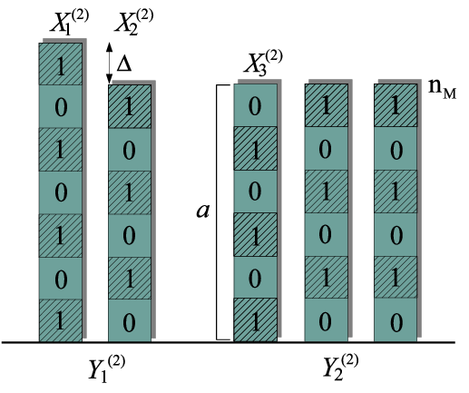
To show the achievability of ℛach(2)\mathcal{R}^{(2)}_{\text{ach}}, let a∈𝔽2nMa\in\mathbb{F}_{2}^{n_{M}} specify the levels used for encoding message W23W_{23} (note that it suffices to specify the first nMn_{M} levels since the others are erased by the channel anyway), where ai=1a_{i}=1 if level ii is used and ai=0a_{i}=0 otherwise. Define γ⁡(a):=𝟏nM−a\gamma(a):=\mathbf{1}_{n_{M}}-a, γ1​(a):=[γ⁡(a);𝟏Δ]\gamma_{1}(a):=[\gamma(a);\mathbf{1}_{\Delta}] and γ2​(a):=[𝟎Δ;γ⁡(a)]\gamma_{2}(a):=[\mathbf{0}_{\Delta};\gamma(a)]. Then we can achieve R3(2)=|a|R_{3}^{(2)}=|a| and all rates R1(2),R2(2)R_{1}^{(2)},R_{2}^{(2)} with R1(2)≤|γ1​(a)|=nM+Δ−|a|,R2(2)≤|γ2​(a)|=nM−|a|R_{1}^{(2)}\leq|\gamma_{1}(a)|=n_{M}+\Delta-|a|,R_{2}^{(2)}\leq|\gamma_{2}(a)|=n_{M}-|a| and R1(2)+R2(2)≤|γ1​(a)|+|γ2​(a)|−ρ⁡(|a|)R_{1}^{(2)}+R_{2}^{(2)}\leq|\gamma_{1}(a)|+|\gamma_{2}(a)|-\rho(|a|), where ρ(x):=mina∈𝔽2nM:|a|=xγ1(a)Tγ2(a).\rho(x):=\underset{a\in\mathbb{F}_{2}^{n_{M}}:|a|=x}{\text{min}}~\gamma_{1}(a)^{T}\gamma_{2}(a). Here, γ1​(a)\gamma_{1}(a) and [γ⁡(a);𝟎Δ][\gamma(a);\mathbf{0}_{\Delta}] specify the levels used by transmitters T​x1(2)Tx_{1}^{(2)} and T​x2(2)Tx_{2}^{(2)}, respectively, except for the ρ⁡(|a|)\rho(|a|) positions that cause an overlap of a level in the received bit vectors γ1​(a)\gamma_{1}(a) and γ2​(a)\gamma_{2}(a), for which one of the positions is exclusively assigned to T​x1(2)Tx_{1}^{(2)} or T​x2(2)Tx_{2}^{(2)}. An assignment vector aa solving the minimization for ρ\rho for a given xx can be shown to be of the form described in the following. Let l=nM​ div ​Δl=n_{M}\text{~div~}\Delta and Q=nM​ mod ​ΔQ=n_{M}\text{~mod~}\Delta, i.e. nM=l​Δ+Qn_{M}=l\Delta+Q. We subdivide aa into l​Δl\Delta subsequences (blocks) of length Δ\Delta and one remainder block of length QQ. We distribute ones over aa until xx entries in aa have been set to 11: We start with the even-numbered blocks, followed by the remainder block. If ll is even, we finally distribute over the odd-numbered blocks. If ll is odd, we also fill the odd-numbered blocks, but in reversed (decreasing) order. To be precise, we define for the case that ll is even

Aeven\displaystyle A_{\text{even}} =\displaystyle= (𝟎1×l2,ek)k=1l/2⊗IΔ,\displaystyle\left(\mathbf{0}_{1\times\frac{l}{2}};e_{k}\right)_{k=1}^{l/2}\otimes I_{\Delta}, (13)
Aodd\displaystyle A_{\text{odd}} =\displaystyle= (ek,𝟎1×l2)k=1l/2⊗IΔ\displaystyle\left(e_{k};\mathbf{0}_{1\times\frac{l}{2}}\right)_{k=1}^{l/2}\otimes I_{\Delta} (14)

and

Aeven\displaystyle A_{\text{even}} =\displaystyle= [(𝟎1×(l−1)2,ek)k=1(l−1)/2;𝟎1×l−12]⊗IΔ,\displaystyle\left[\left(\mathbf{0}_{1\times\frac{(l-1)}{2}};e_{k}\right)_{k=1}^{(l-1)/2};\mathbf{0}_{1\times\frac{l-1}{2}}\right]\otimes I_{\Delta}, (15)
Aodd\displaystyle A_{\text{odd}} =\displaystyle= Ml​Δ​([(ek,𝟎1×(l+1)2)k=1(l−1)/2;el+12]⊗IΔ)\displaystyle M_{l\Delta}\left(\left[\left(e_{k};\mathbf{0}_{1\times\frac{(l+1)}{2}}\right)_{k=1}^{(l-1)/2};e_{\frac{l+1}{2}}\right]\otimes I_{\Delta}\right) (16)

for odd ll. Here, ⊗\otimes denotes the Kronecker product, eke_{k} the unit row vector of appropriate size with 11 at position kk and MN=(eN−k+1)k=1NM_{N}=(e_{N-k+1})_{k=1}^{N} is the flip matrix. Then, defining P=[Aeven​|𝟎l​Δ×Q|​Aodd],P=\left[A_{\text{even}}|\mathbf{0}_{l\Delta\times Q}|A_{\text{odd}}\right], we obtain an optimal assignment aa by setting a=P⁡[𝟏x;𝟎nM−x]a=P[\mathbf{1}_{x};\mathbf{0}_{n_{M}-x}].

We remark that this assignment is not the unique optimal one. Furthermore, it can be interpreted as interference alignment at the receiver R​x2(2)Rx_{2}^{(2)}: The bit levels are chosen such that the interference caused by X1(2)X^{(2)}_{1} and X2(2)X^{(2)}_{2} (MAC interference) aligns at R​x2(2)Rx_{2}^{(2)} as much as possible in the levels that are unused by X3(2)X^{(2)}_{3}. Figure 3 displays the optimal assignment for the case l=6,Q=0l=6,Q=0 and x=R3(2)=3​Δx=R_{3}^{(2)}=3\Delta. The rates achieved here for the first two transmitters are R1(2)=4​ΔR_{1}^{(2)}=4\Delta and R2(2)=3​ΔR_{2}^{(2)}=3\Delta. The optimal assignment described above for the case ll even results in the following form of the function ρ\rho:

ρ⁡(x)={nM−2​x,if​  0≤x≤l​Δ2Q+l​Δ2−x,if​l​Δ2≤x≤l​Δ2+Q0,if​l​Δ2+Q≤x≤nM.\rho(x)=\begin{cases}n_{M}-2x,&\mbox{if}\;\;0\leq x\leq\frac{l\Delta}{2}\\ Q+\frac{l\Delta}{2}-x,&\mbox{if}\;\;\frac{l\Delta}{2}\leq x\leq\frac{l\Delta}{2}+Q\\ 0,&\mbox{if}\;\;\frac{l\Delta}{2}+Q\leq x\leq n_{M}.\end{cases} (17)

In the case that ll is odd, we similarily obtain

ρ⁡(x)={nM−2​x,if​  0≤x≤Q+Δ⁡(l−1)2Δ⁡(l+1)2−x,if​Q+Δ⁡(l−1)2≤x≤Δ⁡(l+1)20,if​Δ⁡(l+1)2≤x≤nM\rho(x)=\begin{cases}n_{M}-2x,&\mbox{if}\;\;0\leq x\leq Q+\frac{\Delta(l-1)}{2}\\ \frac{\Delta(l+1)}{2}-x,&\mbox{if}\;\;Q+\frac{\Delta(l-1)}{2}\leq x\leq\frac{\Delta(l+1)}{2}\\ 0,&\mbox{if}\;\;\frac{\Delta(l+1)}{2}\leq x\leq n_{M}\end{cases} (18)

From this, it is easy to verify that all points in ℛach(2)\mathcal{R}^{(2)}_{\text{ach}} are achievable.

Finally, we obtain an achievable region ℛach=ℛach(1)+ℛach(2)\mathcal{R}_{\text{ach}}=\mathcal{R}^{(1)}_{\text{ach}}+\mathcal{R}^{(2)}_{\text{ach}} for the overall system. This sum region can be, for example, computed by employing Fourier-Motzkin elimination. The resulting region is stated in the following Proposition:

Proposition 1

An achievable region ℛach\mathcal{R}_{\text{ach}} is given by the set of points (R1,R2,R3)∈ℝ3(R_{1},R_{2},R_{3})\in\mathbb{R}^{3} satisfying the constraints

R1\displaystyle R_{1} ≤\displaystyle\leq n1\displaystyle n_{1} (19)
R2\displaystyle R_{2} ≤\displaystyle\leq n2\displaystyle n_{2} (20)
R3\displaystyle R_{3} ≤\displaystyle\leq n3\displaystyle n_{3} (21)
R1+R2\displaystyle R_{1}+R_{2} ≤\displaystyle\leq n1\displaystyle n_{1} (22)
R1+R3\displaystyle R_{1}+R_{3} ≤\displaystyle\leq n1+n3−nD−nM\displaystyle n_{1}+n_{3}-n_{D}-n_{M} (23)
R2+R3\displaystyle R_{2}+R_{3} ≤\displaystyle\leq n2+n3−nD−nM\displaystyle n_{2}+n_{3}-n_{D}-n_{M} (24)
R1+R2+R3\displaystyle R_{1}+R_{2}+R_{3} ≤\displaystyle\leq n2+n3−nD−nM+φ⁡(nM,Δ)\displaystyle n_{2}+n_{3}-n_{D}-n_{M}+\varphi(n_{M},\Delta)~ (25)
R1+R2+2​R3\displaystyle R_{1}+R_{2}+2R_{3} ≤\displaystyle\leq n1+2​n3−nD−nM.\displaystyle n_{1}+2n_{3}-n_{D}-n_{M}. (26)

IV Capacity Region

In this section, we show that the achievable region ℛach\mathcal{R}_{\text{ach}} from the previous section actually constitutes the capacity region 𝒞\mathcal{C}. For the proof, we need the following Lemma:

Lemma 1

For two independent random matrices A,B∈𝔽2n+Δ×mA,B\in\mathbb{F}_{2}^{n+\Delta\times m} with m,n,Δ∈ℕm,n,\Delta\in\mathbb{N}, it holds that

H⁡(A⊕SΔ​B)−H⁡(SΔ​A⊕SΔ​B)\displaystyle H(A\oplus S^{\Delta}B)-H(S^{\Delta}A\oplus S^{\Delta}B) ≤\displaystyle\leq m​φ​(n,Δ),\displaystyle m\varphi(n,\Delta), (27)
H⁡(A⊕SΔ​B)−2​H​(SΔ​A⊕SΔ​B)\displaystyle H(A\oplus S^{\Delta}B)-2H(S^{\Delta}A\oplus S^{\Delta}B) ≤\displaystyle\leq m​Δ.\displaystyle m\Delta. (28)
Proof:

In order to show (27), we let l=n​div​Δ,Q=n​mod​Δl=n~\text{div}~\Delta,Q=n~\text{mod}~\Delta and introduce the following labels for blocks of rows of the matrices AA and BB: A=[S;(Ak)k=1l+1],B=[T;(Bk)k=1l+1]A=[S;(A_{k})_{k=1}^{l+1}],B=[T;(B_{k})_{k=1}^{l+1}], where S,T∈𝔽2Q×mS,T\in\mathbb{F}_{2}^{Q\times m} and Ak,Bk∈𝔽2Δ×mA_{k},B_{k}\in\mathbb{F}_{2}^{\Delta\times m}. Then the shifted versions of AA and BB are SΔ​A=[𝟎Δ×m;S;(Ak)k=1l],SΔ​B=[𝟎Δ×m;T;(Bk)k=1l].S^{\Delta}A=[\mathbf{0}_{\Delta\times m};S;(A_{k})_{k=1}^{l}],S^{\Delta}B=[\mathbf{0}_{\Delta\times m};T;(B_{k})_{k=1}^{l}]. First consider the case that ll is even. Then we have

H⁡(A⊕SΔ​B)−H⁡(SΔ​A⊕SΔ​B)\displaystyle H(A\oplus S^{\Delta}B)-H(S^{\Delta}A\oplus S^{\Delta}B) (29)
=H⁡[S;A1⊕[𝟎Δ−Q×m;T];(Ak+1⊕Bk)k=1l]\displaystyle\,\,\,\,\,=H\left[S;A_{1}\oplus[\mathbf{0}_{\Delta-Q\times m};T];(A_{k+1}\oplus B_{k})_{k=1}^{l}\right]
−H⁡[S⊕T;(Ak⊕Bk)k=1l]\displaystyle\,\,\,\,\,\,\,\,\,\,\,-H\left[S\oplus T;(A_{k}\oplus B_{k})_{k=1}^{l}\right]
≤H⁡[S;A1⊕[𝟎Δ−Q×m;T];(Ak+1⊕Bk)k=1l]\displaystyle\,\,\,\,\,\leq H\left[S;A_{1}\oplus[\mathbf{0}_{\Delta-Q\times m};T];(A_{k+1}\oplus B_{k})_{k=1}^{l}\right]
−H[S⊕T;(Ak⊕Bk)k=1l|T,(A2​k−1)k=1l/2,(B2​k)k=1l/2]\displaystyle\,\,\,\,\,\,\,\,\,\,\,-H\left[S\oplus T;(A_{k}\oplus B_{k})_{k=1}^{l}\left|T,(A_{2k-1})_{k=1}^{l/2},(B_{2k})_{k=1}^{l/2}\right.\right]
=H⁡[S;A1⊕[𝟎Δ−Q×m;T];(Ak+1⊕Bk)k=1l]\displaystyle\,\,\,\,\,=H\left[S;A_{1}\oplus[\mathbf{0}_{\Delta-Q\times m};T];(A_{k+1}\oplus B_{k})_{k=1}^{l}\right]
−H⁡[S;(A2​k)k=1l/2;(B2​k−1)k=1l/2]\displaystyle\,\,\,\,\,\,\,\,\,\,\,-H\left[S;(A_{2k})_{k=1}^{l/2};(B_{2k-1})_{k=1}^{l/2}\right]
≤Ã​‚​Â​¸​m​Δ​(1+l2)+H⁡[S;(A2​k⊕B2​k−1)k=1l/2]\displaystyle\,\,\,\,\,\leq ¸m\Delta\left(1+\frac{l}{2}\right)+H\left[S;\left(A_{2k}\oplus B_{2k-1}\right)_{k=1}^{l/2}\right]
−H⁡[S;(A2​k)k=1l/2;(B2​k−1)k=1l/2]\displaystyle\,\,\,\,\,\,\,\,\,\,\,-H\left[S;(A_{2k})_{k=1}^{l/2};(B_{2k-1})_{k=1}^{l/2}\right]
≤m​Δ​(1+l2)=m​φ​(n,Δ).\displaystyle\,\,\,\,\,\leq m\Delta\left(1+\frac{l}{2}\right)=m\varphi(n,\Delta).

where the last inequality is due to the independence of AA and BB.

For ll odd, we can bound the expression as follows:

H⁡(A⊕SΔ​B)−H⁡(SΔ​A⊕SΔ​B)\displaystyle H(A\oplus S^{\Delta}B)-H(S^{\Delta}A\oplus S^{\Delta}B) (30)
≤H⁡[S;A1⊕[𝟎Δ−Q×m;T];(Ak+1⊕Bk)k=1l]\displaystyle\,\,\,\,\,\leq H\left[S;A_{1}\oplus[\mathbf{0}_{\Delta-Q\times m};T];(A_{k+1}\oplus B_{k})_{k=1}^{l}\right]
−H[S⊕T;(Ak⊕Bk)k=1l|S,(A2​k)k=1(l−1)/2,\displaystyle\,\,\,\,\,\,\,\,\,\,\,-H\left[S\oplus T;(A_{k}\oplus B_{k})_{k=1}^{l}\left|S,(A_{2k})_{k=1}^{(l-1)/2},\right.\right.
(B2​k−1)k=1(l+1)/2]\displaystyle\,\,\,\,\,\,\,\,\,\,\,\,\,\,\,\,\,\,\,\,\,\,\,\,\,\,\,\,\,\,\,\left.(B_{2k-1})_{k=1}^{(l+1)/2}\right]
=H⁡[S;A1⊕[𝟎Δ−Q×m;T];(Ak+1⊕Bk)k=1l]\displaystyle\,\,\,\,\,=H\left[S;A_{1}\oplus[\mathbf{0}_{\Delta-Q\times m};T];(A_{k+1}\oplus B_{k})_{k=1}^{l}\right]
−H⁡[T;(A2​k−1)k=1(l+1)/2;(B2​k)k=1(l−1)/2]\displaystyle\,\,\,\,\,\,\,\,\,\,\,-H\left[T;(A_{2k-1})_{k=1}^{(l+1)/2};(B_{2k})_{k=1}^{(l-1)/2}\right]
≤Ã​‚​Â​¸​m​Δ⁡(l+1)2+m​Q\displaystyle\,\,\,\,\,\leq ¸m\frac{\Delta(l+1)}{2}+mQ
+H⁡[A1⊕[𝟎Δ−Q×m;T];(A2​k+1⊕B2​k)k=1(l−1)/2]\displaystyle\,\,\,\,\,\,\,\,\,\,\,+H\left[A_{1}\oplus[\mathbf{0}_{\Delta-Q\times m};T];\left(A_{2k+1}\oplus B_{2k}\right)_{k=1}^{(l-1)/2}\right]
−H⁡[T;(A2​k−1)k=1(l+1)/2;(B2​k)k=1(l−1)/2]\displaystyle\,\,\,\,\,\,\,\,\,\,\,-H\left[T;(A_{2k-1})_{k=1}^{(l+1)/2};(B_{2k})_{k=1}^{(l-1)/2}\right]
≤Ã​‚​Â​¸​m​Δ⁡(l+1)2+m​Q=m​φ​(n,Δ).\displaystyle\,\,\,\,\,\leq ¸m\frac{\Delta(l+1)}{2}+mQ=m\varphi(n,\Delta).

The bound (28) follows from

H⁡(A⊕SΔ​B)−2​H​(SΔ​A⊕SΔ​B)\displaystyle H(A\oplus S^{\Delta}B)-2H(S^{\Delta}A\oplus S^{\Delta}B) (31)
≤H⁡(A)+H⁡(SΔ​B)−2​H​(SΔ​A⊕SΔ​B)\displaystyle\,\,\,\,\,\leq H(A)+H(S^{\Delta}B)-2H(S^{\Delta}A\oplus S^{\Delta}B)
≤m​Δ+H⁡(SΔ​A)+H⁡(SΔ​B)−2​H​(SΔ​A⊕SΔ​B)\displaystyle\,\,\,\,\,\leq m\Delta+H(S^{\Delta}A)+H(S^{\Delta}B)-2H(S^{\Delta}A\oplus S^{\Delta}B)
=m​Δ+H⁡(SΔ​A⊕SΔ​B)\displaystyle\,\,\,\,\,=m\Delta+H(S^{\Delta}A\oplus S^{\Delta}B)
+H⁡(SΔ​A|SΔ​A⊕SΔ​B)−2​H​(SΔ​A⊕SΔ​B)\displaystyle\,\,\,\,\,\,\,\,\,\,+H(S^{\Delta}A|S^{\Delta}A\oplus S^{\Delta}B)-2H(S^{\Delta}A\oplus S^{\Delta}B)
=m​Δ+H⁡(SΔ​A|SΔ​A⊕SΔ​B)−H⁡(SΔ​A⊕SΔ​B)\displaystyle\,\,\,\,\,=m\Delta+H(S^{\Delta}A|S^{\Delta}A\oplus S^{\Delta}B)-H(S^{\Delta}A\oplus S^{\Delta}B)
=m​Δ+H⁡(SΔ​A|SΔ​A⊕SΔ​B)−H⁡(SΔ​A)\displaystyle\,\,\,\,\,=m\Delta+H(S^{\Delta}A|S^{\Delta}A\oplus S^{\Delta}B)-H(S^{\Delta}A)
+H⁡(SΔ​B|SΔ​A⊕SΔ​B)−H⁡(SΔ​B)\displaystyle\,\,\,\,\,\,\,\,\,\,+H(S^{\Delta}B|S^{\Delta}A\oplus S^{\Delta}B)-H(S^{\Delta}B)
≤m​Δ.\displaystyle\,\,\,\,\,\leq m\Delta.

∎We are now ready to prove the main result of the paper:

Theorem 1

The capacity region 𝒞\mathcal{C} is given by ℛach\mathcal{R}_{\text{ach}}.

Proof:

Consider the interference channel formed by T​x1,T​x3,R​x1Tx_{1},Tx_{3},Rx_{1} and R​x2Rx_{2} with corresponding capacity region 𝒞IC1/3\mathcal{C_{\text{IC1/3}}}, the interference channel build from T​x2,T​x3,R​x1Tx_{2},Tx_{3},Rx_{1} and R​x2Rx_{2} with capacity region 𝒞IC2/3\mathcal{C_{\text{IC2/3}}} and the multiple-access channel consisting of T​x1,T​x2Tx_{1},Tx_{2} and R​x1Rx_{1} with capacity region 𝒞MAC\mathcal{C}_{\text{MAC}}. Then, it is clear that if (R1,R2,R3)∈𝒞(R_{1},R_{2},R_{3})\in\mathcal{C}, we must have (R1,R2)∈𝒞MAC,(R1,R3)∈𝒞IC1/3(R_{1},R_{2})\in\mathcal{C}_{\text{MAC}},(R_{1},R_{3})\in\mathcal{C_{\text{IC1/3}}} and (R2,R3)∈𝒞IC2/3(R_{2},R_{3})\in\mathcal{C_{\text{IC2/3}}}. Evaluating the corresponding capacity regions [4], this implies the bounds (19) - (24).

In order to prove (25), we apply Fano’s inequality: For each triple of achievable rates (R1,R2,R3)∈𝒞(R_{1},R_{2},R_{3})\in\mathcal{C}, Fano’s inequality implies that there exists a sequence εN\varepsilon_{N} with εN→0\varepsilon_{N}\rightarrow 0 for N→∞N\rightarrow\infty and a sequence of joint factorized distributions p⁡(x1N)​p​(x2N)​p​(x3N)p(x_{1}^{N})p(x_{2}^{N})p(x_{3}^{N}) such that for all N∈ℕN\in\mathbb{N}

R1+R2\displaystyle R_{1}+R_{2} ≤\displaystyle\leq 1N​I​(X1N,X2N,Y1N)+εN,\displaystyle\frac{1}{N}I(X_{1}^{N},X_{2}^{N};Y_{1}^{N})+\varepsilon_{N}, (32)
R3\displaystyle R_{3} ≤\displaystyle\leq 1N​I​(X3N,Y2N)+εN.\displaystyle\frac{1}{N}I(X_{3}^{N};Y_{2}^{N})+\varepsilon_{N}. (33)

We let β=n2−nD−nM,ϵ=n3−nM−nD\beta=n_{2}-n_{D}-n_{M},\epsilon=n_{3}-n_{M}-n_{D}, Tk=[𝟎q−k×m;𝟏k×m]T_{k}=[\mathbf{0}_{q-k\times m};\mathbf{1}_{k\times m}] and define the following partial matrices of the components of the received signals (note that β,ϵ≥0\beta,\epsilon\geq 0 from the weak interference condition):

X^1\displaystyle\hat{X}_{1} =\displaystyle= Sq−nM​X1N,X1↑\displaystyle S^{q-n_{M}}X_{1}^{N},X_{1}^{\uparrow} = S^q-n_M-ΔX_1^N, X_1^↓ = T_n_D+βX_1^N,
X^2\displaystyle\hat{X}_{2} =\displaystyle= Sq−nM​X2N,X2↓\displaystyle S^{q-n_{M}}X_{2}^{N},X_{2}^{\downarrow} = T_n_D+βX_2^N,
X^3\displaystyle\hat{X}_{3} =\displaystyle= Sq−nD​X3N,X3↑\displaystyle S^{q-n_{D}}X_{3}^{N},X_{3}^{\uparrow} = S^q-n_D-ϵX_3^N, X_3^↓ = T_n_MX_3^N.

Then we have the following chain of inequalities:

(R1+R2+R3)​N−εN​N\displaystyle(R_{1}+R_{2}+R_{3})N-\varepsilon_{N}N (34)
≤I⁡(X1N,X2N,Y1N)+I⁡(X3N,Y2N)\displaystyle\,\,\,\,\,\leq I(X_{1}^{N},X_{2}^{N};Y_{1}^{N})+I(X_{3}^{N};Y_{2}^{N})
=H⁡(Y1N)−H⁡(Y1N|X1N,X2N)+H⁡(Y2N)−H⁡(Y2N|X3N)\displaystyle\,\,\,\,\,=H(Y_{1}^{N})-H(Y_{1}^{N}|X_{1}^{N},X_{2}^{N})+H(Y_{2}^{N})-H(Y_{2}^{N}|X_{3}^{N})
=H⁡(Y1N)−H⁡(X^3)+H⁡(Y2N)−H⁡(X^1⊕X^2)\displaystyle\,\,\,\,\,=H(Y_{1}^{N})-H(\hat{X}_{3})+H(Y_{2}^{N})-H(\hat{X}_{1}\oplus\hat{X}_{2})
≤H⁡(X1↑⊕X^2)+H⁡(X1↓⊕X2↓⊕X^3)−H⁡(X^3)\displaystyle\,\,\,\,\,\leq H(X_{1}^{\uparrow}\oplus\hat{X}_{2})+H(X_{1}^{\downarrow}\oplus X_{2}^{\downarrow}\oplus\hat{X}_{3})-H(\hat{X}_{3})
+H⁡(X3↑)+H⁡(X3↓⊕X^1⊕X^2)−H⁡(X1^⊕X2^)\displaystyle\,\,\,\,\,\,\,\,\,\,\,+H(X_{3}^{\uparrow})+H(X_{3}^{\downarrow}\oplus\hat{X}_{1}\oplus\hat{X}_{2})-H(\hat{X_{1}}\oplus\hat{X_{2}})
≤(a)H⁡(X1↑⊕X^2)−H⁡(X1↓⊕X2↓)\displaystyle\,\,\,\,\,\stackrel{{\scriptstyle\text{\small(a)}}}{{\leq}}H(X_{1}^{\uparrow}\oplus\hat{X}_{2})-H(X_{1}^{\downarrow}\oplus X_{2}^{\downarrow}) (35)
+(n2+n3−nM−nD)​N\displaystyle\,\,\,\,\,\,\,\,\,\,\,+(n_{2}+n_{3}-n_{M}-n_{D})N
≤(b)N​φ​(nM,Δ)+(n2+n3−nM−nD)​N\displaystyle\,\,\,\,\,\stackrel{{\scriptstyle\text{\small(b)}}}{{\leq}}N\varphi(n_{M},\Delta)+(n_{2}+n_{3}-n_{M}-n_{D})N

where (a)(a) follows from

H⁡(X3↓⊕X^1⊕X^2)\displaystyle H(X_{3}^{\downarrow}\oplus\hat{X}_{1}\oplus\hat{X}_{2}) ≤\displaystyle\leq nM,\displaystyle n_{M}, (36)
H⁡(X1↓⊕X2↓⊕X^3)\displaystyle H(X_{1}^{\downarrow}\oplus X_{2}^{\downarrow}\oplus\hat{X}_{3}) ≤\displaystyle\leq n2−nM,\displaystyle n_{2}-n_{M}, (37)
H⁡(X3↑)−H⁡(X^3)\displaystyle H(X_{3}^{\uparrow})-H(\hat{X}_{3}) ≤\displaystyle\leq n3−nM−nD\displaystyle n_{3}-n_{M}-n_{D} (38)

and (b)(b) is obtained by applying Lemma 1. A similar argument, using the second part of Lemma 1, shows the bound (26). ∎

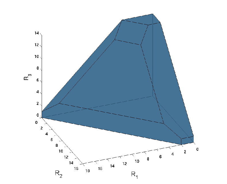
Figure 4 shows the capacity region for the case n1=18n_{1}=18,n2=16n_{2}=16,n3=14n_{3}=14,nM=6n_{M}=6 and nD=7n_{D}=7.

Refer to caption
Fig. 4: Capacity region of the system for n1=18n_{1}=18,n2=16n_{2}=16,n3=14n_{3}=14,nM=6n_{M}=6 and nD=7n_{D}=7.

V Conclusions

In this paper, we studied the linear deterministic model for a cellular-type channel where there are two users (in cell 1) transmitting to a receiver (base station 1), mutually interfering with a third transmitter (in cell 2) communicating with a second base station (base station 2). We studied the case of symmetric weak interference where the interference links from cell 1 user to the cell 2 base station are identical and the sum of the interference gains are less or equal then the smallest direct link. We derived the capacity region and the corresponding transmission scheme. Even though the system resembles the interference channel, the presence of the second link in cell 1 offers additional potential for aligning the interference caused by the two users at the receiver in the second cell. For this, the transmitted signals in cell 1 are chosen such that the interference at the second receiver aligns on the part of the signal that is unused by the transmitter in cell 2 as much as possible. Although we have considered a restricted setup in this paper, we believe that the achievability and converse arguments used in this paper give valuable insights for the consideration of more general systems.

Future work will study extensions to the more general case of more users and less restricted channel gains. Another interesting direction for further investigations are the connections to the Gaussian equivalent of the channel, specifically concerning approximate capacity characterizations and / or the determination of (generalized) degrees of freedom of the system.

References

  • [1] R. Etkin, D. Tse, and H. Wang, “Gaussian interference channel capacity to within one bit,” IEEE Trans. Inform. Theory, vol. 54, no. 12, pp. 5534–5562, Dec. 2008.
  • [2] S. Avestimehr, S. Diggavi, and D. Tse, “A deterministic approach to wireless relay networks,” in Proc. Allerton Conference on Communication, Control and Computing, Monticello, IL, USA, 2007.
  • [3] A. S. Avestimehr, S. N. Diggavi, and D. N. C. Tse, “Wireless network information flow: A deterministic approach,” IEEE Trans. Inform. Theory, vol. 57, no. 4, pp. 1872–1905, 2011.
  • [4] G. Bresler and D. Tse, “The two-user gaussian interference channel: a deterministic view,” European Trans. on Telecommunications, vol. 8, no. 4, pp. 333–354, 2008.
  • [5] V. Cadambe, S. Jafar, and S. Shamai, “Interference alignment on the deterministic channel and application to fully connected gaussian interference networks,” IEEE Trans. Inform. Theory, vol. 55, no. 1, pp. 269–274, 2009.
  • [6] C. Huang, V. Cadambe, and S. Jafar, “Interference alignment and the generalized degrees of freedom of the x channel,” in Proc. IEEE Int. Symp. Information Theory (ISIT), Seoul, Korea, June/July 2009, pp. 1929–1933.
  • [7] D. Tse and R. Yates, “Fading broadcast channels with state information at the receivers,” arXiv:0904.3165v1 [cs.IT], 2009.
  • [8] G. Bresler, A. Parekh, and D. Tse, “The approximate capacity of the many-to-one and one-to-many gaussian interference channels,” IEEE Trans. Inform. Theory, vol. 56, no. 9, pp. 4566–4592, 2010.
  • [9] V. Prabhakaran and P. Viswanath, “Interference channels with source cooperation,” IEEE Trans. Inform. Theory, vol. 57, no. 1, pp. 156–186, 2011.
  • [10] ——, “Interference channels with destination cooperation,” IEEE Trans. Inform. Theory, vol. 57, no. 1, pp. 187–209, 2011.
  • [11] B. Bandemer, A. El Gamal, and G. Vazquez-Vilar, “On the sum capacity of a class of cyclically symmetric deterministic interference channels,” in Proc. IEEE Int. Symp. Information Theory (ISIT), Seoul, Korea, June/July 2009, pp. 2622–2626.