跳到论文正文
W Papers独立论文阅读器 arXiv:1104.0118 论文正文 计算阅读时间 · 0%
引用这篇论文根据当前论文元数据生成,正式投稿前建议核对。


License: CC BY 3.0
arXiv:1104.0118v1 [cs.IT] 01 Apr 2011

A Comparative Study of Relaying Schemes with Decode-and-Forward over Nakagami-mm Fading Channels

George C. Alexandropoulos    Agisilaos Papadogiannis    Paschalis C. Sofotasios ††thanks: G. C. Alexandropoulos is with the Department of Telecommunications Science and Technology, University of Peloponnese, End of Karaiskaki Street, GR-22100 Tripolis, Greece (e-mail: alexandg@ieee.org).††thanks: A. Papadogiannis is with the Communications Research Group, Department of Electronics, University of York, York, YO10 5DD, United Kingdom (e-mail: ap851@ohm.york.ac.uk).††thanks: P. C. Sofotasios is with School of Electronic and Electrical Engineering, University of Leeds, Leeds, LS2 9JT, United Kingdom (e-mail: p.sofotasios@leeds.ac.uk).
Abstract

Utilizing relaying techniques to improve performance of wireless systems is a promising avenue. However, it is crucial to understand what type of relaying schemes should be used for achieving different performance objectives under realistic fading conditions. In this paper, we present a general framework for modelling and evaluating the performance of relaying schemes based on the decode-and-forward (DF) protocol over independent and not necessarily identically distributed (INID) Nakagami-mm fading channels. In particular, we present closed-form expressions for the statistics of the instantaneous output signal-to-noise ratio of four significant relaying schemes with DF; two based on repetitive transmission and the other two based on relay selection (RS). These expressions are then used to obtain closed-form expressions for the outage probability and the average symbol error probability for several modulations of all considered relaying schemes over INID Nakagami-mm fading. Importantly, it is shown that when the channel state information for RS is perfect, RS-based transmission schemes always outperform repetitive ones. Furthermore, when the direct link between the source and the destination nodes is sufficiently strong, relaying may not result in any gains and in this case it should be switched-off.

Index Terms: 
Bit error probability, cooperative diversity, Nakagami-mm fading, outage probability, relay selection, repetitive transmission.

I Introduction

The significance of multiple-input multiple-output (MIMO) techniques for modern wireless systems has been well appreciated. Multiple collocated antennas can improve transmission reliability and the achievable capacity through diversity, spatial multiplexing and/or interference suppression [1, 2]. However, the cost of mobile devices is proportional to their number of antennas and this creates a serious practical limitation for the use of MIMO. Cooperative diversity is a promising new avenue which allows cooperation amongst a number of wireless nodes which effectively profit from MIMO techniques without requiring multiple collocated antennas [3, 4].

Dual-hop cooperative diversity entails that the transmission of the source node towards a destination node is assisted by one or more relay nodes which can be seen to form a conceptual MIMO array [3]. Relay nodes can either be fixed, being part of the system infrastructure, or mobile, i.e., mobile nodes that relay signals intended for other mobile nodes [5]. Cooperative diversity is shown to improve the transmission reliability and the achievable capacity while it also extends coverage. Essentially, it can achieve diversity gains and has the additional advantage over conventional MIMO that the remote cooperating antennas experience very low or inexisting correlation [3, 6, 7, 8]. The performance of a system exploiting cooperative diversity depends on the employed relaying protocol and scheme, i.e., the way of utilizing relay nodes [3, 6, 7, 8]. Consequently, it is crucial to gain insights on which relay scheme is most suitable for achieving a particular objective; some common objectives are the minimization of the outage probability (OP) or the average symbol error probability (ASEP) [9, 10].

In the present work, we consider the decode-and-forward (DF) relaying protocol under the assumption that the message transmitted by the source is decoded and retransmitted to destination by one or more relays in a dual-hop fashion. We also take into account four relaying schemes; two based on repetitive transmission and the other two based on relay selection (RS). According to repetitive transmission, all relays that decode source’s message retransmit it repetitively to the destination node which employs diversity techniques to combine the different signal copies [11, 12]. One version of RS entails that amongst relays decoding the source’s message only one is selected to retransmit it to destination, the one with the strongest relay to destination channel [6, 13]. Another version of RS utilizes the best relay only in the case that it results in capacity gains over the direct source to destination transmission [7, 10]. In the literature such schemes have been considered partially and mainly assuming independent and identically distributed (IID) Rayleigh fading channels [11, 6, 13]. Recently, the Nakagami-mm fading model has received a lot of attention as it can describe more accurately the fading process and helps in understanding the gains of cooperative diversity [14, 9, 15, 16, 10, 17, 18]. However, there has not been a complete study that sheds light on the question of which relaying scheme is preferable and under which channel conditions.

In this paper, we present a general analytical framework for modeling and evaluating performance of relaying schemes with DF under independent and not necessarily identically distributed (INID) Nakagami-mm fading channels. Further to this, we obtain closed-form expressions for the OP and the ASEP performance of the RS and repetitive schemes when maximal ratio diversity (MRD) or selection diversity (SD) are employed at the destination node. We conclude that the RS-based transmission always performs better in terms of OP and ASEP than repetitive transmission when channel state information (CSI) for RS is perfect. In addition, when the direct source to destination link is sufficiently strong, relaying should be disabled when the objective is the minimization of OP. Although RS requires only two time slots for transmission (the repetitive scheme needs as many time slots as the number of decoding relays) its performance heavily relies on the quality of CSI for RS.

The remainder of this paper is structured as follows: Section II outlines the system and channel models. Section III presents closed-form expressions for the statistics of the instantaneous output SNR of the considered DF relaying schemes over INID Nakagami-mm fading channels. In Section IV, closed-from expressions are derived for the OP and ASEP performance of all relaying schemes. Section V contains numerical results and relevant discussion, whereas Section VI concludes the paper.

Notations: Throughout this paper, |𝔸|\left|\mathbb{A}\right| represents the cardinality of the set 𝔸\mathbb{A} and 𝔼​⟨⋅⟩{\mathbb{E}}\langle\cdot\rangle denotes the expectation operator. Pr⁡{⋅}\Pr\left\{\cdot\right\} denotes probability, 𝕃−1​{⋅;⋅}\mathbb{L}^{-1}\{\cdot;\cdot\} denotes the inverse Laplace transform and X∼𝒞​𝒩​(μ,σ2)X\sim\mathcal{C}\mathcal{N}\left(\mu,\sigma^{2}\right) represents a random variable (RV) following the complex normal distribution with mean μ\mu and variance σ2\sigma^{2}. Γ⁡(⋅)\Gamma\left(\cdot\right) is the Gamma function [19, eq. (8.310/1)] and Γ⁡(⋅,⋅)\mathsf{\Gamma}\left(\cdot,\cdot\right) is the lower incomplete Gamma function [19, eq. (8.350/1)]. Moreover, δ⁡(⋅)\delta\left(\cdot\right) is the Dirac function, u⁡(⋅)u\left(\cdot\right) is the unit step function and δ⁡(⋅,⋅)\delta\left(\cdot,\cdot\right) is the Kronecker Delta function.

II System and Channel Model

We consider a dual-hop cooperative wireless system, as illustrated in Fig. 1, consisting of L+2L+2 wireless nodes: one source node SS, a set 𝔸\mathbb{A} of LL relay nodes each denoted by RkR_{k}, k=1,2,…,Lk=1,2,\ldots,L, and one destination node DD. All RkR_{k}’s are assumed to operate in half-duplex mode, i.e., they cannot transmit and receive simultaneously, and node DD is assumed to possess perfectly S→DS\rightarrow D and all Rk→DR_{k}\rightarrow D CSI. We consider orthogonal DF (ODF) relaying [3] for which each RkR_{k} that successfully decodes SS’s signal retransmits it to DD; during each RkR_{k}’s transmission to DD node SS remains silent. Assuming repetitive transmission [3], L+1L+1 time slots are used to forward SS’s signal to DD in a predetermined order, whereas only two time slots are needed with RS-based transmission [6]. In particular, during the first time slot for both transmission strategies, SS broadcasts its signal to all RkR_{k}’s and also to DD. Considering quasi-static fading channels, the received signal at RkR_{k}’s and DD, respectively, during the first time slot can be mathematically expressed as

yD(1)=hS​D​s+nS​Dy_{D}^{(1)}=h_{SD}s+n_{SD} (1a)
yRk=hS​Rk​s+nS​Rky_{R_{k}}=h_{SR_{k}}s+n_{SR_{k}} (1b)

where hS​Dh_{SD} and hS​Rkh_{SR_{k}} denote the S→DS\rightarrow D and S→RkS\rightarrow R_{k}, respectively, complex-valued channel coefficients and ss is the transmitted complex message symbol with average symbol energy EsE_{s}. Moreover, the notations nS​Dn_{SD} and nS​Rkn_{SR_{k}} in (1) represent the additive white Gaussian noise (AWGN) of the S→DS\rightarrow D and S→RkS\rightarrow R_{k} channel, respectively, with nS​D,nS​Rk∼𝒞​𝒩​(0,N0)n_{SD},n_{SR_{k}}\sim\mathcal{C}\mathcal{N}\left(0,N_{0}\right). For both nS​Dn_{SD} and nS​Rkn_{SR_{k}}, it is assumed that they are statistically independent of ss.

Let us assume that set 𝔹⊆𝔸\mathbb{B}\subseteq\mathbb{A} contains the relay nodes that have successfully decoded SS’s signal during the first time slot of transmission. When repetitive transmission is utilized, LL more time slots are used for RkR_{k}’s belonging to 𝔹\mathbb{B} to forward ss to DD; each RkR_{k} retransmits ss during the kk-th time slot11 1 Note that the assignment of each time slot to RkR_{k}’s is performed in a predetermined order [3]. Thus, due to different Rk→DR_{k}\rightarrow D ∀k\forall\,k channel conditions and ODF relaying, there might be some unused time slots.. Hence, for quasi-static fading, the received signal at DD at the kk-th time slot can be expressed as

yD(k)=hRk​D​s+nRk​Dy_{D}^{(k)}=h_{R_{k}D}s+n_{R_{k}D} (2)

with hRk​Dh_{R_{k}D} representing the Rk→DR_{k}\rightarrow D complex-valued channel coefficient and nRk​D∼𝒞​𝒩​(0,N0)n_{R_{k}D}\sim\mathcal{C}\mathcal{N}\left(0,N_{0}\right) is AWGN of this channel that is assumed statistically independent of ss.

When RS-based transmission is used, one time slot is needed for the relay node RbestR_{\rm best} with the most favourable Rbest→DR_{\rm best}\rightarrow D channel conditions to forward SS’s signal to DD. Thus, for this transmission strategy and during the second time slot, the received signal at DD for quasi-static fading can be expressed as

yD(2)=hRbest​D​s+nRbest​Dy_{D}^{(2)}=h_{R_{\rm best}D}s+n_{R_{\rm best}D} (3)

where hRbest​Dh_{R_{\rm best}D} and nRbest​D∼𝒞​𝒩​(0,N0)n_{R_{\rm best}D}\sim\mathcal{C}\mathcal{N}\left(0,N_{0}\right) denote the Rk→DR_{k}\rightarrow D complex-valued channel coefficient and the AWGN for this channel, respectively. As (1) and (2), it is assumed that nRbest​Dn_{R_{\rm best}D} is statistically independent of ss.

The quasi-static fading channels hS​Dh_{SD}, hS​Rkh_{SR_{k}} and hRk​Dh_{R_{k}D} ∀k\forall\,k, and hRbest​Dh_{R_{\rm best}D} are assumed to be modeled as INID Nakagami-mm RVs [20]. Let γ0=|hS​D|2​Es/N0\gamma_{0}=\left|h_{SD}\right|^{2}E_{\text{s}}/N_{0} and γk=|hRk​D|2​Es/N0\gamma_{k}=\left|h_{R_{k}D}\right|^{2}E_{\text{s}}/N_{0}, k=1,2,…,Lk=1,2,\ldots,L, be the instantaneous received SNRs of the S→DS\rightarrow D and Rk→DR_{k}\rightarrow D link, respectively, with corresponding average values given by γ¯0=𝔼|⟨hS​D|2⟩Es/N0\overline{\gamma}_{0}=\mathbb{E}\left|\langle h_{SD}\right|^{2}\rangle E_{s}/N_{0} and γ¯k=𝔼⁡⟨|hRk​D|2⟩​Es/N0\overline{\gamma}_{k}=\mathbb{E}\langle\left|h_{R_{k}D}\right|^{2}\rangle E_{s}/N_{0}, respectively. Clearly, each γℓ\gamma_{\ell}, ℓ=0,1,…,L\ell=0,1,\ldots,L, is gamma distributed with probability density function (PDF) given by [21, Table 2.2]

fγℓ​(x)=CℓmℓΓ⁡(mℓ)​xmℓ−1​exp⁡(−Cℓ​x)f_{\gamma_{\ell}}\left(x\right)=\frac{C_{\ell}^{m_{\ell}}}{\Gamma\left(m_{\ell}\right)}x^{m_{\ell}-1}\exp\left(-C_{\ell}x\right) (4)

where mℓ≥1/2m_{\ell}\geq 1/2 denotes the Nakagami-mm fading parameter and Cℓ=mℓ/γ¯ℓC_{\ell}=m_{\ell}/\overline{\gamma}_{\ell}. Integrating (4), the cumulative distribution function (CDF) of each γℓ\gamma_{\ell} is easily obtained as

Fγℓ​(x)=Γ⁡(mℓ,Cℓ​x)Γ⁡(mℓ).F_{\gamma_{\ell}}\left(x\right)=\frac{\mathsf{\Gamma}\left(m_{\ell},C_{\ell}x\right)}{\Gamma\left(m_{\ell}\right)}. (5)

The PDFs and CDFs of the instantaneous received SNRs of the first hop, γL+k=|hS​Rk|2​Es/N0\gamma_{L+k}=\left|h_{SR_{k}}\right|^{2}E_{\text{s}}/N_{0} ∀k\forall\,k, are given using (4) and (5) by fγL+k​(x)f_{\gamma_{L+k}}\left(x\right) and FγL+k​(x)F_{\gamma_{L+k}}\left(x\right), respectively, with fading parameters and average SNRs denoted by mL+km_{L+k} and γ¯L+k=𝔼⁡⟨|hS​Rk|2⟩​Es/N0\overline{\gamma}_{L+k}=\mathbb{E}\langle\left|h_{SR_{k}}\right|^{2}\rangle E_{s}/N_{0}, respectively.

III Statistics of ODF Relaying Schemes

Relay station nodes that are able to decode the transmitted signal from SS constitute the decoding set 𝔹\mathbb{B}. Based on [3] and [13], for both transmission strategies the elements of 𝔹\mathbb{B} are obtained as

𝔹={Rk∈𝔸:log2⁡(1+γL+k)≥α​ℛ}\mathbb{B}=\left\{R_{k}\in\mathbb{A}:\log_{2}\left(1+\gamma_{L+k}\right)\geq\alpha\mathcal{R}\right\} (6)

where ℛ\mathcal{R} is SS’s transmit rate and α=L+1\alpha=L+1 for repetitive transmission, whereas α=2\alpha=2 for RS-based transmission. Hence, the probability that RkR_{k} does not belong to 𝔹\mathbb{B} is easily obtained as 𝒫k=Pr[γL+k<2α​ℛ−1]\mathcal{P}_{k}=\text{Pr}\left[\gamma_{L+k}<2^{\alpha\mathcal{R}}-1\right]. Substituting FγL+k​(x)F_{\gamma_{L+k}}\left(x\right) after using (5), a closed-form expression for 𝒫k\mathcal{P}_{k} in INID Nakagami-mm fading is given by

𝒫k=Γ⁡[mL+k,CL+k​(2α​ℛ−1)]Γ⁡(mL+k).\mathcal{P}_{k}=\frac{\mathsf{\Gamma}\left[m_{L+k},C_{L+k}\left(2^{\alpha\mathcal{R}}-1\right)\right]}{\Gamma\left(m_{L+k}\right)}. (7)

To analyze the performance of ODF relaying schemes, the S⟶DS\longrightarrow D direct channel plus the S⟶Rk⟶DS\longrightarrow R_{k}\longrightarrow D ∀k\forall\,k RS-assisted channels are effectively considered as L+1L+1 paths between SS and DD [11, 15]. In particular, let the zero-th path represent the S⟶DS\longrightarrow D direct link and the kk-th path the S⟶Rk⟶DS\longrightarrow R_{k}\longrightarrow D cascaded link. We define the instantaneous received SNRs at DD of these paths as g0g_{0} and gkg_{k}, respectively. By substituting (4) into [11, eq. (4)], the PDFs of gℓg_{\ell}’s, ℓ=0,1,…,L\ell=0,1,\ldots,L, are given by

fgℓ​(x)=𝒫ℓ​δ​(x)+(1−𝒫ℓ)​CℓmℓΓ⁡(mℓ)​xmℓ−1​exp⁡(−Cℓ​x)f_{g_{\ell}}\left(x\right)=\mathcal{P}_{\ell}\delta\left(x\right)+\frac{\left(1-\mathcal{P}_{\ell}\right)C_{\ell}^{m_{\ell}}}{\Gamma\left(m_{\ell}\right)}x^{m_{\ell}-1}\exp\left(-C_{\ell}x\right) (8)

where 𝒫0\mathcal{P}_{0} is the probability that DD belongs to 𝔹\mathbb{B}. Clearly, the direct S⟶DS\longrightarrow D path is not linked via a relay, i.e., 𝒫0=0\mathcal{P}_{0}=0, yielding fg0​(x)=fγ0​(x)f_{g_{0}}\left(x\right)=f_{\gamma_{0}}\left(x\right). Integrating (8) and using (5), yields the following expression for the CDF of the ℓ\ell-th cascaded path:

Fgℓ​(x)=𝒫ℓ​u​(x)+(1−𝒫ℓ)​Γ⁡(mℓ,Cℓ​x)Γ⁡(mℓ).F_{g_{\ell}}\left(x\right)=\mathcal{P}_{\ell}u\left(x\right)+\left(1-\mathcal{P}_{\ell}\right)\frac{\mathsf{\Gamma}\left(m_{\ell},C_{\ell}x\right)}{\Gamma\left(m_{\ell}\right)}. (9)

Note again that for the direct S⟶DS\longrightarrow D path yields Fg0​(x)=Fγ0​(x)F_{g_{0}}\left(x\right)=F_{\gamma_{0}}\left(x\right).

III-A Repetitive Transmission

The incoming signals at DD from SS and Rk∈𝔹R_{k}\in\mathbb{B} ∀k\forall\,k may be combined using a time-diversity version of MRD [3] and SD [12]. In particular, DD combines SS’s signal received at time slot one with the SS’s replicas received from all Rk∈𝔹R_{k}\in\mathbb{B} ∀k\forall\,k at the LL subsequent slots using either the rules of MRD or SD.

III-A1 Repetitive with MRD

With MRD the instantaneous SNR at DD’s output is expressed as

gend=g0+∑i=1|𝔹|gi.g_{\text{end}}=g_{0}+\sum_{i=1}^{\left|\mathbb{B}\right|}g_{i}. (10)

Since gℓg_{\ell}’s, ℓ=0,1,…,L\ell=0,1,\ldots,L, are independent, the moment generating function (MGF) of gendg_{\text{end}} can be easily obtained as the product of the MGFs of gℓg_{\ell}’s. As shown in [15] for INID Nakagami-mm fading, using (8) and the definition of the MGF of gkg_{k}, k=1,2,…,Lk=1,2,\ldots,L,

Mgk​(s)=∫0∞exp⁡(−s​x)​fgk​(x)​𝑑x,M_{g_{k}}\left(s\right)=\int_{0}^{\infty}\exp\left(-sx\right)f_{g_{k}}\left(x\right)dx, (11)

yields ℳgk​(s)=𝒫k+(1−𝒫k)​Ckmk​(s+Ck)−mk\mathcal{M}_{g_{k}}\left(s\right)=\mathcal{P}_{k}+\left(1-\mathcal{P}_{k}\right)C_{k}^{m_{k}}\left(s+C_{k}\right)^{-m_{k}}. Similarly, using (4) the MGF of g0g_{0} is easily obtained as ℳg0​(s)=C0m0​(s+C0)−m0\mathcal{M}_{g_{0}}\left(s\right)=C_{0}^{m_{0}}\left(s+C_{0}\right)^{-m_{0}}. Hence, the following closed-form expression for the MGF of gendg_{\text{end}} in INID Nakagami-mm is deduced

ℳgend​(s)=C0m0​(s+C0)−m0​∏k=1L[𝒫k+(1−𝒫k)​Ckmk​(s+Ck)−mk].\mathcal{M}_{g_{\text{end}}}\left(s\right)=C_{0}^{m_{0}}\left(s+C_{0}\right)^{-m_{0}}\prod_{k=1}^{L}\left[\mathcal{P}_{k}+\left(1-\mathcal{P}_{k}\right)C_{k}^{m_{k}}\left(s+C_{k}\right)^{-m_{k}}\right]. (12)

Using the MGF-based approach [21], the CDF of gendg_{\text{end}} can be obtained as

Fgend​(x)=𝕃−1​{ℳgend​(s)s;x}.F_{g_{\text{end}}}\left(x\right)=\mathbb{L}^{-1}\left\{\frac{\mathcal{M}_{g_{\text{end}}}\left(s\right)}{s};x\right\}. (13)

Substituting (12) in (13) and similar to the analysis presented in [15], a closed-form expression for Fgend​(x)F_{g_{\text{end}}}\left(x\right) of repetitive transmission with MRD over INID Nakagami-mm with integer mℓm_{\ell}’s and distinct CℓC_{\ell}’s is given by

Fgend​(x)=(∏ℓ=0L𝒫ℓ){1+∑{λk}k=0L(∏n=0k1−𝒫λn𝒫λnCλnmλn)×∑p=0k∑q=1mλpψpCλpq[1−exp(−Cλpx)∑ℓ=0q−1(Cλp​x)ℓℓ!]}\begin{split}F_{g_{\text{end}}}\left(x\right)=&\left(\prod_{\ell=0}^{L}\mathcal{P}_{\ell}\right)\left\{1+\sum_{\left\{\lambda_{k}\right\}_{k=0}^{L}}\left(\prod_{n=0}^{k}\frac{1-\mathcal{P}_{\lambda_{n}}}{\mathcal{P}_{\lambda_{n}}}C_{\lambda_{n}}^{m_{\lambda_{n}}}\right)\right.\\ &\left.\times\sum_{p=0}^{k}\sum_{q=1}^{m_{\lambda_{p}}}\frac{\psi_{p}}{C_{\lambda_{p}}^{q}}\left[1-\exp\left(-C_{\lambda_{p}}x\right)\sum_{\ell=0}^{q-1}\frac{\left(C_{\lambda_{p}}x\right)^{\ell}}{\ell!}\right]\right\}\end{split} (14)

The symbol ∑{αi}i=κI\sum_{\left\{\alpha_{i}\right\}_{i=\kappa}^{I}} is used for short-hand representation of multiple summations ∑i=κI\sum_{i=\kappa}^{I} ∑ακ=κI−i+κ\sum_{\alpha_{\kappa}=\kappa}^{I-i+\kappa} ∑ακ+1=ακ+1I−i+κ+1\sum_{\alpha_{\kappa+1}=\alpha_{\kappa}+1}^{I-i+\kappa+1} ⋯\cdots ∑αi=αi−1+1I\sum_{\alpha_{i}=\alpha_{i-1}+1}^{I} and ψp=Ψp​(s)(mλp−q)|s=−Cλp/(mλp−q)!\psi_{p}=\Psi_{p}\left(s\right)^{(m_{\lambda_{p}}-q)}|_{s=-C_{\lambda_{p}}}/(m_{\lambda_{p}}-q)! with Ψp​(s)=(s+Cλp)mλp​∏n=0k(s+Cλn)−mλn\Psi_{p}\left(s\right)=(s+C_{\lambda_{p}})^{m_{\lambda_{p}}}\prod_{n=0}^{k}(s+C_{\lambda_{n}})^{-m_{\lambda_{n}}}. For Cℓ=CC_{\ell}=C ∀ℓ\forall\,\ell with arbitrary values for mℓm_{\ell}’s and following a similar analysis as for the derivation of (14), a closed-form expression for Fgend​(x)F_{g_{\text{end}}}\left(x\right) can be obtained as

Fgend​(x)=(∏ℓ=0L𝒫ℓ)​{1+∑{λk}k=0L(∏n=0k1−𝒫λn𝒫λn)​Γ​(∑n=0kmλn,C​x)/Γ⁡(∑n=0kmλn)}.F_{g_{\text{end}}}\left(x\right)=\left(\prod_{\ell=0}^{L}\mathcal{P}_{\ell}\right)\left\{1+\sum_{\left\{\lambda_{k}\right\}_{k=0}^{L}}\left(\prod_{n=0}^{k}\frac{1-\mathcal{P}_{\lambda_{n}}}{\mathcal{P}_{\lambda_{n}}}\right)\mathsf{\Gamma}\left(\sum_{n=0}^{k}m_{\lambda_{n}},Cx\right)/\Gamma\left(\sum_{n=0}^{k}m_{\lambda_{n}}\right)\right\}. (15)

III-A2 Repetitive with SD

Alternatively to MRD, DD may use a time-diversity version of SD to combine the signals from SS and Rk∈𝔹R_{k}\in\mathbb{B} ∀k\forall\,k [12]. With this diversity technique the instantaneous SNR at DD’s output is given by

gend=maxRk∈ℂ⁡gkg_{\text{end}}=\max_{R_{k}\in\mathbb{C}}g_{k} (16)

where ℂ={S}∪𝔹\mathbb{C}=\{S\}\cup\mathbb{B}. The gℓg_{\ell}’s, ℓ=0,1,…,L\ell=0,1,\ldots,L, are assumed independent, therefore Fgend​(x)F_{g_{\text{end}}}\left(x\right) of (16) can be easily obtained as the product of the CDFs of gℓg_{\ell}’s. Substituting (5) and (9) for g0g_{0} and gkg_{k} ∀k=1,2,…,L\forall\,k=1,2,\ldots,L, respectively, a closed-form expression for Fgend​(x)F_{g_{\text{end}}}\left(x\right) of repetitive transmission with SD over INID Nakagami-mm fading can be derived as

Fgend​(x)=Fγ0​(x)​Fgbest​(x)F_{g_{\text{end}}}\left(x\right)=F_{\gamma_{0}}\left(x\right)F_{g_{\text{best}}}\left(x\right) (17)

where Fgbest​(x)F_{g_{\text{best}}}\left(x\right) is the CDF of the instantaneous SNR of the Rbest→DR_{\rm best}\rightarrow D channel, i.e., of

gbest=maxRk∈𝔹⁡gk,g_{\text{best}}=\max_{R_{k}\in\mathbb{B}}g_{k}, (18)

which is easily obtained using (9) for INID Nakagami-mm fading as

Fgbest​(x)=∏k=1L[𝒫k​u​(x)+(1−𝒫k)​Γ⁡(mk,Ck​x)Γ⁡(mk)].F_{g_{\text{best}}}\left(x\right)=\prod_{k=1}^{L}\left[\mathcal{P}_{k}u\left(x\right)+\left(1-\mathcal{P}_{k}\right)\frac{\mathsf{\Gamma}\left(m_{k},C_{k}x\right)}{\Gamma\left(m_{k}\right)}\right]. (19)

Differentiating (17), the PDF of gendg_{\text{end}} is given by

fgend​(x)=fγ0​(x)​Fgbest​(x)+Fγ0​(x)​fgbest​(x)f_{g_{\text{end}}}\left(x\right)=f_{\gamma_{0}}\left(x\right)F_{g_{\text{best}}}\left(x\right)+F_{\gamma_{0}}\left(x\right)f_{g_{\text{best}}}\left(x\right) (20)

where fgbest​(x)f_{g_{\text{best}}}\left(x\right) is the PDF of gbestg_{\text{best}}. To obtain an expression for fgbest​(x)f_{g_{\text{best}}}\left(x\right), we first use [19, eq. (8.352/1)] to obtain (19) for integer mℓm_{\ell}’s yielding

Fgbest​(x)=∏k=1L{𝒫k​u​(x)+(1−𝒫k)​[1−exp⁡(−Ck​x)​∑i=0mk−1(Ck​x)ii!]}.F_{g_{\text{best}}}\left(x\right)=\prod_{k=1}^{L}\left\{\mathcal{P}_{k}u\left(x\right)+\left(1-\mathcal{P}_{k}\right)\left[1-\exp\left(-C_{k}x\right)\sum_{i=0}^{m_{k}-1}\frac{\left(C_{k}x\right)^{i}}{i!}\right]\right\}. (21)

Then, differentiating (21) and using the formula

∏i=κI(χi+ψi)=∏i=κIχi+∑{αi}i=κI∏s=κiψαs​∏t=κt≠{αu}u=κiIχt,\prod_{i=\kappa}^{I}\left(\chi_{i}+\psi_{i}\right)=\prod_{i=\kappa}^{I}\chi_{i}+\sum_{\left\{\alpha_{i}\right\}_{i=\kappa}^{I}}\prod_{s=\kappa}^{i}\psi_{\alpha_{s}}\prod_{\begin{subarray}{c}t=\kappa\\ t\neq\left\{\alpha_{u}\right\}_{u=\kappa}^{i}\end{subarray}}^{I}\chi_{t}, (22)

where symbol ∑{αi}i=κI\sum_{\left\{\alpha_{i}\right\}_{i=\kappa}^{I}} is used for short-hand representation of multiple summations ∑i=κI\sum_{i=\kappa}^{I} ∑ακ=κI−i+κ∑ακ+1=ακ+1I−i+κ+1⋯∑αi=αi−1+1I\sum_{\alpha_{\kappa}=\kappa}^{I-i+\kappa}\sum_{\alpha_{\kappa+1}=\alpha_{\kappa}+1}^{I-i+\kappa+1}\cdots\sum_{\alpha_{i}=\alpha_{i-1}+1}^{I}, we obtain after some algebraic manipulations the following closed-form expression for fgbest​(x)f_{g_{\text{best}}}\left(x\right) in INID Nakagami-mm fading with integer mℓm_{\ell}’s:

fgbest(x)=(∏k=1L𝒫k){δ(x)+∑{λk}k=1L∑{μj}j=1k(−1)j(∏n=1k1−𝒫λn𝒫λn)×[−(∑p=1jCλμp)exp(−x∑p=1jCλμp)+∑{νi}i=1j(∑s=1piνs)(∏s=1p∑iνs=1mλμνs−1Cλμνsiνsiνs!)×x∑s=1piνs−1exp(−xξp,j)(1−ξp,j​x∑s=1piνs)]}.\begin{split}&f_{g_{\text{best}}}\left(x\right)=\left(\prod_{k=1}^{L}\mathcal{P}_{k}\right)\left\{\delta\left(x\right)+\sum_{\left\{\lambda_{k}\right\}_{k=1}^{L}}\sum_{\left\{\mu_{j}\right\}_{j=1}^{k}}\left(-1\right)^{j}\left(\prod_{n=1}^{k}\frac{1-\mathcal{P}_{\lambda_{n}}}{\mathcal{P}_{\lambda_{n}}}\right)\right.\\ &\left.\times\left[-\left(\sum_{p=1}^{j}C_{\lambda_{\mu_{p}}}\right)\exp\left(-x\sum_{p=1}^{j}C_{\lambda_{\mu_{p}}}\right)+\sum_{\left\{\nu_{i}\right\}_{i=1}^{j}}\left(\sum_{s=1}^{p}i_{\nu_{s}}\right)\left(\prod_{s=1}^{p}\sum_{i_{\nu_{s}}=1}^{m_{\lambda_{\mu_{\nu_{s}}}}-1}\frac{C_{\lambda_{\mu_{\nu_{s}}}}^{i_{\nu_{s}}}}{i_{\nu_{s}}!}\right)\right.\right.\\ &\left.\left.\times x^{\sum_{s=1}^{p}i_{\nu_{s}}-1}\exp\left(-x\xi_{p,j}\right)\left(1-\frac{\xi_{p,j}x}{\sum_{s=1}^{p}i_{\nu_{s}}}\right)\right]\right\}.\end{split} (23)

In (23), parameters ξp,j\xi_{p,j}’s, with pp and jj being positive integers, are given by

ξp,j=∑s=1pCλμνs+∑t=1t≠{νu}u=1pjCλμt.\xi_{p,j}=\sum_{s=1}^{p}C_{\lambda_{\mu_{\nu_{s}}}}+\sum_{\begin{subarray}{c}t=1\\ t\neq\left\{\nu_{u}\right\}_{u=1}^{p}\end{subarray}}^{j}C_{\lambda_{\mu_{t}}}. (24)

Substituting (4) and (5) for integer mℓm_{\ell}’s, i.e., after using [19, eq. (8.352/1)] for expressing Γ⁡(⋅,⋅)\mathsf{\Gamma}\left(\cdot,\cdot\right)’s, as well as (21) and (23) to (20), a closed-form expression for fgend​(x)f_{g_{\text{end}}}\left(x\right) over INID Nakagami-mm fading with integer values of mℓm_{\ell}’s and distinct CℓC_{\ell}’s can be obtained after some algebraic manipulations as

fgend(x)=(∏k=1L𝒫k){C0m0Γ⁡(m0)xm0−1exp(−C0x){u(x)+∑{λk}k=1L∑{μj}j=1k(−1)j×(∏n=1k1−𝒫λn𝒫λn)[exp(−x∑p=1jCλμp)−1+∑{νi}i=1j(∏s=1p∑iνs=1mλμνs−1Cλμνsiνsiνs!)×x∑s=1piνsexp(−xξp,j)]}+[1−exp(−C0x)∑i=0m0−1(C0​x)ii!]×{δ(x)+∑{λk}k=1L∑{μj}j=1k(−1)j(∏n=1k1−𝒫λn𝒫λn)×[−(∑p=1jCλμp)exp(−x∑p=1jCλμp)+∑{νi}i=1j(∑s=1piνs)(∏s=1p∑iνs=1mλμνs−1Cλμνsiνsiνs!)×x∑s=1piνs−1exp(−xξp,j)(1−ξp,j​x∑s=1piνs)]}}.\begin{split}&f_{g_{\text{end}}}\left(x\right)=\left(\prod_{k=1}^{L}\mathcal{P}_{k}\right)\left\{\frac{C_{0}^{m_{0}}}{\Gamma\left(m_{0}\right)}x^{m_{0}-1}\exp\left(-C_{0}x\right)\left\{u\left(x\right)+\sum_{\left\{\lambda_{k}\right\}_{k=1}^{L}}\sum_{\left\{\mu_{j}\right\}_{j=1}^{k}}\left(-1\right)^{j}\right.\right.\\ &\left.\left.\times\left(\prod_{n=1}^{k}\frac{1-\mathcal{P}_{\lambda_{n}}}{\mathcal{P}_{\lambda_{n}}}\right)\left[\exp\left(-x\sum_{p=1}^{j}C_{\lambda_{\mu_{p}}}\right)-1+\sum_{\left\{\nu_{i}\right\}_{i=1}^{j}}\left(\prod_{s=1}^{p}\sum_{i_{\nu_{s}}=1}^{m_{\lambda_{\mu_{\nu_{s}}}}-1}\frac{C_{\lambda_{\mu_{\nu_{s}}}}^{i_{\nu_{s}}}}{i_{\nu_{s}}!}\right)\right.\right.\right.\\ &\left.\left.\left.\times x^{\sum_{s=1}^{p}i_{\nu_{s}}}\exp\left(-x\xi_{p,j}\right)\right]\right\}+\left[1-\exp\left(-C_{0}x\right)\sum_{i=0}^{m_{0}-1}\frac{\left(C_{0}x\right)^{i}}{i!}\right]\right.\\ &\left.\times\left\{\delta\left(x\right)+\sum_{\left\{\lambda_{k}\right\}_{k=1}^{L}}\sum_{\left\{\mu_{j}\right\}_{j=1}^{k}}\left(-1\right)^{j}\left(\prod_{n=1}^{k}\frac{1-\mathcal{P}_{\lambda_{n}}}{\mathcal{P}_{\lambda_{n}}}\right)\right.\right.\\ &\left.\left.\times\left[-\left(\sum_{p=1}^{j}C_{\lambda_{\mu_{p}}}\right)\exp\left(-x\sum_{p=1}^{j}C_{\lambda_{\mu_{p}}}\right)+\sum_{\left\{\nu_{i}\right\}_{i=1}^{j}}\left(\sum_{s=1}^{p}i_{\nu_{s}}\right)\left(\prod_{s=1}^{p}\sum_{i_{\nu_{s}}=1}^{m_{\lambda_{\mu_{\nu_{s}}}}-1}\frac{C_{\lambda_{\mu_{\nu_{s}}}}^{i_{\nu_{s}}}}{i_{\nu_{s}}!}\right)\right.\right.\right.\\ &\left.\left.\left.\times x^{\sum_{s=1}^{p}i_{\nu_{s}}-1}\exp\left(-x\xi_{p,j}\right)\left(1-\frac{\xi_{p,j}x}{\sum_{s=1}^{p}i_{\nu_{s}}}\right)\right]\right\}\right\}.\end{split} (25)

To obtain the MGF of gendg_{\text{end}}, we substitute the fgend​(x)f_{g_{\text{end}}}\left(x\right) expression given by (25) to the definition of the MGF given by (11), i.e., after replacing gkg_{k} with gendg_{\text{end}} in (11), and use[19, eq. (3.381/4)] to solve the resulting integrals. In particular, by first deriving using (23) the following closed-form expression for the MGF of gbestg_{\text{best}} in INID Nakagami-mm fading with integer values of mℓm_{\ell}’s and distinct CℓC_{\ell}’s:

Mgbest(s)=(∏k=1L𝒫k){1+∑{λk}k=1L∑{μj}j=1k(−1)j(∏n=1k1−𝒫λn𝒫λn)×{−(∑p=1jCλμp)(s+∑p=1jCλμp)−1+∑{νi}i=1j(∑s=1piνs)!(∏s=1p∑iνs=1mλμνs−1Cλμνsiνsiνs!)×(s+ξp,j)−∑s=1piνs[1−ξp,j(s+ξp,j)−1]}},\begin{split}&M_{g_{\text{best}}}\left(s\right)=\left(\prod_{k=1}^{L}\mathcal{P}_{k}\right)\left\{1+\sum_{\left\{\lambda_{k}\right\}_{k=1}^{L}}\sum_{\left\{\mu_{j}\right\}_{j=1}^{k}}\left(-1\right)^{j}\left(\prod_{n=1}^{k}\frac{1-\mathcal{P}_{\lambda_{n}}}{\mathcal{P}_{\lambda_{n}}}\right)\right.\\ &\times\left.\left\{-\left(\sum_{p=1}^{j}C_{\lambda_{\mu_{p}}}\right)\left(s+\sum_{p=1}^{j}C_{\lambda_{\mu_{p}}}\right)^{-1}+\sum_{\left\{\nu_{i}\right\}_{i=1}^{j}}\left(\sum_{s=1}^{p}i_{\nu_{s}}\right)!\left(\prod_{s=1}^{p}\sum_{i_{\nu_{s}}=1}^{m_{\lambda_{\mu_{\nu_{s}}}}-1}\frac{C_{\lambda_{\mu_{\nu_{s}}}}^{i_{\nu_{s}}}}{i_{\nu_{s}}!}\right)\right.\right.\\ &\left.\left.\times\left(s+\xi_{p,j}\right)^{-\sum_{s=1}^{p}i_{\nu_{s}}}\left[1-\xi_{p,j}\left(s+\xi_{p,j}\right)^{-1}\right]\right\}\right\},\end{split} (26)

a closed-form expression for the MGF of gendg_{\text{end}} of repetitive transmission with SD over INID Nakagami-mm fading channels with integer values of mℓm_{\ell}’s and distinct CℓC_{\ell}’s is given by

ℳgend(s)=(∏k=1L𝒫k){C0m0{(s+C0)−m0+∑{λk}k=1L∑{μj}j=1k(−1)j(∏n=1k1−𝒫λn𝒫λn)×[(s+C0+∑p=1jCλμp)−m0−(s+C0)−m0+∑{νi}i=1j(∏s=1p∑iνs=1mλμνs−1Cλμνsiνsiνs!)×(m0+∑s=1piνs−1)!(m0−1)!(s+C0+ξp,j)−(m0+∑s=1piνs)]}+{∑{λk}k=1L∑{μj}j=1k(−1)j(∏n=1k1−𝒫λn𝒫λn){(∑p=1jCλμp)∑q=0m0−1C0q(s+C0+∑p=1jCλμp)−(q+1)+∑{νi}i=1j(∑s=1piνs)(∏s=1p∑iνs=1mλμνs−1Cλμνsiνsiνs!)∑q=0m0−1C0qq!(s+C0+ξp,j)−(q+∑s=1piνs+1)×(q+∑s=1piνs−1)![qξp,j−(s+C0)∑s=1piνs]}}}+Mgbest(s).\begin{split}&\mathcal{M}_{g_{\text{end}}}\left(s\right)=\left(\prod_{k=1}^{L}\mathcal{P}_{k}\right)\left\{C_{0}^{m_{0}}\left\{\left(s+C_{0}\right)^{-m_{0}}+\sum_{\left\{\lambda_{k}\right\}_{k=1}^{L}}\sum_{\left\{\mu_{j}\right\}_{j=1}^{k}}\left(-1\right)^{j}\left(\prod_{n=1}^{k}\frac{1-\mathcal{P}_{\lambda_{n}}}{\mathcal{P}_{\lambda_{n}}}\right)\right.\right.\\ &\left.\left.\times\left[\left(s+C_{0}+\sum_{p=1}^{j}C_{\lambda_{\mu_{p}}}\right)^{-m_{0}}-\left(s+C_{0}\right)^{-m_{0}}+\sum_{\left\{\nu_{i}\right\}_{i=1}^{j}}\left(\prod_{s=1}^{p}\sum_{i_{\nu_{s}}=1}^{m_{\lambda_{\mu_{\nu_{s}}}}-1}\frac{C_{\lambda_{\mu_{\nu_{s}}}}^{i_{\nu_{s}}}}{i_{\nu_{s}}!}\right)\right.\right.\right.\\ &\left.\left.\left.\times\frac{\left(m_{0}+\sum_{s=1}^{p}i_{\nu_{s}}-1\right)!}{\left(m_{0}-1\right)!}\left(s+C_{0}+\xi_{p,j}\right)^{-\left(m_{0}+\sum_{s=1}^{p}i_{\nu_{s}}\right)}\right]\right\}+\left\{\sum_{\left\{\lambda_{k}\right\}_{k=1}^{L}}\sum_{\left\{\mu_{j}\right\}_{j=1}^{k}}\left(-1\right)^{j}\right.\right.\\ &\left.\left.\left(\prod_{n=1}^{k}\frac{1-\mathcal{P}_{\lambda_{n}}}{\mathcal{P}_{\lambda_{n}}}\right)\left\{\left(\sum_{p=1}^{j}C_{\lambda_{\mu_{p}}}\right)\sum_{q=0}^{m_{0}-1}C_{0}^{q}\left(s+C_{0}+\sum_{p=1}^{j}C_{\lambda_{\mu_{p}}}\right)^{-(q+1)}\right.\right.\right.\\ &\left.\left.\left.+\sum_{\left\{\nu_{i}\right\}_{i=1}^{j}}\left(\sum_{s=1}^{p}i_{\nu_{s}}\right)\left(\prod_{s=1}^{p}\sum_{i_{\nu_{s}}=1}^{m_{\lambda_{\mu_{\nu_{s}}}}-1}\frac{C_{\lambda_{\mu_{\nu_{s}}}}^{i_{\nu_{s}}}}{i_{\nu_{s}}!}\right)\sum_{q=0}^{m_{0}-1}\frac{C_{0}^{q}}{q!}\left(s+C_{0}+\xi_{p,j}\right)^{-\left(q+\sum_{s=1}^{p}i_{\nu_{s}}+1\right)}\right.\right.\right.\\ &\left.\left.\left.\times\left(q+\sum_{s=1}^{p}i_{\nu_{s}}-1\right)!\left[q\xi_{p,j}-\left(s+C_{0}\right)\sum_{s=1}^{p}i_{\nu_{s}}\right]\right\}\right\}\right\}+M_{g_{\text{best}}}\left(s\right).\end{split} (27)

For equal CℓC_{\ell}’s, i.e., IID Nakagami-mm fading with mℓ=mm_{\ell}=m and γ¯ℓ=γ¯\overline{\gamma}_{\ell}=\overline{\gamma} ∀ℓ\forall\,\ell, following a similar procedure as for the derivation of (27) and using the binomial and multinomial theorems [19, eq. (1.111)], we first obtain the following closed-form expression for Mgbest​(s)M_{g_{\text{best}}}\left(s\right) for integer mm

Mgbest(s)=L𝒫L{1/L+(1−𝒫)Cm(s+C)−m+∑k=1L−1(L−1k)(1−𝒫)k𝒫k+1×{𝒫+(1−𝒫)Cm(s+C)−m+∑j=1k(kj)(−1)j×[𝒫+∑n1+n2+⋯+nm=jj(1−𝒫)​Cm+σ∏j=2m−1(j!)nj+1∏i=1mni−1(m−1)![s+(j+1)C]−(m+σ)]}}\begin{split}&M_{g_{\text{best}}}\left(s\right)=L\mathcal{P}^{L}\left\{1/L+\left(1-\mathcal{P}\right)C^{m}\left(s+C\right)^{-m}+\sum_{k=1}^{L-1}\binom{L-1}{k}\frac{\left(1-\mathcal{P}\right)^{k}}{\mathcal{P}^{k+1}}\right.\\ &\left.\times\left\{\mathcal{P}+\left(1-\mathcal{P}\right)C^{m}\left(s+C\right)^{-m}+\sum_{j=1}^{k}\binom{k}{j}\left(-1\right)^{j}\right.\right.\\ &\left.\left.\times\left[\mathcal{P}+\sum_{n_{1}+n_{2}+\cdots+n_{m}=j}^{j}\frac{\left(1-\mathcal{P}\right)C^{m+\sigma}}{\prod_{j=2}^{m-1}\left(j!\right)^{n_{j+1}}}\frac{\prod_{i=1}^{m}n_{i}^{-1}}{\left(m-1\right)!}\left[s+(j+1)C\right]^{-\left(m+\sigma\right)}\right]\right\}\right\}\end{split} (28)

where C=m/γ¯C=m/\overline{\gamma}, 𝒫=𝒫k\mathcal{P}=\mathcal{P}_{k} ∀k\forall\,k, σ=∑i=2m(i−1)​ni\sigma=\sum_{i=2}^{m}(i-1)n_{i} and symbol ∑n1+n2+⋯+nm=jj\sum_{n_{1}+n_{2}+\cdots+n_{m}=j}^{j} is used for short-hand representation of multiple summations ∑n1=0j∑n2=0j⋯∑nm=0jδ(∑i=1mni,j)\sum_{n_{1}=0}^{j}\sum_{n_{2}=0}^{j}\cdots\sum_{n_{m}=0}^{j}\delta(\sum_{i=1}^{m}n_{i},j). Using (20) for IID Nakagami-mm fading, (28) and after some algebraic manipulations, a closed-form expression for Mgend​(s)M_{g_{\text{end}}}\left(s\right) of repetitive transmission with SD in IID Nakagami-mm fading channels with integer mm is obtained as

Mgend(s)=L𝒫L{Cm{[1/L+(1−𝒫)](s+C)−m−(1−𝒫)B0,1(s)+∑k=1L−1(L−1k)×(1−𝒫)k𝒫k+1{[𝒫+(1−𝒫)](s+C)−m−(1−𝒫)B0,1(s)+∑j=1k(kj)(−1)j[𝒫×(s+C)−m+∑n1+n2+⋯+nm=jj(1−𝒫)∏j=2m−1(j!)nj+1∏i=1mni−1(m−1)!{(s+C)−m−Bσ,j+1(s)}]}}−Cm{(1−𝒫)B0,1(s)+∑k=1L−1(L−1k)(1−𝒫)k𝒫k+1{(1−𝒫)B0,1(s)+∑j=1k(kj)(−1)j×∑n1+n2+⋯+nm=jj(1−𝒫)​Cσ∏j=2m−1(j!)nj+1​∏i=1mni−1(m−1)!​∑q=0m−1Cqq!​(m+σ−1)!​(m+q+σ−1)!×[s+(λ+1)C]−(m+q)}}}+Mgbest(s)\begin{split}&M_{g_{\text{end}}}\left(s\right)=L\mathcal{P}^{L}\left\{C^{m}\left\{\left[1/L+\left(1-\mathcal{P}\right)\right]\left(s+C\right)^{-m}-(1-\mathcal{P})B_{0,1}\left(s\right)+\sum_{k=1}^{L-1}\binom{L-1}{k}\right.\right.\\ &\left.\left.\times\frac{\left(1-\mathcal{P}\right)^{k}}{\mathcal{P}^{k+1}}\left\{\left[\mathcal{P}+\left(1-\mathcal{P}\right)\right]\left(s+C\right)^{-m}-(1-\mathcal{P})B_{0,1}\left(s\right)+\sum_{j=1}^{k}\binom{k}{j}\left(-1\right)^{j}\left[\mathcal{P}\right.\right.\right.\right.\\ &\left.\left.\left.\left.\times\left(s+C\right)^{-m}+\sum_{n_{1}+n_{2}+\cdots+n_{m}=j}^{j}\frac{\left(1-\mathcal{P}\right)}{\prod_{j=2}^{m-1}\left(j!\right)^{n_{j+1}}}\frac{\prod_{i=1}^{m}n_{i}^{-1}}{\left(m-1\right)!}\left\{\left(s+C\right)^{-m}-B_{\sigma,j+1}\left(s\right)\right\}\right]\right\}\right\}\right.\\ &\left.-C^{m}\left\{\left(1-\mathcal{P}\right)B_{0,1}\left(s\right)+\sum_{k=1}^{L-1}\binom{L-1}{k}\frac{\left(1-\mathcal{P}\right)^{k}}{\mathcal{P}^{k+1}}\left\{\left(1-\mathcal{P}\right)B_{0,1}\left(s\right)+\sum_{j=1}^{k}\binom{k}{j}\left(-1\right)^{j}\right.\right.\right.\\ &\left.\left.\left.\times\sum_{n_{1}+n_{2}+\cdots+n_{m}=j}^{j}\frac{\left(1-\mathcal{P}\right)C^{\sigma}}{\prod_{j=2}^{m-1}\left(j!\right)^{n_{j+1}}}\frac{\prod_{i=1}^{m}n_{i}^{-1}}{\left(m-1\right)!}\sum_{q=0}^{m-1}\frac{C^{q}}{q!(m+\sigma-1)!}(m+q+\sigma-1)!\right.\right.\right.\\ &\left.\left.\left.\times[s+(\lambda+1)C]^{-(m+q)}\right\}\right\}\right\}+M_{g_{\text{best}}}\left(s\right)\end{split} (29)

where function Bκ,λ​(s)B_{\kappa,\lambda}\left(s\right), with κ\kappa and λ\lambda being positive integers, is given by

Bκ,λ​(s)=∑q=0m+κ−1(λ​C)qq!​(m−1)!​(m+q−1)!​[s+(λ+1)​C]−(m+q).B_{\kappa,\lambda}\left(s\right)=\sum_{q=0}^{m+\kappa-1}\frac{(\lambda C)^{q}}{q!(m-1)!}(m+q-1)![s+(\lambda+1)C]^{-(m+q)}. (30)

III-B RS-based Transmission

When RS-based transmission is utilized, RS [6] is first performed to obtain RbestR_{\rm best}. Relay node RbestR_{\rm best} is the one experiencing the most favorable Rk→DR_{k}\rightarrow D ∀k\forall\,k channel conditions, i.e., its instantaneous SNR is given by (18). Using expressions derived in Section III-A, we next obtain closed-form expressions for the statistics of a pure RS scheme [13, 10] that combines at DD the signals from SS and RbestR_{\rm best} using a time-diversity version of MRD as well as of a rate-selective one [10] that utilizes pure RS only if it is beneficial in terms of achievable rate over the direct transmission.

III-B1 Pure RS

With pure RS DD utilizes MRD to combine the signals from SS and RbestR_{\rm best} [13], therefore the instantaneous SNR at DD’s output is given using (18) by

gend=g0+gbest.g_{\text{end}}=g_{0}+g_{\text{best}}. (31)

Similar to the derivation of (12), the MGF of gendg_{\text{end}} of pure RS can be obtained as the following product:

ℳgend​(s)=C0m0​(s+C0)−m0​ℳgbest​(s)\mathcal{M}_{g_{\text{end}}}\left(s\right)=C_{0}^{m_{0}}\left(s+C_{0}\right)^{-m_{0}}\mathcal{M}_{g_{\text{best}}}\left(s\right) (32)

where ℳgbest​(s)\mathcal{M}_{g_{\text{best}}}\left(s\right) is given by (26) for INID Nakagami-mm with integer mℓm_{\ell}’s and distinct CℓC_{\ell}’s, whereas by (28) for IID Nakagami-mm with integer mℓ=mm_{\ell}=m ∀ℓ\forall\,\ell and Cℓ=CC_{\ell}=C. Therefore substituting (26) to (32), a closed-form expression for ℳgend​(s)\mathcal{M}_{g_{\text{end}}}\left(s\right) of pure RS for INID Nakagami-mm fading with integer mℓm_{\ell}’s and distinct CℓC_{\ell}’s is given by [10, eq. (7)]

ℳgend(s)=C0m0(s+C0)−m0(∏k=1L𝒫k){1+∑{λk}k=1L∑{μj}j=1k(−1)j(∏n=1k1−𝒫λn𝒫λn)×{−(∑p=1jCλμp)(s+∑p=1jCλμp)−1+∑{νi}i=1j(∑s=1piνs)!(∏s=1p∑iνs=1mλμνs−1Cλμνsiνsiνs!)×(s+ξp,j)−∑s=1piνs[1−ξp,j(s+ξp,j)−1]}}.\begin{split}&\mathcal{M}_{g_{\text{end}}}\left(s\right)=C_{0}^{m_{0}}\left(s+C_{0}\right)^{-m_{0}}\left(\prod_{k=1}^{L}\mathcal{P}_{k}\right)\left\{1+\sum_{\left\{\lambda_{k}\right\}_{k=1}^{L}}\sum_{\left\{\mu_{j}\right\}_{j=1}^{k}}\left(-1\right)^{j}\left(\prod_{n=1}^{k}\frac{1-\mathcal{P}_{\lambda_{n}}}{\mathcal{P}_{\lambda_{n}}}\right)\right.\\ &\times\left.\left\{-\left(\sum_{p=1}^{j}C_{\lambda_{\mu_{p}}}\right)\left(s+\sum_{p=1}^{j}C_{\lambda_{\mu_{p}}}\right)^{-1}+\sum_{\left\{\nu_{i}\right\}_{i=1}^{j}}\left(\sum_{s=1}^{p}i_{\nu_{s}}\right)!\left(\prod_{s=1}^{p}\sum_{i_{\nu_{s}}=1}^{m_{\lambda_{\mu_{\nu_{s}}}}-1}\frac{C_{\lambda_{\mu_{\nu_{s}}}}^{i_{\nu_{s}}}}{i_{\nu_{s}}!}\right)\right.\right.\\ &\left.\left.\times\left(s+\xi_{p,j}\right)^{-\sum_{s=1}^{p}i_{\nu_{s}}}\left[1-\xi_{p,j}\left(s+\xi_{p,j}\right)^{-1}\right]\right\}\right\}.\end{split} (33)

For IID Nakagami-mm fading channels with integer mm, substituting (28) to (32) a closed-form expression for ℳgend​(s)\mathcal{M}_{g_{\text{end}}}\left(s\right) of pure RS is given by [10, eq. (10)]

ℳgend(s)=L𝒫LCm(s+C)−m{1L+(1−𝒫)Cm(s+C)−m+∑k=1L−1(L−1k)(1−𝒫)k𝒫k+1×{𝒫+(1−𝒫)Cm(s+C)−m+∑j=1k(kj)(−1)j[𝒫+∑n1+n2+⋯+nm=jj(1−𝒫)​Cm+σ∏j=2m−1(j!)nj+1×∏i=1mni−1(m−1)![s+(j+1)C]−(m+σ)]}}.\begin{split}&\mathcal{M}_{g_{\text{end}}}\left(s\right)=L\mathcal{P}^{L}C^{m}\left(s+C\right)^{-m}\left\{\frac{1}{L}+\left(1-\mathcal{P}\right)C^{m}\left(s+C\right)^{-m}+\sum_{k=1}^{L-1}\binom{L-1}{k}\frac{\left(1-\mathcal{P}\right)^{k}}{\mathcal{P}^{k+1}}\right.\\ &\left.\times\left\{\mathcal{P}+\left(1-\mathcal{P}\right)C^{m}\left(s+C\right)^{-m}+\sum_{j=1}^{k}\binom{k}{j}\left(-1\right)^{j}\left[\mathcal{P}+\sum_{n_{1}+n_{2}+\cdots+n_{m}=j}^{j}\frac{\left(1-\mathcal{P}\right)C^{m+\sigma}}{\prod_{j=2}^{m-1}\left(j!\right)^{n_{j+1}}}\right.\right.\right.\\ &\left.\left.\left.\times\frac{\prod_{i=1}^{m}n_{i}^{-1}}{\left(m-1\right)!}\left[s+(j+1)C\right]^{-\left(m+\sigma\right)}\right]\right\}\right\}.\end{split} (34)

To obtain Fgend​(x)F_{g_{\text{end}}}\left(x\right) of pure RS for INID Nakagami-mm fading with integer mℓm_{\ell}’s and distinct CℓC_{\ell}’s, we substitute (33) to (13) and after some algebraic manipulations yields the following closed-form expression [10, eq. (10)]

Fgend(x)=(∏k=1L𝒫k){𝒵m0(C0,x)+∑{λk}k=1L∑{μj}j=1k(−1)j(∏n=1k1−𝒫λn𝒫λn){−C0m0{𝒳2,1(1)𝒵0[χ2(1),x]+χ2(1)𝒴1(1)(x)}+∑{νi}i=1j(∏s=1p∑iνs=1mλμνs−1Cλμνsiνsiνs!)×C0m0(∑s=1piνs)![𝒴2(2)(x)−ξp,j𝒴2(3)(x)]}}\begin{split}&F_{g_{\text{end}}}\left(x\right)=\left(\prod_{k=1}^{L}\mathcal{P}_{k}\right)\left\{\mathcal{Z}_{m_{0}}\left(C_{0},x\right)+\sum_{\left\{\lambda_{k}\right\}_{k=1}^{L}}\sum_{\left\{\mu_{j}\right\}_{j=1}^{k}}\left(-1\right)^{j}\left(\prod_{n=1}^{k}\frac{1-\mathcal{P}_{\lambda_{n}}}{\mathcal{P}_{\lambda_{n}}}\right)\right.\\ &\left.\left.\left\{-C_{0}^{m_{0}}\left\{\mathcal{X}_{2,1}^{(1)}\mathcal{Z}_{0}\left[\chi_{2}^{(1)},x\right]+\chi_{2}^{(1)}\mathcal{Y}_{1}^{(1)}\left(x\right)\right\}+\sum_{\left\{\nu_{i}\right\}_{i=1}^{j}}\left(\prod_{s=1}^{p}\sum_{i_{\nu_{s}}=1}^{m_{\lambda_{\mu_{\nu_{s}}}}-1}\frac{C_{\lambda_{\mu_{\nu_{s}}}}^{i_{\nu_{s}}}}{i_{\nu_{s}}!}\right)\right.\right.\right.\\ &\left.\left.\times C_{0}^{m_{0}}\left(\sum_{s=1}^{p}i_{\nu_{s}}\right)!\left[\mathcal{Y}_{2}^{(2)}\left(x\right)-\xi_{p,j}\mathcal{Y}_{2}^{(3)}\left(x\right)\right]\right\}\right\}\end{split} (35)

where 𝒵t​(c,x)=1−exp⁡(−c​x)​∑i=1t−1(c​x)i/i!\mathcal{Z}_{t}\left(c,x\right)=1-\exp\left(-cx\right)\sum_{i=1}^{t-1}\left(cx\right)^{i}/i!, with cc being positive real, and

𝒴κ(u)​(x)=∑r=1κ∑t=1br(u)𝒳r,t(u)​[χr(u)]−t​𝒵t​[χr(u),x]\mathcal{Y}_{\kappa}^{(u)}\left(x\right)=\sum_{r=1}^{\kappa}\sum_{t=1}^{b_{r}^{(u)}}\mathcal{X}_{r,t}^{(u)}\left[\chi_{r}^{(u)}\right]^{-t}\mathcal{Z}_{t}\left[\chi_{r}^{(u)},x\right] (36)

for u=1,2u=1,2 and 33. In the above two equations ∀u\forall\,u, 𝒳r,t(u)=Xr(u)​(s)(br(u)−t)|s=−χr(u)/(br(u)−t)!\mathcal{X}_{r,t}^{(u)}=X_{r}^{(u)}\left(s\right)^{(b_{r}^{(u)}-t)}|_{s=-\chi_{r}^{(u)}}/(b_{r}^{(u)}-t)! and Xr(u)​(s)=(s+χr(u))br(u)​∏j=12(s+χj(u))bj(u)X_{r}^{(u)}\left(s\right)=(s+\chi_{r}^{(u)})^{b_{r}^{(u)}}\prod_{j=1}^{2}(s+\chi_{j}^{(u)})^{b_{j}^{(u)}}. Moreover, χ1(u)=C0\chi_{1}^{(u)}=C_{0} ∀u\forall\,u, χ2(1)=∑p=1jCλμp\chi_{2}^{(1)}=\sum_{p=1}^{j}C_{\lambda_{\mu_{p}}} and χ2(2)=χ2(3)=ξp,j\chi_{2}^{(2)}=\chi_{2}^{(3)}=\xi_{p,j} as well as b1(u)=m0b_{1}^{(u)}=m_{0}, ∀u\forall\,u, b2(1)=1b_{2}^{(1)}=1, b2(2)=∑s=1piνsb_{2}^{(2)}=\sum_{s=1}^{p}i_{\nu_{s}} and b2(3)=b2(2)+1b_{2}^{(3)}=b_{2}^{(2)}+1. For Cℓ=CC_{\ell}=C ∀ℓ\forall\,\ell and integer mm and similar to the derivation of (35), substituting (34) to (13), a closed-form expression for Fgend​(x)F_{g_{\text{end}}}\left(x\right) of pure RS is given by [10, eq. (11)]

Fgend(x)=L𝒫L{𝒵m​(C,x)L+(1−𝒫)𝒵2​m(C,x)+∑k=1L−1(L−1k)(1−𝒫)k𝒫k+1{𝒫𝒵m(C,x)+(1−𝒫)𝒵2​m(C,x)+∑j=1k(kj)(−1)j[𝒫𝒵m(C,x)+∑n1+n2+⋯+nm=jj(1−𝒫)∏i=1mni−1​C2​m+σ(m−1)!​∏j=2m−1(j!)nj+1𝒴2(4)(x)]}}\begin{split}&F_{g_{\text{end}}}\left(x\right)=L\mathcal{P}^{L}\left\{\frac{\mathcal{Z}_{m}\left(C,x\right)}{L}+\left(1-\mathcal{P}\right)\mathcal{Z}_{2m}\left(C,x\right)+\sum_{k=1}^{L-1}\binom{L-1}{k}\frac{\left(1-\mathcal{P}\right)^{k}}{\mathcal{P}^{k+1}}\right.\\ &\left.\left\{\mathcal{P}\mathcal{Z}_{m}\left(C,x\right)+\left(1-\mathcal{P}\right)\mathcal{Z}_{2m}\left(C,x\right)+\sum_{j=1}^{k}\binom{k}{j}\left(-1\right)^{j}\left[\mathcal{P}\mathcal{Z}_{m}\left(C,x\right)\right.\right.\right.\\ &\left.\left.\left.+\sum_{n_{1}+n_{2}+\cdots+n_{m}=j}^{j}\left(1-\mathcal{P}\right)\frac{\prod_{i=1}^{m}n_{i}^{-1}C^{2m+\sigma}}{\left(m-1\right)!\prod_{j=2}^{m-1}\left(j!\right)^{n_{j+1}}}\mathcal{Y}_{2}^{(4)}\left(x\right)\right]\right\}\right\}\end{split} (37)

where b1(4)=mb_{1}^{(4)}=m, b2(4)=b1(4)+σb_{2}^{(4)}=b_{1}^{(4)}+\sigma, χ1(4)=C\chi_{1}^{(4)}=C and χ2(4)=(j+1)​χ1(4)\chi_{2}^{(4)}=(j+1)\chi_{1}^{(4)}.

III-B2 Rate-Selective RS

Dual-hop transmission incurs a pre-log penalty factor of 1/21/2. To deal with this rate loss, pure RS is considered only if it provides higher achievable rate than that of the direct S⟶DS\longrightarrow D transmission [7, 22], i.e., higher than log2⁡(1+g0)\log_{2}\left(1+g_{0}\right). Using instantaneous CSI and (31), rate-selective RS chooses between direct (non-relay assisted) and relay-assisted transmission based on the following criterion [10, eq. (14)]

ℛsel=max⁡{12​log2⁡(1+gend),log2⁡(1+g0)}.\mathcal{R}_{\text{sel}}=\max\left\{\frac{1}{2}\log_{2}\left(1+g_{\text{end}}\right),\log_{2}\left(1+g_{0}\right)\right\}. (38)

As shown in [10], the MGF of gsel{g_{\text{sel}}} can be obtained using the Mgend​(s)M_{g_{\text{end}}}(s) of pure RS as

Mgsel​(s)=Mg0​(s)​Fgend​(α)+Mgend​(s)​[1−Fgend​(α)]M_{g_{\text{sel}}}(s)=M_{g_{0}}(s)F_{g_{\text{end}}}\left(\alpha\right)+M_{g_{\text{end}}}(s)[1-F_{g_{\text{end}}}\left(\alpha\right)] (39)

where α=g02+2​g0\alpha=g_{0}^{2}+2g_{0} is a RV with CDF given by Fα​(x)=Fg0​(x+1−1)F_{\alpha}(x)=F_{g_{0}}\left(\sqrt{x+1}-1\right) which can be obtained using inverse sampling [23]. Substituting (33) and (35) to (39), a closed-form expression for Mgsel​(s)M_{g_{\text{sel}}}\left(s\right) of rate-selective RS over INID Nakagami-mm fading with integer mℓm_{\ell}’s and distinct CℓC_{\ell}’s is derived as

Mgsel(s)=C0m0(s+C0)m0(∏k=1L𝒫k){{𝒵m0(C0,α)+∑{λk}k=1L∑{μj}j=1k(−1)j(∏n=1k1−𝒫λn𝒫λn){−C0m0{𝒳2,1(1)𝒵0[χ2(1),α]+χ2(1)𝒴1(1)(α)}+∑{νi}i=1j(∏s=1p∑iνs=1mλμνs−1Cλμνsiνsiνs!)C0m0×(∑s=1piνs)![𝒴2(2)(α)−ξp,j𝒴2(3)(α)]}}+{1+∑{λk}k=1L∑{μj}j=1k(−1)j(∏n=1k1−𝒫λn𝒫λn)×{−(∑p=1jCλμp)(s+∑p=1jCλμp)−1+∑{νi}i=1j(∑s=1piνs)!(∏s=1p∑iνs=1mλμνs−1Cλμνsiνsiνs!)×(s+ξp,j)−∑s=1piνs[1−ξp,j(s+ξp,j)−1]}{1−(∏k=1L𝒫k){𝒵m0(C0,α)+∑{λk}k=1L∑{μj}j=1k(−1)j(∏n=1k1−𝒫λn𝒫λn){−C0m0{𝒳2,1(1)𝒵0[χ2(1),α]+χ2(1)𝒴1(1)(α)}+∑{νi}i=1j(∏s=1p∑iνs=1mλμνs−1Cλμνsiνsiνs!)×C0m0(∑s=1piνs)![𝒴2(2)(α)−ξp,j𝒴2(3)(α)]}}}}\begin{split}&M_{g_{\text{sel}}}\left(s\right)=\frac{C_{0}^{m_{0}}}{\left(s+C_{0}\right)^{m_{0}}}\left(\prod_{k=1}^{L}\mathcal{P}_{k}\right)\left\{\left\{\mathcal{Z}_{m_{0}}\left(C_{0},\alpha\right)+\sum_{\left\{\lambda_{k}\right\}_{k=1}^{L}}\sum_{\left\{\mu_{j}\right\}_{j=1}^{k}}\left(-1\right)^{j}\left(\prod_{n=1}^{k}\frac{1-\mathcal{P}_{\lambda_{n}}}{\mathcal{P}_{\lambda_{n}}}\right)\right.\right.\\ &\left.\left.\left.\left\{-C_{0}^{m_{0}}\left\{\mathcal{X}_{2,1}^{(1)}\mathcal{Z}_{0}\left[\chi_{2}^{(1)},\alpha\right]+\chi_{2}^{(1)}\mathcal{Y}_{1}^{(1)}\left(\alpha\right)\right\}+\sum_{\left\{\nu_{i}\right\}_{i=1}^{j}}\left(\prod_{s=1}^{p}\sum_{i_{\nu_{s}}=1}^{m_{\lambda_{\mu_{\nu_{s}}}}-1}\frac{C_{\lambda_{\mu_{\nu_{s}}}}^{i_{\nu_{s}}}}{i_{\nu_{s}}!}\right)C_{0}^{m_{0}}\right.\right.\right.\right.\\ &\left.\left.\left.\times\left(\sum_{s=1}^{p}i_{\nu_{s}}\right)!\left[\mathcal{Y}_{2}^{(2)}\left(\alpha\right)-\xi_{p,j}\mathcal{Y}_{2}^{(3)}\left(\alpha\right)\right]\right\}\right\}\right.+\left\{1+\sum_{\left\{\lambda_{k}\right\}_{k=1}^{L}}\sum_{\left\{\mu_{j}\right\}_{j=1}^{k}}\left(-1\right)^{j}\left(\prod_{n=1}^{k}\frac{1-\mathcal{P}_{\lambda_{n}}}{\mathcal{P}_{\lambda_{n}}}\right)\right.\\ &\left.\times\left.\left\{-\left(\sum_{p=1}^{j}C_{\lambda_{\mu_{p}}}\right)\left(s+\sum_{p=1}^{j}C_{\lambda_{\mu_{p}}}\right)^{-1}+\sum_{\left\{\nu_{i}\right\}_{i=1}^{j}}\left(\sum_{s=1}^{p}i_{\nu_{s}}\right)!\left(\prod_{s=1}^{p}\sum_{i_{\nu_{s}}=1}^{m_{\lambda_{\mu_{\nu_{s}}}}-1}\frac{C_{\lambda_{\mu_{\nu_{s}}}}^{i_{\nu_{s}}}}{i_{\nu_{s}}!}\right)\right.\right.\right.\\ &\left.\left.\left.\times\left(s+\xi_{p,j}\right)^{-\sum_{s=1}^{p}i_{\nu_{s}}}\left[1-\xi_{p,j}\left(s+\xi_{p,j}\right)^{-1}\right]\right\}\right.\right.\\ &\left.\left\{1-\left(\prod_{k=1}^{L}\mathcal{P}_{k}\right)\left\{\mathcal{Z}_{m_{0}}\left(C_{0},\alpha\right)+\sum_{\left\{\lambda_{k}\right\}_{k=1}^{L}}\sum_{\left\{\mu_{j}\right\}_{j=1}^{k}}\left(-1\right)^{j}\left(\prod_{n=1}^{k}\frac{1-\mathcal{P}_{\lambda_{n}}}{\mathcal{P}_{\lambda_{n}}}\right)\right.\right.\right.\\ &\left.\left.\left.\left.\left\{-C_{0}^{m_{0}}\left\{\mathcal{X}_{2,1}^{(1)}\mathcal{Z}_{0}\left[\chi_{2}^{(1)},\alpha\right]+\chi_{2}^{(1)}\mathcal{Y}_{1}^{(1)}\left(\alpha\right)\right\}+\sum_{\left\{\nu_{i}\right\}_{i=1}^{j}}\left(\prod_{s=1}^{p}\sum_{i_{\nu_{s}}=1}^{m_{\lambda_{\mu_{\nu_{s}}}}-1}\frac{C_{\lambda_{\mu_{\nu_{s}}}}^{i_{\nu_{s}}}}{i_{\nu_{s}}!}\right)\right.\right.\right.\right.\right.\\ &\left.\left.\left.\left.\times C_{0}^{m_{0}}\left(\sum_{s=1}^{p}i_{\nu_{s}}\right)!\left[\mathcal{Y}_{2}^{(2)}\left(\alpha\right)-\xi_{p,j}\mathcal{Y}_{2}^{(3)}\left(\alpha\right)\right]\right\}\right\}\right\}\right\}\end{split} (40)

while, substituting (34) and (37) to (39), yields the following closed-form expression for Mgsel​(s)M_{g_{\text{sel}}}\left(s\right) of rate-selective RS over IID Nakagami-mm fading channels with integer mm:

ℳgsel(s)=Cm​L​𝒫L(s+C)m{{𝒵m​(C,α)L+(1−𝒫)𝒵2​m(C,α)+∑k=1L−1(L−1k)(1−𝒫)k𝒫k+1×{𝒫𝒵m(C,α)+(1−𝒫)𝒵2​m(C,α)+∑j=1k(kj)(−1)j[𝒫𝒵m(C,α)+∑n1+n2+⋯+nm=jj(1−𝒫)∏i=1mni−1​C2​m+σ(m−1)!​∏j=2m−1(j!)nj+1𝒴2(4)(α)]}}+{1L+(1−𝒫)Cm×(s+C)−m+∑k=1L−1(L−1k)(1−𝒫)k𝒫k+1{𝒫+(1−𝒫)Cm(s+C)−m+∑j=1k(kj)×(−1)j[𝒫+∑n1+n2+⋯+nm=jj(1−𝒫)​Cm+σ∏j=2m−1(j!)nj+1∏i=1mni−1(m−1)![s+(j+1)C]−(m+σ)]}}×{1−L𝒫L{𝒵m​(C,α)L+(1−𝒫)𝒵2​m(C,α)+∑k=1L−1(L−1k)(1−𝒫)k𝒫k+1×{𝒫𝒵m(C,α)+(1−𝒫)𝒵2​m(C,α)+∑j=1k(kj)(−1)j[𝒫𝒵m(C,α)+∑n1+n2+⋯+nm=jj(1−𝒫)∏i=1mni−1​C2​m+σ(m−1)!​∏j=2m−1(j!)nj+1𝒴2(4)(α)]}}}}.\begin{split}&\mathcal{M}_{g_{\text{sel}}}\left(s\right)=\frac{C^{m}L\mathcal{P}^{L}}{\left(s+C\right)^{m}}\left\{\left\{\frac{\mathcal{Z}_{m}\left(C,\alpha\right)}{L}+\left(1-\mathcal{P}\right)\mathcal{Z}_{2m}\left(C,\alpha\right)+\sum_{k=1}^{L-1}\binom{L-1}{k}\frac{\left(1-\mathcal{P}\right)^{k}}{\mathcal{P}^{k+1}}\right.\right.\\ &\left.\left.\times\left\{\mathcal{P}\mathcal{Z}_{m}\left(C,\alpha\right)+\left(1-\mathcal{P}\right)\mathcal{Z}_{2m}\left(C,\alpha\right)+\sum_{j=1}^{k}\binom{k}{j}\left(-1\right)^{j}\left[\mathcal{P}\mathcal{Z}_{m}\left(C,\alpha\right)\right.\right.\right.\right.\\ &\left.\left.\left.\left.+\sum_{n_{1}+n_{2}+\cdots+n_{m}=j}^{j}\left(1-\mathcal{P}\right)\frac{\prod_{i=1}^{m}n_{i}^{-1}C^{2m+\sigma}}{\left(m-1\right)!\prod_{j=2}^{m-1}\left(j!\right)^{n_{j+1}}}\mathcal{Y}_{2}^{(4)}\left(\alpha\right)\right]\right\}\right\}+\left\{\frac{1}{L}+\left(1-\mathcal{P}\right)C^{m}\right.\right.\\ &\left.\left.\times\left(s+C\right)^{-m}+\sum_{k=1}^{L-1}\binom{L-1}{k}\frac{\left(1-\mathcal{P}\right)^{k}}{\mathcal{P}^{k+1}}\left\{\mathcal{P}+\left(1-\mathcal{P}\right)C^{m}\left(s+C\right)^{-m}+\sum_{j=1}^{k}\binom{k}{j}\right.\right.\right.\\ &\left.\left.\left.\times\left(-1\right)^{j}\left[\mathcal{P}+\sum_{n_{1}+n_{2}+\cdots+n_{m}=j}^{j}\frac{\left(1-\mathcal{P}\right)C^{m+\sigma}}{\prod_{j=2}^{m-1}\left(j!\right)^{n_{j+1}}}\frac{\prod_{i=1}^{m}n_{i}^{-1}}{\left(m-1\right)!}\left[s+(j+1)C\right]^{-\left(m+\sigma\right)}\right]\right\}\right\}\right.\\ &\times\left.\left\{1-L\mathcal{P}^{L}\left\{\frac{\mathcal{Z}_{m}\left(C,\alpha\right)}{L}+\left(1-\mathcal{P}\right)\mathcal{Z}_{2m}\left(C,\alpha\right)+\sum_{k=1}^{L-1}\binom{L-1}{k}\frac{\left(1-\mathcal{P}\right)^{k}}{\mathcal{P}^{k+1}}\right.\right.\right.\\ &\left.\left.\left.\times\left\{\mathcal{P}\mathcal{Z}_{m}\left(C,\alpha\right)+\left(1-\mathcal{P}\right)\mathcal{Z}_{2m}\left(C,\alpha\right)+\sum_{j=1}^{k}\binom{k}{j}\left(-1\right)^{j}\left[\mathcal{P}\mathcal{Z}_{m}\left(C,\alpha\right)\right.\right.\right.\right.\right.\\ &\left.\left.\left.\left.\left.+\sum_{n_{1}+n_{2}+\cdots+n_{m}=j}^{j}\left(1-\mathcal{P}\right)\frac{\prod_{i=1}^{m}n_{i}^{-1}C^{2m+\sigma}}{\left(m-1\right)!\prod_{j=2}^{m-1}\left(j!\right)^{n_{j+1}}}\mathcal{Y}_{2}^{(4)}\left(\alpha\right)\right]\right\}\right\}\right\}\right\}.\end{split} (41)

IV Performance Analysis of ODF Relaying Schemes

In this section, the performance of ODF relaying schemes with repetitive and RS-based transmission over INID Nakagami-mm fading channels will be analyzed. We will present closed-form and analytical expressions, respectively, for the following performance metrics: i) OP and ii) ASEP of several modulation formats.

IV-A Repetitive Transmission

Using the closed-form expressions for Fgend​(x)F_{g_{\text{end}}}(x) and Mgend​(s)M_{g_{\text{end}}}(s) presented in Section III-A, the OP and ASEP of repetitive transmission with both MRD and SD are easily obtained as follows.

OP: The end-to-end OP of repetitive transmission is easily obtained using Fgend​(x)F_{g_{\text{end}}}(x) as

Pout=Fgend​[2(L+1)​ℛ−1].P_{\text{out}}=F_{g_{\text{end}}}\left[2^{(L+1)\mathcal{R}}-1\right]. (42)

Substituting (14) and (15) to (42), closed-form expressions for the PoutP_{\text{out}} of repetitive transmission with MRD over INID Nakagami-mm fading channels with integer mℓm_{\ell}’s and distinct CℓC_{\ell}’s as well as with arbitrary mℓm_{\ell}’s and Cℓ=CC_{\ell}=C ∀ℓ\forall\,\ell, respectively, are obtained. Similarly, substituting (17) with (5) and (19) to (42), yields a closed-form expression for the PoutP_{\text{out}} of repetitive transmission with SD over INID Nakagami-mm fading channels with arbitrary values for mℓm_{\ell}’s.

ASEP: Following the MGF-based approach [21] and using the Mgend​(s)M_{g_{\text{end}}}(s) expressions given by (12) for repetitive transmission with MRD and (27) and (29) for repetitive transmission with SD, the ASEP of several modulation formats for both relaying schemes over INID Nakagami-mm fading channels can be easily evaluated. For example, the ASEP of non-coherent binary frequency shift keying (NBFSK) and differential binary phase shift keying (DBPSK) modulation schemes can be directly calculated from Mgend​(s)M_{g_{\text{end}}}(s); the average bit error rate probability (ABEP) of NBFSK is given by P¯b=0.5​ℳgend​(0.5)\overline{P}_{\rm b}=0.5\mathcal{M}_{g_{\text{end}}}(0.5) and of DBPSK by P¯b=0.5​ℳgend​(1)\overline{P}_{\rm b}=0.5\mathcal{M}_{g_{\text{end}}}(1). For other schemes, including binary phase shift keying (BPSK), MM-ary phase shift keying (MM-PSK)22 2 It is noted that, for modulation order M>2M>2, Gray encoding is assumed, so that P¯s=P¯b​log2⁡(M)\overline{P}_{\rm s}=\overline{P}_{\rm b}\log_{2}(M)., quadrature amplitude modulation (MM-QAM), amplitude modulation (MM-AM), and differential phase shift keying (MM-DPSK), single integrals with finite limits and integrands composed of elementary functions (exponential and trigonometric) have to be readily evaluated via numerical integration [21]. For example, the ASEP of MM-PSK is easily obtained as

P¯s=1π​∫0π−π/Mℳgend​(gPSKsin2⁡φ)​𝑑φ\overline{P}_{\rm s}=\frac{1}{\pi}\int_{0}^{\pi-\pi/M}\mathcal{M}_{g_{\text{end}}}\left(\frac{g_{\rm PSK}}{\sin^{2}\varphi}\right){\rm d}\varphi (43)

where gPSK=sin2⁡(π/M)g_{\rm PSK}=\sin^{2}\left(\pi/M\right), while for MM-QAM, the ASEP can be evaluated as

P¯s=4π(1−1M)[∫0π/2ℳgend(gQAMsin2⁡φ)dφ−(1−1M)∫0π/4ℳgend(gQAMsin2⁡φ)dφ]\begin{split}\overline{P}_{\rm s}=&\frac{4}{\pi}\left(1-\frac{1}{\sqrt{M}}\right)\left[\int_{0}^{\pi/2}\mathcal{M}_{g_{\text{end}}}\left(\frac{g_{\rm QAM}}{\sin^{2}\varphi}\right){\rm d}\varphi\right.\\ &\left.-\left(1-\frac{1}{\sqrt{M}}\right)\int_{0}^{\pi/4}\mathcal{M}_{g_{\text{end}}}\left(\frac{g_{\rm QAM}}{\sin^{2}\varphi}\right){\rm d}\varphi\right]\end{split} (44)

with gQAM=3/[2​(M−1)]g_{\rm QAM}=3/\left[2\left(M-1\right)\right].

IV-B RS-based Transmission

The closed-form expressions for the statistics of pure and rate-selective RS presented in Section III-B can be easily used to obtain the OP and ASEP of both RS-based schemes as follows.

OP: Using the Fgend​(x)F_{g_{\text{end}}}(x) expressions given by (35) and (37) over INID and IID Nakagami-mm fading channels, respectively, with integer fading parameters, the end-to-end OP of pure RS is easily obtained as

Pout=Fgend​(22​ℛ−1).P_{\text{out}}=F_{g_{\text{end}}}\left(2^{2\mathcal{R}}-1\right). (45)

For rate-selective RS, a closed-form expression for PoutP_{\text{out}} over INID Nakagami-mm fading with arbitrary mℓm_{\ell}’s can be easily obtained by substituting (5) and (19) to [10, eq. (15)], yielding

Pout=Γ⁡[m0,C0​(2ℛ−1)]Γ⁡(m0)​∏k=1L{𝒫k​u​(22​ℛ−1)+(1−𝒫k)​Γ⁡[mk,Ck​(22​ℛ−1)]Γ⁡(mk)}.P_{\text{out}}=\frac{\mathsf{\Gamma}\left[m_{0},C_{0}\left(2^{\mathcal{R}}-1\right)\right]}{\Gamma\left(m_{0}\right)}\prod_{k=1}^{L}\left\{\mathcal{P}_{k}u\left(2^{2\mathcal{R}}-1\right)+\left(1-\mathcal{P}_{k}\right)\frac{\mathsf{\Gamma}\left[m_{k},C_{k}\left(2^{2\mathcal{R}}-1\right)\right]}{\Gamma\left(m_{k}\right)}\right\}. (46)

ASEP: Following the MGF-based approach and using the Mgend​(s)M_{g_{\text{end}}}(s) expressions for pure RS given by (33) and (34) over INID and IID Nakagami-mm fading channels, respectively, with integer fading parameters, the ASEP of several modulation formats for pure RS can be easily calculated. Similarly, the ASEP for rate-selective RS can be easily evaluated using the Mgsel​(s)M_{g_{\text{sel}}}(s) expressions given by (40) and (41) over INID and IID Nakagami-mm fading channels, respectively, with integer values for the fading parameters.

V Numerical Results and Discussions

The analytical expressions of the previous section have been used to evaluate the performance of ODF cooperative systems utilizing repetitive and RS-based transmission over INID Nakagami-mm fading channels. Without loss of generality, it has been assumed that SS’s transmit rate ℛ=1\mathcal{R}=1 bps/Hz and that the fading parameters of the first and the second hop of all LL links are equal, i.e., mk=mL+km_{k}=m_{L+k} ∀k\forall\,k, as well as γ¯k=γ¯L+k\overline{\gamma}_{k}=\overline{\gamma}_{L+k} ∀k\forall\,k. Moreover, for the performance evaluation results we have considered the exponentially power decaying profile γ¯k=γ¯0​exp⁡(−ℓ​δ)\overline{\gamma}_{k}=\overline{\gamma}_{0}\exp\left(-\ell\delta\right) with δ\delta being the power decaying factor. Clearly, wherever ID fading is considered, δ=0\delta=0 and γ¯k=γ¯0=γ¯\overline{\gamma}_{k}=\overline{\gamma}_{0}=\overline{\gamma} ∀k\forall\,k. In all figures that follow, analytical results for the PoutP_{\text{out}} and P¯b\overline{P}_{\text{b}} match perfectly with equivalent performance evaluation results obtained by means of Monte Carlo simulations, thus validating our analysis.

Fig. 2 illustrates PoutP_{\text{out}} of the considered relaying schemes with both repetitive and RS-based transmission as a function of LL for average transmit SNR γ¯0=5\overline{\gamma}_{0}=5 dB over IID Nakagami-mm fading channels with different values of mm. As clearly shown, PoutP_{\text{out}} improves with increasing LL for both RS-based transmission schemes whereas it degrades severely for both repetitive ones. In particular, utilizing repetitive transmission for γ¯0=5\overline{\gamma}_{0}=5 dB is unavailing for L≥3L\geq 3 irrespective of the fading conditions. As for RS-based transmission, the gains from RS diminish as mm increases; the smaller the mm, the greater the PoutP_{\text{out}} gain from relaying. Furthermore, pure RS is inefficient when LL is small and rate-selective RS leads to significant PoutP_{\text{out}} gains over the pure one as mm decreases. The impact of increasing LL in the PoutP_{\text{out}} performance of all four relaying schemes is also demonstrated in Fig. 3 for different values of γ¯0\overline{\gamma}_{0} and IID Rayleigh fading conditions. As shown from this figure and Fig. 2 for both repetitive and RS-based transmission, PoutP_{\text{out}} degrades with decreasing γ¯0\overline{\gamma}_{0} and/or mm. For example, although for γ¯0=5\overline{\gamma}_{0}=5 dB repetitive transmission does not benefit from relaying for L≥3L\geq 3, this happens for γ¯0=0\overline{\gamma}_{0}=0 dB when L≥2L\geq 2. Moreover, for the latter transmit SNR, the improvement on the PoutP_{\text{out}} of pure RS with increasing LL is very small, while PoutP_{\text{out}} performance of rate-selective RS is irrespective of LL; the smaller the γ¯0\overline{\gamma}_{0}, the smaller the gains from relaying. This happens because as fading conditions become more severe and transmit SNR reduces, the gains from RS eventually decrease.

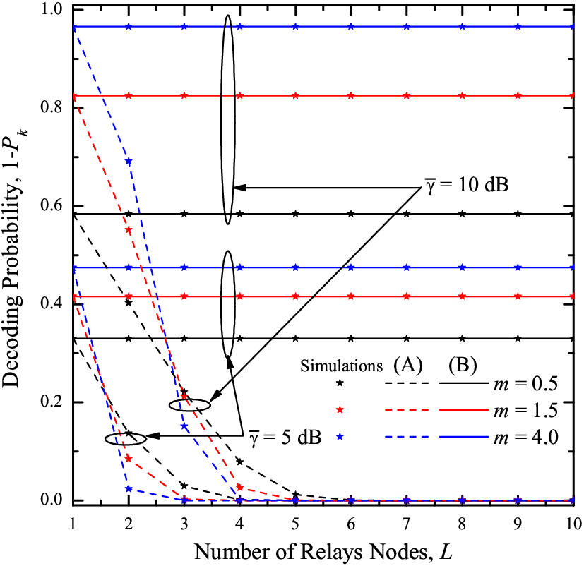
Using (7) in Fig. 4, the decoding probability 1−𝒫k1-\mathcal{P}_{k} is plotted versus LL for both repetitive and RS-based transmission over IID Nakagami-mm fading conditions for the source to relay channels with different values of mm and γ¯L+k=γ¯\overline{\gamma}_{L+k}=\overline{\gamma} ∀k,L\forall\,k,L. As expected, decreasing mm and/or γ¯\overline{\gamma} decreases the decoding probability. Moreover, this probability is severely degraded with increasing LL for repetitive transmission, whereas it remains unchanged with increasing LL for the RS-based one. The PoutP_{\text{out}} performance of pure and rate-selective RS is depicted in Fig. 5 versus γ¯0\overline{\gamma}_{0} for L=2L=2 relays over INID Nakagami-mm fading channels with different values of m0m_{0}, m1m_{1} and m2m_{2}. As expected, for both RS-based schemes, PoutP_{\text{out}} improves with increasing γ¯0\overline{\gamma}_{0} and/or any of the fading parameters. More importantly, it is shown that, as the fading conditions of the relay to destination channels become more favorable than those of the direct source to destination channel, RS-based transmission improves PoutP_{\text{out}}. On the contrary, whenever the fading conditions of the relay to destination channels are similar to the direct one, non-relay assisted transmission results in lower PoutP_{\text{out}} than that of the RS-based one.

In Fig. 6, the P¯b\overline{P}_{\text{b}} performance of square 44-QAM is plotted as a function of LL for average SNR per bit γ¯b=5\overline{\gamma}_{\text{b}}=5 dB for all second hop channels and γ¯0=0\overline{\gamma}_{0}=0 dB over IID Nakagami-mm fading channels with different values of mm. It is clearly shown that the P¯b\overline{P}_{\text{b}} of RS-based transmission improves with increasing LL and/or mm whereas for both repetitive schemes, although P¯b\overline{P}_{\text{b}} improves with increasing mm, it does not benefit from increasing LL. Interestingly, for RS-based transmission, as LL and/or mm increase, the P¯b\overline{P}_{\text{b}} improvement of pure compared with rate-selective RS increases; as shown in (38), rate-selective RS might choose the direct transmission even in cases where the received SNR from the best relay is larger that from the source node. Assuming IID Rayleigh fading conditions, Fig. 7 illustrates P¯b\overline{P}_{\text{b}} of DBPSK versus LL for all considered relaying schemes and for different values of γ¯0\overline{\gamma}_{0}. As shown from this figure and Fig. 6 for both repetitive and RS-based transmission, P¯b\overline{P}_{\text{b}} for both modulations improves with increasing γ¯0\overline{\gamma}_{0} and/or mm. It was shown in Fig. 4 that more favorable fading conditions and larger γ¯0\overline{\gamma}_{0} increase the decoding probability, thus both repetitive transmission schemes become unavailing for larger LL, whereas the gains from RS increase. The P¯b\overline{P}_{\text{b}} performance of DBPSK of pure and rate-selective RS is depicted in Fig. 8 versus γ¯b\overline{\gamma}_{\text{b}} for all second hop channels with L=1L=1, 22 and 33 relays and for γ¯0=0\overline{\gamma}_{0}=0 dB over INID Nakagami-mm fading channels with different values for the fading parameters. Clearly, for both RS-based transmission schemes, P¯b\overline{P}_{\text{b}} improves with increasing γ¯b\overline{\gamma}_{\text{b}} and/or mm and/or LL. It is shown that, as γ¯b\overline{\gamma}_{\text{b}} increases and as the fading conditions of the relay to destination channels become more favorable than those of the direct source to destination channel, RS-based transmission results in larger P¯b\overline{P}_{\text{b}} improvement. More importantly, even for strong source to destination channel conditions, as γ¯b\overline{\gamma}_{\text{b}} increases the improvement on P¯b\overline{P}_{\text{b}} with RS-based transmission becomes larger than that with the non-relay assisted one.

VI Conclusion

Cooperative diversity is a very promising avenue for future wireless communications. However, it is necessary to investigate how relays should be utilized in order to achieve certain objectives. In this paper, we presented a general analytical framework for modelling and evaluating performance of four DF relaying schemes under INID Nakagami-mm fading channels. Moreover, we obtained closed-form expressions for the OP and the ASEP performance of the RS and repetitive schemes when MRD or SD are employed at the destination node. We concluded that RS performs better than repetitive transmission when CSI for RS is perfect. Furthermore, it was shown that relaying should be switched-off when the source to destination direct link is sufficiently strong and the aim is minimizing OP. However, in terms of ASEP, relaying was shown to be always beneficial.

References

  • [1] G. J. Foschini and M. J. Gans, “On limits of wireless communications in a fading environment when using multiple antennas,” IEEE Trans. Veh. Technol., vol. 6, no. 3, pp. 311–335, Mar. 1998.
  • [2] E. Biglieri, R. Calderbank, A. Constantinides, A. Goldsmith, A. Paulraj, and H. V. Poor, MIMO wireless communications, 1st ed. Cambridge: Cambridge University Press, 2007.
  • [3] J. N. Laneman and G. W. Wornell, “Distributed space-time coded protocols for exploiting cooperative diversity in wireless networks,” IEEE Trans. Inf. Theory, vol. 49, no. 10, pp. 2415–2425, Oct. 2003.
  • [4] A. Sendonaris, E. Erkip, and B. Aashang, “User coorperation diversity - part I: System description,” IEEE Trans. Commun., vol. 51, no. 11, pp. 1927–1938, Nov. 2003.
  • [5] A. Papadogiannis, G. C. Alexandropoulos, A. G. Burr, and D. Grace, “Bringing mobile relays for wireless access networks into practice– learning when to relay,” submitted to IET Communications, Feb. 2011.
  • [6] A. Bletsas, A. Khisti, D. P. Reed, and A. Lippman, “A simple cooperative diversity method based on network path selection,” IEEE J. Sel. Areas Commun., vol. 24, no. 8, pp. 659–672, Mar. 2006.
  • [7] A. Papadogiannis, E. Hardouin, A. Saadani, D. Gesbert, and P. Layec, “A novel framework for the utilization of dynamic relays in cellular networks,” in Proc. IEEE ASIMOLAR 2008, Pacific Grove, USA, Oct. 2008.
  • [8] A. Papadogiannis, A. Saadani, and E. Hardouin, “Exploiting dynamic relays with limited overhead in cellular systems,” in Proc. IEEE GLOBECOM Workshops 2009, Hawaii, USA, Nov. 2009, pp. 1–6.
  • [9] K. Yan, J. Jiang, Y. G. Wang, and H. T. Liu, “Outage probability of selection cooperation with MRC in Nakagami-mm fading channels,” IEEE Signal Process. Lett., vol. 16, no. 12, pp. 1031–1034, Dec. 2009.
  • [10] G. C. Alexandropoulos, A. Papadogiannis, and K. Berberidis, “Performance analysis of cooperative networks with relay selection over Nakagami-mm fading channels,” IEEE Signal Process. Lett., vol. 17, no. 5, pp. 1–4, May 2010.
  • [11] N. C. Beaulieu and J. Hu, “A closed-form expression for the outage probability of decode-and-forward relaying in dissimilar Rayleigh fading channels,” IEEE Commun. Lett., vol. 10, no. 12, pp. 813–815, Dec. 2006.
  • [12] J. Hu and N. C. Beaulieu, “Performance analysis of decode-and-forward relaying with selection combining,” IEEE Commun. Lett., vol. 11, no. 6, pp. 489–491, Jun. 2007.
  • [13] E. Beres and R. Adve, “Selection cooperation in multi-source cooperative networks,” IEEE Trans. Wireless Commun., vol. 7, no. 1, pp. 118–127, Jan. 2008.
  • [14] F. Xu, F. C. M. Lau, Q. F. Zhou, and D.-W. Yue, “Outage performance of cooperative communication systems using opportunistic relaying and selection combining receiver,” IEEE Signal Process. Lett., vol. 16, no. 4, pp. 237–240, Apr. 2009.
  • [15] C. K. Datsikas, N. C. Sagias, F. I. Lazarakis, and G. S. Tombras, “Outage analysis of decode-and-forward relaying over Nakagami-mm fading channels,” IEEE Signal Process. Lett., vol. 15, no. 1, pp. 41–44, Jan. 2008.
  • [16] A. Papadogiannis and G. C. Alexandropoulos, “System level performance evaluation of dynamic relays in cellular networks over Nakagami-mm fading channels,” in Proc. IEEE PIMRC 2009, Tokyo, Japan, Sep. 2009.
  • [17] G. C. Alexandropoulos, A. Papadogiannis, and K. Berberidis, “Relay selection vs. repetitive transmission cooperation: Analysis over Nakagami-mm fading channels,” in Proc. IEEE PIMRC 2010, Istanbul, Turkey, Sep. 2010.
  • [18] Q. T. Duong, G. C. Alexandropoulos, H.-J. Zepernick, and T. A. Tsiftsis, “Orthogonal space-time block codes with CSI-assisted amplify-and-forward relaying in correlated Nakagami-mm fading channels,” IEEE Trans. Veh. Technol., vol. 60, no. 3, pp. 882–889, Mar. 2011.
  • [19] I. S. Gradshteyn and I. M. Ryzhik, Table of Integrals, Series, and Products, 6th ed. New York: Academic, 2000.
  • [20] M. Nakagami, “The mm-distribution - A general formula of intensity distribution of rapid fading,” in Statistical Methods in Radio Wave Propagation, W. G. Hoffman, Ed. Oxford, UK: Permagon Press, 1960, pp. 3–36.
  • [21] M. K. Simon and M.-S. Alouini, Digital Communication over Fading Channels, 2nd ed. New York: Wiley, 2005.
  • [22] K. Woradit, T. Q. S. Quek, W. Suwansantisuk, H. Wymeersch, L. Wuttisittikulkij, and M. Z. Win, “Outage behavior of cooperative diversity with relay selection,” in Proc. IEEE GLOBECOM 2008, New Orleans, L.A., USA, Dec. 2008.
  • [23] W. G. Cochran, Sampling Techniques, 3rd ed. New York: Wiley, 1977.

FIGURES’ CAPTIONS

Fig. 1: Illustration of a dual-hop cooperative wireless system with L+2L+2 wireless nodes: a source node SS, LL relay station nodes RkR_{k}, k=1,2,…,Lk=1,2,\ldots,L, and a destination node DD.

Fig. 2: End-to-end OP, PoutP_{\text{out}}, versus the number of relay nodes, LL, for average transmit SNR γ¯0=5\overline{\gamma}_{0}=5 dB over IID Nakagami-mm fading channels with different values of mm: (A) Pure RS, (B) Rate-Selective RS, (C) Repetitive transmission with MRD and (D) Repetitive transmission with SD.

Fig. 3: End-to-end OP, PoutP_{\text{out}}, versus the number of relay nodes, LL, for different average transmit SNRs over IID Rayleigh fading channels: (A) Pure RS, (B) Rate-Selective RS, (C) Repetitive transmission with MRD and (D) Repetitive transmission with SD.

Fig. 4: Decoding probability, 1−𝒫k1-\mathcal{P}_{k}, versus the number of relay nodes, LL, over IID Nakagami-mm fading channels with different values of mm and γ¯L+k=γ¯\overline{\gamma}_{L+k}=\overline{\gamma} ∀k,L\forall\,k,L: (A) Repetitive and (B) RS-based transmission.

Fig. 5: End-to-end OP, PoutP_{\text{out}}, of RS versus the average transmit SNR per bit, γ¯0\overline{\gamma}_{0}, for L=2L=2 relay nodes over INID Nakagami-mm fading channels: (A) m0=m1=m2=1m_{0}=m_{1}=m_{2}=1 and δ=0.3\delta=0.3, (B) m0=1m_{0}=1, m1=m2=6m_{1}=m_{2}=6 and δ=0.3\delta=0.3 and (C) m0=m1=m2=3m_{0}=m_{1}=m_{2}=3 and δ=0\delta=0.

Fig. 6: ABEP, P¯b\overline{P}_{\text{b}}, of square 44-QAM versus the number of relay nodes, LL, for average transmit SNR γ¯b=5\overline{\gamma}_{\text{b}}=5 dB and γ¯0=0\overline{\gamma}_{0}=0 dB over IID Nakagami-mm fading channels with different values of mm: (A) Pure RS, (B) Rate-Selective RS, (C) Repetitive transmission with MRD and (D) Repetitive transmission with SD.

Fig. 7: ABEP, P¯b\overline{P}_{\text{b}}, of DBPSK versus the number of relay nodes, LL, for different average transmit SNRs per bit and γ¯0=0\overline{\gamma}_{0}=0 dB, over IID Rayleigh fading channels: (A) Pure RS, (B) Rate-Selective RS, (C) Repetitive transmission with MRD and (D) Repetitive transmission with SD.

Fig. 8: ABEP, P¯b\overline{P}_{\text{b}}, of DBPSK for RS versus the average relay SNR per bit, γ¯b\overline{\gamma}_{\text{b}}, and for γ¯0=0\overline{\gamma}_{0}=0 dB over INID Nakagami-mm fading channels: (A) L=1L=1, m0=0.5m_{0}=0.5, m1=1m_{1}=1 and δ=0.1\delta=0.1, (B) L=2L=2, m0=1m_{0}=1, m1=m2=2m_{1}=m_{2}=2 and δ=0\delta=0 and (C) L=3L=3, mℓ=3m_{\ell}=3 for ℓ=0,1,2\ell=0,1,2 and 33 and δ=0\delta=0.

Refer to caption
Fig. 1: Illustration of a dual-hop cooperative wireless system with L+2L+2 wireless nodes: a source node SS, LL relay station nodes RkR_{k}, k=1,2,…,Lk=1,2,\ldots,L, and a destination node DD.
Refer to caption
Fig. 2: End-to-end OP, PoutP_{\text{out}}, versus the number of relay nodes, LL, for average transmit SNR γ¯0=5\overline{\gamma}_{0}=5 dB over IID Nakagami-mm fading channels with different values of mm: (A) Pure RS, (B) Rate-Selective RS, (C) Repetitive transmission with MRD and (D) Repetitive transmission with SD.
Refer to caption
Fig. 3: End-to-end OP, PoutP_{\text{out}}, versus the number of relay nodes, LL, for different average transmit SNRs over IID Rayleigh fading channels: (A) Pure RS, (B) Rate-Selective RS, (C) Repetitive transmission with MRD and (D) Repetitive transmission with SD.
Refer to caption
Fig. 4: Decoding probability, 1−𝒫k1-\mathcal{P}_{k}, versus the number of relay nodes, LL, over IID Nakagami-mm fading channels with different values of mm and γ¯L+k=γ¯\overline{\gamma}_{L+k}=\overline{\gamma} ∀k,L\forall\,k,L: (A) Repetitive and (B) RS-based transmission.
Refer to caption
Fig. 5: End-to-end OP, PoutP_{\text{out}}, of RS versus the average transmit SNR per bit, γ¯0\overline{\gamma}_{0}, for L=2L=2 relay nodes over INID Nakagami-mm fading channels: (A) m0=m1=m2=1m_{0}=m_{1}=m_{2}=1 and δ=0.3\delta=0.3, (B) m0=1m_{0}=1, m1=m2=6m_{1}=m_{2}=6 and δ=0.3\delta=0.3 and (C) m0=m1=m2=3m_{0}=m_{1}=m_{2}=3 and δ=0\delta=0.
Refer to caption
Fig. 6: ABEP, P¯b\overline{P}_{\text{b}}, of square 44-QAM versus the number of relay nodes, LL, for average transmit SNR γ¯b=5\overline{\gamma}_{\text{b}}=5 dB and γ¯0=0\overline{\gamma}_{0}=0 dB over IID Nakagami-mm fading channels with different values of mm: (A) Pure RS, (B) Rate-Selective RS, (C) Repetitive transmission with MRD and (D) Repetitive transmission with SD.
Refer to caption
Fig. 7: ABEP, P¯b\overline{P}_{\text{b}}, of DBPSK versus the number of relay nodes, LL, for different average transmit SNRs per bit and γ¯0=0\overline{\gamma}_{0}=0 dB, over IID Rayleigh fading channels: (A) Pure RS, (B) Rate-Selective RS, (C) Repetitive transmission with MRD and (D) Repetitive transmission with SD.
Refer to caption
Fig. 8: ABEP, P¯b\overline{P}_{\text{b}}, of DBPSK for RS versus the average relay SNR per bit, γ¯b\overline{\gamma}_{\text{b}}, and for γ¯0=0\overline{\gamma}_{0}=0 dB over INID Nakagami-mm fading channels: (A) L=1L=1, m0=0.5m_{0}=0.5, m1=1m_{1}=1 and δ=0.1\delta=0.1, (B) L=2L=2, m0=1m_{0}=1, m1=m2=2m_{1}=m_{2}=2 and δ=0\delta=0 and (C) L=3L=3, mℓ=3m_{\ell}=3 for ℓ=0,1,2\ell=0,1,2 and 33 and δ=0\delta=0.