Ergodic Transmission Capacity of Wireless Ad Hoc Networks with Interference Management

In the literature on wireless network throughput (see [1, 3, 4, 5, 2, 6, 7] and the references therein), a unified and time-invariant channel model is typically adopted over the entire network, but channels in a large-scale wireless network usually are diverse across time and/or space. Using a channel model without temporal correlation does not capture how channel states evolve over time and thus the impact on network throughput from the temporal (and spatial) variations of channels is ignored, and techniques which exploit the variations and correlations cannot be properly quantified. For example, we observe that transmission techniques that increase the snapshot network throughput may not increase ETC or may even degrade it. In particular, we will show that channel-aware opportunistic transmission (CAOT), i.e. transmitting when channels are in good states, does not always improve ETC, which is perhaps surprising.

ETC requires the use of different channel models that include temporal discrepancies. We propose a finite-state Markov chain (FSMC) to model the fading channels, in particular a $m$-state Markov chain that is irreducible and positive recurrent. Each channel undergoes path loss and fading and has an ergodic property in that its fading state has an invariant (steady-state) probability [8]. This idea can be traced back to the early work of Gilbert and Elliott [9][10] that used a two-state Markov chain to represent good and bad channel conditions which was extended to a finite state case in [11].

The first contribution in this paper is the model for ETC itself. We then calculate the ETC, which requires the outage probability for each fading channel state to be found, for which we find tight closed-form bounds based on a proposed $\delta$-level interfering coverage area around a receiver. Any single transmitter in the $\delta$-level region of its unintended receiver will cause an outage if its interference power is enlarged by a factor $\delta$. We show that appropriately choosing $\delta$ admits bounds on outage probability that are much tighter than those found in previous work.

Bounds on ETC and their corresponding scaling laws for some special cases are then found. They reveal several interesting implications, e.g. the scaling of ETC for a sparse or dense network is

where $C_{\texttt{E}}$ denotes ETC, $\mathbf{s}_{\epsilon}=\left[\tilde{s}^{\frac{2}{\alpha}}_{1},\tilde{s}^{\frac{2}{\alpha}}_{2},\cdots,\tilde{s}^{\frac{2}{\alpha}}_{m}\right]^{\textsf{T}}$ in which $\tilde{s}_{k}$ is the function of the $k$th state $s_{k}$ of a Markov fading channel with $m$ states, $\Phi=[\phi_{1}\,\,\phi_{2}\,\cdots\,\,\phi_{m}]^{\textsf{T}}\in[0,1]^{m}$ is the invariant probability vector¹¹ 1 The physical meaning of $\phi_{k}$ is the fraction of time that channel state $s_{k}$ sojourns as time goes to infinity. of the Markov fading channel model and $\alpha>2$ is the path loss exponent. From (1), we notice that a single deep fading state is not necessary to have a significant negative effect on ETC if its invariant probability is very small. This point is not revealed in prior work that neglects temporal variations. Also, we observe that ETC has a geometric interpretation because it can be viewed as an inner product of two vectors. Thus, ETC is maximized when the directions of $\Phi_{k}$ and $\mathbf{s}_{\epsilon}$ coincide. In addition, we show that channel-aware opportunisitc transmission (CAOT), which is a scheme to allow transmitters to transmit only when their channels are in good states, does not necessarily provide an ETC gain. Although CAOT is able to increase the transmission capacity contributed by good channel states, it loses the transmission capacity contributed by bad channel states. So CAOT cannot benefit ETC if the improvement is no larger than the loss from bad channel states.

Three interference management methods – avoidance, suppression and cancellation – are applied to the network to reduce outage probability. Bounds on the outage probability and ETC with interference management are found which provide geometric insight into the efficiency of each technique in different scenarios. For example, we show that interference cancellation is not effective for significantly increasing ETC in a spare or dense network. Also, we show interference management can control the direction and magnitude of vector $\mathbf{s}_{\epsilon}$. Finally, we show that CAOT should not be used if interference management can significantly lower interference.

The wireless network considered in this paper is of infinite size and all nodes in the network are independently and randomly scattered. Thus, we employ a marked homogeneous Poisson point process (PPP) $\Pi$ on the plane $\mathbb{R}^{2}$ to represent the locations of all transmitting nodes in the network, which can be written at time $\tau$ as²² 2 Here it is better to use $\Pi(\tau)$ instead of $\Pi$. However, to simplify notation, we will use $\Pi$ to stand for $\Pi(\tau)$ throughout this paper if ignoring time indices does not induce any ambiguity. This custom is applied to other set and variable notations.

where $X_{i}$ denotes node $X_{i}$ as well as its location, $H_{i}(\tau)$ is the fading channel gain between node $X_{i}$ and its receiver $Y_{i}$, and $e_{i}(\tau)\in\{0,1\}$ represents the transmitting index of node $X_{i}$: $e_{i}(\tau)=1$ means node $X_{i}$ is transmitting; otherwise, it is idle. The intensity (density) of $\Pi$ is $\lambda$ for all $\tau\in\mathbb{N}$.

Each transmitter has a unique receiver and the distance between a TX-RX pair is a constant $d>1$. All of the transmitters use the same transmit power and the channel model between each TX-RX pair is subject to path loss and fading. So the channel gain for TX-RX pair $i$ can be written as

where $H_{i}(\tau)$ is the fading channel gain, $|X_{i}-Y_{i}|$ denotes the Euclidean distance between nodes $X_{i}$ and $Y_{i}$ and $\ell(|\cdot|)$ is the path loss function. In order to avoid the singularity where $|X\rightarrow 0$, we will use

where $\alpha>2$ is the path loss exponent³³ 3 In a planar network, we require $\alpha>2$ to have bounded interference, i.e. $I_{t}<\infty$ almost surely if $\alpha>2$ [12, 13]. and $\mathds{1}(x\in\mathcal{X})$ denotes the indicator function: $\mathds{1}(x\in\mathcal{X})=1$ if $x\in\mathcal{X}$ and 0, otherwise.

Specifically, we use an $m$-state FSMC model to characterize the fading effect of all channels in the network. The FSMC is irreducible and positive recurrent, and its $m$ states are ordered. The FSMC model with transition matrix $\mathbf{P}$ is denoted by $\mathcal{S}(\mathbf{P})\in\mathbb{R}_{+}^{m}$ and $\mathcal{S}$ is an order set of the $m$ states, i.e. for any two states $s_{i},s_{j}\in\mathcal{S}$ we have $s_{i}<s_{j}$ where $i<j$ and $i,j\in\mathcal{M}\triangleq\{1,2,\cdots,m\}$. Since $\mathcal{S}$ is irreducible and positive recurrent, the fading channel gain $H(\tau)$ for all TX-RX pairs must satisfy the following conditions[8]:

where $\Phi\triangleq[\phi_{1},\phi_{2},\cdots,\phi_{m}]^{\textsf{T}}$ is the invariant probability vector of $\mathbf{P}$ and $\mathbf{u}\triangleq[1\,\,1\,\cdots\,1]^{\textsf{T}}$ is an $m$-tuple vector. Namely, at any time $\tau$, $H(\tau)$ must belong to one of the states in $\mathcal{S}$ and $\phi_{k}$ represents the probability that $H(\tau)$ visits state $s_{k}$ in a long-term sense. We can show this $m$-state Markov channel model has a temporal ergodic property as stated in the following lemma.

Consider the typical TX-RX pair and its steady state outage probability is

where $q_{k}(\lambda)\triangleq\lim_{\tau\rightarrow\infty}\mathbb{P}[\mathrm{SIR}(\tau,\lambda)<\beta|H(\tau)=s_{k}]$ is the outage probability for channel state $s_{k}$ as time $\tau$ goes to infinity. Now we are ready to use (9) to define ergodic transmission capacity in this paper.

The definition of $C_{\texttt{E}}$ in (10) originates from the following definition:

Since all channels are an irreducible and positive current Markov chain, according to Lemma 1 they all have temporal ergodicity. Thus, the definition in (11) is equivalent to $C_{\texttt{E}}=b\,\bar{\lambda}_{\texttt{E}}\sum_{k=1}^{m}\phi_{k}[1-q_{k}(\bar{\lambda}_{\texttt{E}})]$. This is the reason why we directly use the invariant probability of a Markov chain to define ETC instead of using (11). For ease of analysis, we need to quantitatively define the sparseness and denseness of a network with Poisson-distributed nodes.

Since a closed-form expression of the outage probability defined in (9) is difficult to find⁴⁴ 4 If all channels are instead Rayleigh fading, the closed-form of the outage probability can be found by the Laplace transform of the aggregate interference contributed by Poisson-distributed transmitters[12][18]. However, such closed-form outage probability cannot be obtained for the case of channels without fading [2][19] or with a single state at any time., we resort to bounds. The idea of approaching the lower bound for a receiver with channel state $s_{k}$ is to use a $\delta$-level interfering coverage $\mathcal{I}^{\delta}_{k}$ for the typical receiver $Y_{0}$ with fading state $s_{k}$, and it is defined as follows⁵⁵ 5 If $\delta=1$, then $\mathcal{I}^{\delta}_{k}$ is called the dominant interferer coverage in which a single interferer causes outage at receiver $Y_{0}$.:

which means any single interferer within it can cause outage at receiver $Y_{0}$ with a SIR threshold $\delta\beta$. If $\mathcal{I}^{\delta}_{k}$ is not empty, it could contain dominant interferers and non-dominant interferers. In addition, $\Pi_{k}^{\delta}\triangleq(\Pi\cap\mathcal{I}^{\delta}_{k})\setminus X_{0}$ is called $\delta$-level interfering point process.

The lower bound on the outage probability $q_{k}(\lambda)$ can be acquired by considering the outage events caused by $\Pi^{\delta}_{k}$. The upper bound can be approached by finding the probability of the union outage events separately caused by the interferers in $\Pi^{\delta}_{k}$ and $\Pi\setminus\Pi^{\delta}_{k}$. These two bounds found are tighter than those in the previous works[2][19], as the following theorem shows.

By using the bounds on the outage probability of each channel state in Theorem 1, the ETC in (10) has bounds as shown in the following theorem.

In the previous subsection, we have obtained bounds on ETC and discussed the scaling laws of ETC for a sparse and dense network. From the bounds and scaling laws, we have made three interesting observations.

ETC implicitly possesses a geometric interpretation. The scaling law of ETC in (19) can be expressed in a general form by vectors $\Phi$ and $\mathbf{s}_{\epsilon}$ as

where $\Phi=[\phi_{1},\phi_{2},\cdots,\phi_{m}]^{\textsf{T}}$ and $\mathbf{s}$ is defined as

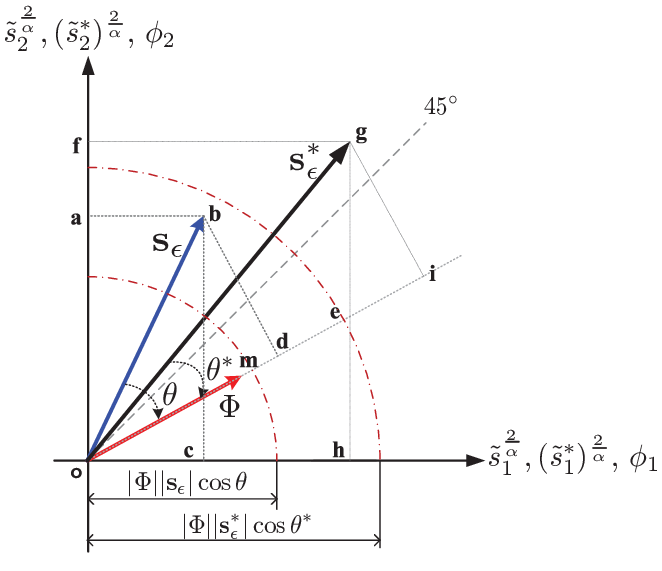
In other words, $C_{\texttt{E}}$ is scaled by the inner product of vectors $\Phi$ and $\mathbf{s}_{\epsilon}$. So the result in (22) can be interpreted from a geometric point of view. Suppose the Markov channel model has two fading states (i.e. $m=2$, this is so called Gilbert-Elliott channel model[9][10]). Then $C_{\texttt{E}}$ in (22) can be schematically presented in Fig. 2. Note that $\mathbf{s}_{\epsilon}$ must be above on the $45^{\circ}$ line because $s_{2}$ is larger than $s_{1}$. The inner product of $\mathbf{s}_{\epsilon}$ and $\Phi$ can be written as $\Phi^{\textsf{T}}\mathbf{s}_{\epsilon}=|\Phi||\mathbf{s}_{\epsilon}|\cos\theta$ and $\theta$ is the angle between vectors $\mathbf{s}_{\epsilon}$ and $\Phi$. So we will have a larger ETC if $\Phi$ has the same direction as $\mathbf{s}_{\epsilon}$. The optimal $\Phi_{*}$ that maximizes ETC can be given by $\Phi_{*}=\frac{\mathbf{s}_{\epsilon}}{\mathbf{u}^{\textsf{T}}\mathbf{s}_{\epsilon}}$. Therefore, if all Markov fading channels have the optimal distribution $\Phi_{*}$, then $C_{\texttt{E}}$ in (22) becomes

and thus it is completely characterized by all channel fading states.

Dominant channel states may not dominate ETC. Dominant states in a Markov chain means that their invariant probabilities are much larger than other states’ invariant probabilities. In other words, if a channel has dominant states then it is in these states most of the time. Dominant channel states may not contribute too much ETC since their state magnitudes could be very small (very bad states). Thus, dominant channel states which really dominates ETC only when they have a large magnitude. This point can also be visually explained by Fig. 2. Suppose $s_{2}$ dominates and it is much larger than $s_{1}$. In this case, $\Phi$ and $\mathbf{s}_{\epsilon}$ will move up and be close to the vertical axis. The projection of $\Phi$ on $\mathbf{s}_{\epsilon}$ will largely increase and it is mostly contributed by the vertical component. Thus, whether a channel state dominates ETC or not depends on the product of its magnitude and invariant probability.

CAOT may not benefit ETC. If we compare the results in Theorem 2 and Corollary 1, we can find CAOT indeed increases the bounds with good channel states. Nevertheless, it may not always improve ETC since it loses the throughput contributed by bad channel states. To show this, let the upper bound in (17) be greater than the upper bound in (21). This leads to the following inequality:

The LHS in the above expression is the ETC improved by CAOT and the RHS is the ETC loss because of bad channel states. If this inequality is valid, apparently CAOT may not improve ETC because the ETC increase in the good states could not compensate the ETC loss in the bad states. Hence, following from (25), the better policy of using CAOT for a transmitter is when the following condition holds

However, the above condition is not implementable by transmitters in a wireless ad hoc network without knowing $\Phi$ in advance. So CAOT is not always an effective means to enhance ETC in a real-time situation. A simulation example for ETC with and without CAOT is shown in Fig. 3. Channel fading is modeled by a 2-state Markov chain and the simulation condition is set to let the bad channel state be dominant. Obviously, we can see that ETC with CAOT is worse than ETC without CAOT.

Interference management can be classified into three categories: interference avoidance, suppression and cancellation. Avoiding interference in a wireless ad hoc network is typically accomplished by using space, time or frequency orthogonality to eliminate the co-reception of strong interferers. Frequency-hopping and CSMA are prominent examples of avoiding interference in an ad hoc network. Interference suppression deploys signal processing at the transmitter and/or receiver to (linearly) suppress interference without actually cancelling it. Direct-Sequence CDMA (DS-CDMA) is a typical example of this category. In addition, receivers can try to cancel strong interference from their nearby unintended transmitters (e.g. successive interference cancellation (SIC)[21, 22, 23]). Although avoiding interference and suppressing interference are two different methods of reducing interference, we know there exists a duality property between them in a wireless network with Poisson-distributed nodes. According to the conservation property of a homogeneous PPP[17]⁶⁶ 6 The conservation property of a homogeneous PPP with intensity $\lambda$ is that the intensity will change to $\lambda/a$ if all locations of the nodes in the PPP are scaled by a constant $\sqrt{a}$., these two methods both reduce the original intensity of transmitters so that their effect can be demonstrated via another homogeneous PPP with a new intensity. However, interference avoidance has a better efficiency in reducing the intensity of interferers than interference suppression[2][20].

The effect of interference cancellation can also be grasped from a geometric perspective. To explain this, suppose now any receiver $Y_{i}$ in the network is able to cancel some interference from its nearby interferers after the interference is avoided and/or suppressed. As time goes to infinity, the interference cancellation coverage of receiver $Y_{0}$ with channel state $s_{k}$ is defined in the following.

where $I_{0}$ is the interference of receiver $Y_{0}$ and $\gamma_{k}\in(0,1)$ is called interference reduction factor for channel state $s_{k}$⁷⁷ 7 Reduction factor $\gamma_{k}$ can account for the joint effect of interference avoidance and suppression. For example, if there are $M>1$ available channels for DS-CDMA with spreading gain $G>1$, then $\gamma_{k}=1/GM^{\frac{\alpha}{2}}$.. Coverage $\mathcal{C}^{\texttt{c}}_{k}$ means that any received interference within this region can be decoded by receiver $Y_{0}$ with channel state $s_{k}$, and all transmitters in $\mathcal{C}^{\texttt{c}}_{k}$ have a larger received power than transmitter $X_{0}$ if $\mathcal{C}^{\texttt{c}}_{k}\cap(\Pi\setminus X_{0})$ is not empty and $\beta>1$. Also, $\mathcal{C}^{\texttt{c}}_{k}$ is a random compact set so that its mean Lebesgue measure $\mu(\mathcal{C}^{\texttt{c}}_{k})$ is finite. If each receiver can perfectly cancel all interferers in its cancellation coverage after suppressing and/or avoiding some interference, then its SIR for channel state $s_{k}$ is

where $\Pi_{k}^{\texttt{nc}}\triangleq\Pi\setminus(\mathcal{C}^{\texttt{c}}_{k}\cap\Pi\cup X_{0})$ is the noncancelable part of $\Pi$ with intensity $\lambda\gamma^{\frac{2}{\alpha}}_{k}$. So equation (28) essentially suggests that interference management can be equivalently reflected by constructing a new PPP with a reduced intensity. The above $\mathrm{SIR}_{k}$ expression will be used in the following subsection to find the bounds on the outage probability. Those bounds are used to characterize the bounds on ETC with interference management.

Bounds on the outage probability with interference management are shown in the following theorem.

According to the bounds on the outage probability in Theorem 3, ETC with interference management is bounded as shown in the following theorem.

References

- [1] P. Gupta and P. R. Kumar, “The capacity of wireless networks,” IEEE Trans. Inf. Theory, vol. 46, no. 2, pp. 388–404, Mar. 2000.
- [2] S. Weber, X. Yang, J. G. Andrews, and G. de Veciana, “Transmission capacity of wireless ad hoc networks with outage constraints,” IEEE Trans. Inf. Theory, vol. 51, no. 12, pp. 4091–4102, Dec. 2005.
- [3] J. Li, C. Blake, D. S. J. D. Couto, H. I. Lee, and R. Morris, “Capacity of ad hoc wireless networks,” in Proc. IEEE International Conf. on Mobile Computing and Networking (MobiCom’01), Jul. 2001.
- [4] S. R. Kulkarni and P. Viswanath, “A deterministic approach to throughput scaling in wireless networks,” IEEE Trans. Inf. Theory, vol. 50, no. 6, pp. 1041–1049, Jun. 2004.
- [5] R. Negi and A. Rajeswran, “Capacity of power constrained ad-hoc networks,” in Proc. IEEE INFOCOM, Apr. 2004.
- [6] F. Xue and P. R. Kumar, Scaling Laws for Ad Hoc Wireless Networks: An Information Theoretic Approach. Now Publishers: Foundations and Trends in Networking, 2006.
- [7] S. Weber, J. G. Andrews, and N. Jindal, “The effect of fading, channel inversion, and threshold scheduling on ad hoc networks,” IEEE Trans. Inf. Theory, vol. 53, no. 11, pp. 4127–4149, Nov. 2007.
- [8] S. Meyn and R. L. Tweedie, Markov Chains and Stochastic Stability, 2nd ed. Cambridge University Press, 2009.
- [9] E. N. Gilbert, “Capacity of a burst-noise channel,” Bell Syst. Tech. J., vol. 39, no. 9, pp. 1253–1265, Sep. 1960.
- [10] E. O. Elliott, “Estimates of error rates for codes on burst-noise channels,” Bell Syst. Tech. J., vol. 42, no. 9, pp. 1977–1997, Sep. 1963.
- [11] H. S. Wang and N. Moayeri, “Finite-state markov channel - a useful model for radio communication channels,” IEEE Trans. Veh. Technol., vol. 44, no. 1, pp. 163–171, Feb. 1995.
- [12] F. Baccelli, B. Blaszczyszyn, and P. Mühlethaler, “An Aloha protocol for multihop mobile wireless networks,” IEEE Trans. Inf. Theory, vol. 52, no. 2, pp. 421–436, Feb. 2006.
- [13] M. Haenggi, J. G. Andrews, F. Baccelli, O. Dousse, and M. Franceschetti, “Stochastic geometry and random graphs for the analysis and design of wireless networks,” IEEE J. Sel. Areas Commun., vol. 27, pp. 1029–1046, Sep. 2009.
- [14] S. B. Lowen and M. C. Teich, “Power-law shot noise,” IEEE Trans. Inf. Theory, vol. 36, no. 6, pp. 1302–1318, Sep. 1990.
- [15] J. Ilow and D. Hatzinakos, “Optimum transmission ranges in a direct-sequence spread-spectrum multihop packet radio network,” IEEE Trans. Signal Process., vol. 46, no. 6, pp. 1601–1611, Jun. 1998.
- [16] E. S. Sousa and J. A. Silvester, “Optimum transmission ranges in a direct-sequence spread-spectrum multihop packet radio network,” IEEE J. Sel. Areas Commun., vol. 8, no. 5, pp. 762–771, Jun. 1990.
- [17] D. Stoyan, W. Kendall, and J. Mecke, Stochastic Geometry and Its Applications, 2nd ed. John Wiley and Sons, Inc., 1996.
- [18] J. F. C. Kingman, Poisson Processes. Oxford University Press, 1993.
- [19] S. Weber, J. G. Andrews, X. Yang, and G. de Veciana, “Transmission capacity of wireless ad hoc networks with successive interference cancellation,” IEEE Trans. Inf. Theory, vol. 53, no. 8, pp. 2799–2814, Aug. 2007.
- [20] J. G. Andrews, S. Weber, and M. Haenggi, “Ad hoc networks: To spread or not to spread?” IEEE Commun. Mag., vol. 45, pp. 84–91, Dec. 2007.
- [21] T. Cover, “Broadcast channels,” IEEE Trans. Inf. Theory, vol. IT-18, no. 1, pp. 2–14, Jan. 1972.
- [22] J. G. Andrews, “Interference cancellation for cellular systems: a contemporary overview,” IEEE Wireless Commun. Mag., vol. 12, no. 2, pp. 19–29, Apr. 2005.
- [23] D. N. C. Tse and P. Viswanath, Fundamentals of Wireless Communication. Cambridge University Press, 2005.
- [24] F. Baccelli and B. Błaszczyszyn, Stochastic Geometry and Wireless Networks, Volume I : Theory. Now Publishers: Foundations and Trends in Networking, 2010.