Let $X_{1},...,X_{n}$ be a sequence of independent and identically distributed random variables with distribution function $F$, and let $X_{1,n}\leq...\leq X_{n,n}$ denote the order statistics associated to this sample.

In the present paper, we address the problem of estimating the Weibull tail-coefficient $\theta>0$ defined as

where $\ell$ is a slowly varying function at infinity satisfying

[2] investigated this estimation problem and proposed the following estimator of $\theta$:

where $k_{n}$ is an intermediate sequence, i.e. a sequence such that $k_{n}\to\infty$ and ${k_{n}/n}\to 0$ as $n\to\infty$.

We refer to [15, 13, 4] and [7] for other propositions and to [3] for Local Asymptotic Normality (LAN) results. Estimator (3) is closed in spirit to the Hill estimator [17] in the case of Pareto-type distributions. In [15] , the asymptotic normality of $\widetilde{\theta}_{n}(k_{n})$ is established under suitable assumptions. To prove such a result, a second-order condition is required in order to specify the bias-term. This assumption can be expressed in terms of the slowly varying function $\ell$ as follows:

Assumption $(R_{\ell}(b,\rho))$ There exists a constant $\rho<0$ and a rate function $b$ satisfying $b(x)\to 0$ as $x\to\infty$, such that for all $\varepsilon>0$ and $1<A<\infty$, we have

with $\displaystyle{K_{\rho}(\lambda)=\int_{1}^{\lambda}t^{\rho-1}dt.}$

It can be shown that necessarily $|b|$ is regularly varying with index $\rho$ [14]. Moreover, we focus on the case where the convergence (2) is slow, and thus when the bias term in $\widetilde{\theta}_{n}(k_{n})$ is large. This situation is described by the following assumption:

Let us note that this condition implies $\rho\geq-1$. Gamma and Gaussian distributions fulfill (4), whereas Weibull distributions do not (see Table 1) since, in this case, the bias term vanishes.

Using this framework, we will establish rigorously in Section 2 the following approximation for the log-spacings of upper order statistics:

for $1\leq j\leq k_{n}$, where $(f_{1},...,f_{k_{n}})$ is a vector of independent and standard exponentially distributed random variables. This exponential regression model is similar to the ones proposed by [5, 6] and [11] in the case of Pareto-type distributions. Ignoring $b(\log(n/k_{n}))\Bigr(\frac{\log(n/j)}{\log(n/k_{n})}\Bigr)^{\rho}$ in (5) leads to the maximum likelihood estimator

which turns out to be an alternative estimator of $\widetilde{\theta}_{n}(k_{n})$. The full model (5) allows us to generate bias-corrected estimates $\widehat{\theta}_{n}(k_{n})$ for $\theta$ through maximum likelihood estimation of $\theta$, $b(\log{n/k_{n}})$ and $\rho$ for each $1\leq k_{n}\leq n-1.$ An alternative to this approach consists in using a canonical choice for $\rho$ and to estimate the two other parameters by a least-squares method (LS). For the canonical choice of $\rho$, we can use for instance the value -1, which is the same as the one proposed by [11] for the regression model in the case of Pareto-type distributions. The asymptotic normality of the resulting LS-estimator is established in Section 3. An adaptive selection method for $k_{n}$ in $\check{\theta}_{n}(k_{n})$ is also derived. In order to illustrate the usefulness of these results, we provide a simulation study in Section 4 as well as an application to a real data set in Section 5. The proofs of our results are postponed to Section 7.

In this section, we formalize (5). First, remark that

Since $X_{n-j+1,n}\stackrel{{\scriptstyle d}}{{=}}F^{-1}(U_{n-j+1,n}),1\leq j\leq k_{n},$ where $U_{j,n}$ denotes the $j$-th order statistic of a uniform sample of size $n$, we have

which implies that

Moreover, considering the order statistics from an independent standard exponential sample, $E_{n-j+1,n}\stackrel{{\scriptstyle d}}{{=}}-\log(1-U_{n-j+1,n})$. Therefore

Recall that $Z_{j}=j\log(n/j)\left(\log X_{n-j+1,n}-\log X_{n-j,n}\right)$, $1\leq j\leq k_{n}$. Then, our basic result now reads as follows.

In order to reduce the bias of the estimator $\check{\theta}_{n}(k_{n})$, we can either estimate simultaneously $\theta,b(\log{n/k_{n}})$ and $\rho$ by a maximum likelihood method or estimate $\theta$ and $b$ by a least-squares approach after substituting a canonical choice for $\rho$. In fact, this second-order parameter is difficult to estimate in practice and we can easily check by simulations that fixing its value does not much influence the result. This problem has already been discussed in [5, 6] and [11] where similar observations have been made in the case of Pareto-type distributions. The canonical choice $\rho=-1$ is often used although other choices could be motivated performing a model selection.

We can also take benefit of the estimation of $b(\log n/k_{n})$ by estimating the AMSE given in (7) by:

Then, the intermediate sequence $k_{n}$ can be selected by minimizing the previous quantity:

This adaptive procedure for selecting the number of upper order statistics is in the same spirit as the one used by [19] in the context of the extreme value index estimation.

In order to illustrate the usefulness of the bias reduction and of the selection procedure, we provide a simulation study in the next section.

First, the finite sample performances of the estimators ${\widehat{\theta}}_{n}(k_{n})$, ${\widetilde{\theta}}_{n}(k_{n})$ and ${\check{\theta}}_{n}(k_{n})$ are investigated on 6 different distributions: $\Gamma(0.25,1)$, $\Gamma(4,1)$, $|{\mathcal{N}}|(0,1)$, ${\mathcal{W}}(0.25,0.25)$, ${\mathcal{W}}(4,4)$ and ${\mathcal{D}}(1,0.5)$, see the appendix for the definition of the latter distribution. We limit ourselves to these three estimators, since it is shown in [15] that ${\widetilde{\theta}}_{n}(k_{n})$ gives better results than the other approaches [4, 7]. In each case, $N=100$ samples $({\mathcal{X}}_{n,i})_{i=1,\dots,N}$ of size $n=500$ were simulated. On each sample $({\mathcal{X}}_{n,i})$, the estimates $\widehat{\theta}_{n,i}(k_{n})$, $\widetilde{\theta}_{n,i}(k_{n})$ and $\check{\theta}_{n,i}(k_{n})$ were computed for $k_{n}=2,\dots,360$. Finally, the Hill-type plots were built by drawing the points

We also present the associated MSE plots obtained by plotting the points

Here, the good performance of the adaptive selection procedure is illustrated through the analysis of extreme events on a benchmark real data set. Nidd river data are widely used in extreme value studies [18, 8]. The raw data consist in $154$ exceedances of the level $65$ m³s^-1 by the river Nidd (Yorkshire, England) during the period 1934-1969 (35 years). The $N$-year return level is the water level which is exceeded on average once in $N$ years. Hydrologists need to estimate extreme quantiles in order to predict return levels over long periods. According to [18], the Nidd data may reasonably be assumed to come from a distribution in the Gumbel maximum domain of attraction. This suggests to consider Weibull tail-distributions as a possible model for such data. 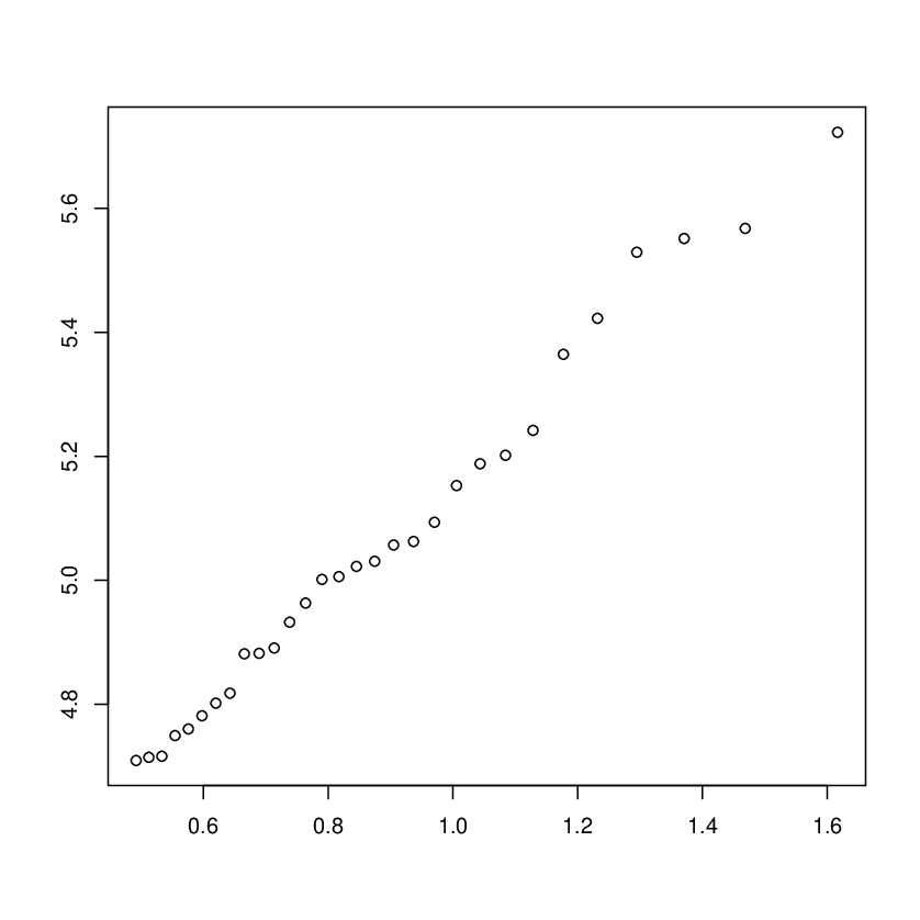The adaptive selection procedure yields $\widehat{k}_{n}=29$. The resulting quantile-quantile plot (obtained by plotting the points $(\log\log(n/i),\log{(X_{n-i+1,n})})$ for $i=1,\dots,\widehat{k}_{n}-1$) is approximatively linear (see Figure 7), indicating a good fit of the Weibull tail-distribution for $x\geq X_{n-\hat{k}_{n}+1,n}$. We obtained $\check{\theta}_{n}(\hat{k}_{n})\simeq\widetilde{\theta}_{n}(\hat{k}_{n})\simeq 0.89$. One can plug this result in the Weissman-type extreme quantile estimator proposed in [12] to obtain $366m^{3}s^{-1}$ as an estimation of the 100-year return level. Note that this result is in accordance with the results obtained by profile-likelihood or Bayesian methods, see [9] or [8].

In this paper, we introduce a regression model, from which we derive a bias-reduced estimator for the Weibull tail-coefficient $\theta$. Its asymptotic normality is established and an adaptive selection procedure for $k_{n}$ is proposed. The efficiency of our approach is illustrated in a simulation study and on a real data set. However, in many cases of practical interest, the problem of estimating a quantile $x_{p_{n}}=F^{-1}(1-p_{n})$, with $p_{n}<1/n$, is much more important. Such a problem has already been studied in [12] where the following Weissman-type estimator has been introduced

It is, however, desirable to refine $\widetilde{x}_{p_{n}}(k_{n})$ with the additional information about the slowly varying function $\ell$ that is provided by the LS-estimates for $\theta$ and $b$. To this aim, condition $(R_{\ell}(b,\rho))$ is used to approximate the ratio $F^{-1}(1-p_{n})/X_{n-k_{n}+1,n}$, noting that

with $U_{1,n}\leq...\leq U_{n,n}$ the order statistics of a uniform $(0,1)$ sample of size $n$,

The last step follows from replacing $U_{k_{n}+1,n}$ (resp. $E_{n-k_{n}+1,n}$) by $k_{n}/n$ (resp. $\log(n/k_{n})$). Hence, we arrive at the following estimator for extreme quantiles

which is similar to the estimator proposed by [20] in the case of Pareto-type distributions. Here, the LS-estimators of $\theta$ and $b$ can be used after substituting $\rho$ by the canonical choice $-1$. The study of the asymptotic properties of such an estimator is the aim of [10].

References

[1] Abramowitz, M., Stegun, I., (1972),
Handbook of Mathematical Functions, Dover.
[2]
Beirlant, J., Teugels, J. and Vynckier, P., (1996)
Practical analysis of extreme values,
Leuven university press.
[3]
Beirlant, J., Bouquiaux, C., Werker, B., (2005),
Semiparametric lower bounds for tail index estimation,
Journal of Statistical Planning and Inference, to appear.
[4] Beirlant, J., Broniatowski, M., Teugels, J.L., Vynckier, P., (1995),
The mean residual life function at great age: Applications to tail estimation,
Journal of Statistical Planning and Inference, 45, 21–48.
[5] Beirlant, J., Dierckx, G., Goegebeur, Y., Matthys, G., (1999),
Tail index estimation and an exponential regression model,
Extremes, 2, 177–200.
[6] Beirlant, J., Dierckx, G., Guillou, A., Starica, C., (2002),
On exponential representations of log-spacings of extreme order statistics,
Extremes, 5 (2), 157–180.
[7] Broniatowski, M., (1993),
On the estimation of the Weibull tail coefficient,
Journal of Statistical Planning and Inference, 35, 349–366.
[8]
Davison, A.C. and Smith, R.L., (1990)
Models for exceedances over high thresholds,
Journal of the Royal Statistical Society B,
52(3), 393–442.
[9]
Diebolt, J., El-Aroui, M., Garrido, M. and Girard, S. (2005)
Quasi-conjugate Bayes estimates for GPD parameters and application to heavy tails modelling,
Extremes,
8, 57–78.
[10]
Diebolt, J., Gardes, L., Girard, S. and Guillou, A., (2008)
Bias-reduced extreme quantile estimators of Weibull tail-distributions,
Statistical Journal of Planning and Inference,
138, 1389–1401.
[11] Feuerverger, A., Hall, P., (1999),
Estimating a Tail Exponent by Modelling Departure from a Pareto Distribution,
Annals of Statistics, 27, 760–781.
[12] Gardes, L., Girard, S., (2005),
Estimating extreme quantiles of Weibull tail-distributions,
Communication in Statistics - Theory and Methods, 34, 1065-1080.
[13] Gardes, L. and Girard, S. (2006),
Comparison of Weibull tail-coefficient estimators,
REVSTAT - Statistical Journal,
4(2), 163–188.
[14] Geluk, J.L., de Haan, L., (1987),
Regular Variation, Extensions and Tauberian Theorems.
Math Centre Tracts, 40, Centre for Mathematics and Computer Science, Amsterdam.
[15] Girard, S., (2004),
A Hill type estimate of the Weibull tail-coefficient,
Communication in Statistics - Theory and Methods, 33(2),
205–234.
[16]
Hall, P. and Welsh, A.H., (1985)
Adaptive estimates of parameters of regular variation,
Annals of Statistics,
13, 331–341.
[17] Hill, B.M., (1975),
A simple general approach to inference about the tail of a distribution,
Annals of Statistics, 3, 1163–1174.
[18]
Hosking, J., Wallis, J. and Wood, E., (1985)
Estimation of the Generalized extreme-value distribution by the method of probability-weighted moments,
Technometrics,
27, 251–257.
[19]
Matthys, G. and Beirlant, J., (2003)
Estimating the extreme value index and high quantiles with exponential regression models,
Statistica Sinica,
13(3), 853–880.
[20]
Matthys, G., Delafosse, E., Guillou, A. and Beirlant, J., (2004)
Estimating catastrophic quantile levels for heavy-tailed distributions,
Insurance: Mathematics and Economics,
34(3), 517–537.
[21] Shorack, G.R., Wellner, J.A., (1986),
Empirical Processes with Applications to Statistics,
Wiley New York.