The role of string-like, supramolecular assemblies in reentrant supernematic liquid crystals

As in [21] we employ a fluid composed of $N$ spherocylinders of length $L$ and diameter $\sigma$ capped at both ends by a hemisphere of the same diameter $2R=\sigma$ (see Fig. 1). For this system the Hamiltonian may be cast as

where $\bm{P}\equiv(\bm{p}_{1},\bm{p}_{2},\ldots,\bm{p}_{N})$ are the linear momenta conjugate to the set of center-of-mass positions $\bm{R}\equiv(\bm{r}_{1},\bm{r}_{2},\ldots,\bm{r}_{N})$ and $\bm{\Gamma}\equiv(\bm{\gamma}_{1},\bm{\gamma}_{2},\ldots,\bm{\gamma}_{N})$ are the Euler angles specifying the orientation of each molecule. For the special case of spherocylinders with two rotational degrees of freedom, $\bm{\gamma}_{i}=(\theta_{i},\phi_{i})$ is a two-dimensional vector composed of two of the three Euler angles. In Eq. (1), $\mathcal{L}_{i\alpha}$ is the component of the angular momentum referred to the body-fixed principal axis $\alpha$ of molecule $i$, $m$ is the molecular mass, and

is the moment of inertia of a spherocylinder.

In a computer simulation [regardless of whether Monte Carlo (MC) or molecular dynamics (MD) is employed] the key quantity is the configurational potential energy $U(\bm{R},\widehat{\bm{U}})$ of the system [see, for example, Eqs. (23), (26b), or (28)] where $\widehat{\bm{U}}\equiv(\widehat{\bm{u}}_{1},\widehat{\bm{u}}_{2},\ldots,\widehat{\bm{u}}_{N})$ is a set of unit vectors specifying the orientation of the molecules in a three-dimensional space-fixed Cartesian coordinate system (see Fig. 1). Elements of the set $\widehat{\bm{U}}$ are related to corresponding elements of $\bm{\Gamma}$ via

In the general case of a confined fluid $U(\bm{R},\widehat{\bm{U}})$ can be decomposed into a fluid-fluid (ff) and a fluid-substrate (fs) contribution. Assuming pairwise additive interactions the former can be cast as

whereas the latter may be expressed as

In Eqs. (4) and (5), $u_{\mathrm{ff}}$ and $u_{\mathrm{fs}}$ represent the specific model potential adopted to describe the intermolecular interaction between two rodlike molecules and between a rodlike molecule and a planar, structureless solid substrate, respectively. In this work we adopt the so-called Gay-Berne-Kihara (GBK) model [28]. In the GBK model the interaction between a pair of spherocylinders depends on the relative molecular orientation through the function $d_{ij}^{\mathrm{m}}(\bm{r}_{ij},\widehat{\bm{u}}_{i},\widehat{\bm{u}}_{j})$ which depends on the center-of-mass distance vector $\bm{r}_{ij}\equiv\bm{r}_{i}-\bm{r}_{j}$ and the orientations of molecules $i$ and $j$ such that $d_{ij}^{\mathrm{m}}$ is actually the minimum distance between that pair of molecules. More specifically,

where $\widehat{\bm{r}}\equiv\bm{r}/r$ and $r\equiv\left|\bm{r}\right|$. In Eq. (6) the function

describes the orientation dependence of the anisotropy strength where the parameters $\chi$ and $\chi^{\prime}$ are given by

In these latter two expressions parameters $\kappa=L+1$ ($L$ in units of $\sigma$) and $\kappa^{\prime}$ may be thought of as the aspect ratio of a spherocylinder and the interaction strength for a side-side relative to an end-end configuration of a pair of spherocylinders, respectively. This can be seen from various plots in Fig. 2 indicating that the potential minimum depends strongly on the molecular orientation such that a side-side configuration of a molecular pair is the energetically most favored one. One also notices from Fig. 2 that both the location of the potential minimum as well as the range of distances over which $u_{\mathrm{ff}}$ becomes repulsive depend very little on the intermolecular orientation as one would expect on account of the spherocylindrical shape of the molecules.

In a similar spirit, $d_{ik}^{\mathrm{m}}(z_{ik},\widehat{\bm{u}}_{i})$ introduced in Eq. (5) is the minimum distance between a spherocylinder with orientation $\widehat{\bm{u}}_{i}$ whose center of mass is at a vertical distance $z_{ik}=z_{i}\pm s_{\mathrm{z}}/2$ from the lower ($k=1$) and upper ($k=2$) substrate located at $-s_{\mathrm{z}}/2$ and $+s_{\mathrm{z}}/2$ along the $z$-axis of a space-fixed Cartesian coordinate system, respectively. Assuming the substrates to be planar, $d_{ik}^{\mathrm{m}}$ can easily be determined as the smaller of the two distances of both end points of a spherocylinder from the substrate plane. The corresponding function $d_{ij}^{\mathrm{m}}(\bm{r}_{ij},\widehat{\bm{u}}_{i},\widehat{\bm{u}}_{j})$ is more complex but can be computed numerically using an efficient algorithm proposed by Vega and Lago [29]. Following [21] we model the fluid-substrate interaction via

where the parameter $\epsilon_{\mathrm{fs}}$ controls the strength of interaction similar to $\epsilon_{\mathrm{ff}}$ in Eq. (7) and $\rho_{\mathrm{s}}=2/\ell^{2}$ is the areal density of the substrate where $\ell/\sigma=1/\sqrt[3]{4}$ is the lattice constant of a single layer of atoms arranged according to the ($100$) plane of the face-centered cubic lattice. The diameter $\sigma$ of these substrate atoms is taken to be the same as the diameter of a spherocylinder of the confined fluid phase. To obtain Eq. (9) we assume the interaction between the point on the spherocylinder closest to the nearest substrate atom to be described by a conventional Lennard-Jones potential. Holding both the center-of-mass position $\bm{r}_{i}$ and the orientation $\widehat{\bm{u}}_{i}$ fixed one then averages the interaction with the substrate atom over the entire substrate area. Notice that this procedure gives rise to a prefactor $\frac{2}{5}$ in front of the repulsive term in Eq. (9) which we have deliberately omitted for convenience.

In Eq. (9), $0\leq g(\widehat{\bm{u}})\leq 1$ is the so-called “anchoring function”. It permits to discriminate energetically different orientations of a molecule with respect to the substrate plane. In this paper we employ

where $\widehat{\bm{e}}_{\alpha}$ is a unit vector pointing along the $\alpha$-axis of a space-fixed Cartesian coordinate system. Hence, any molecular arrangement parallel with the substrate plane is energetically favored whereas a homeotropic alignment of a molecule ($\widehat{\bm{u}}\parallel\widehat{\bm{e}}_{\mathrm{z}}$) receives an energy penalty by “switching off” the fluid-substrate attraction altogether.

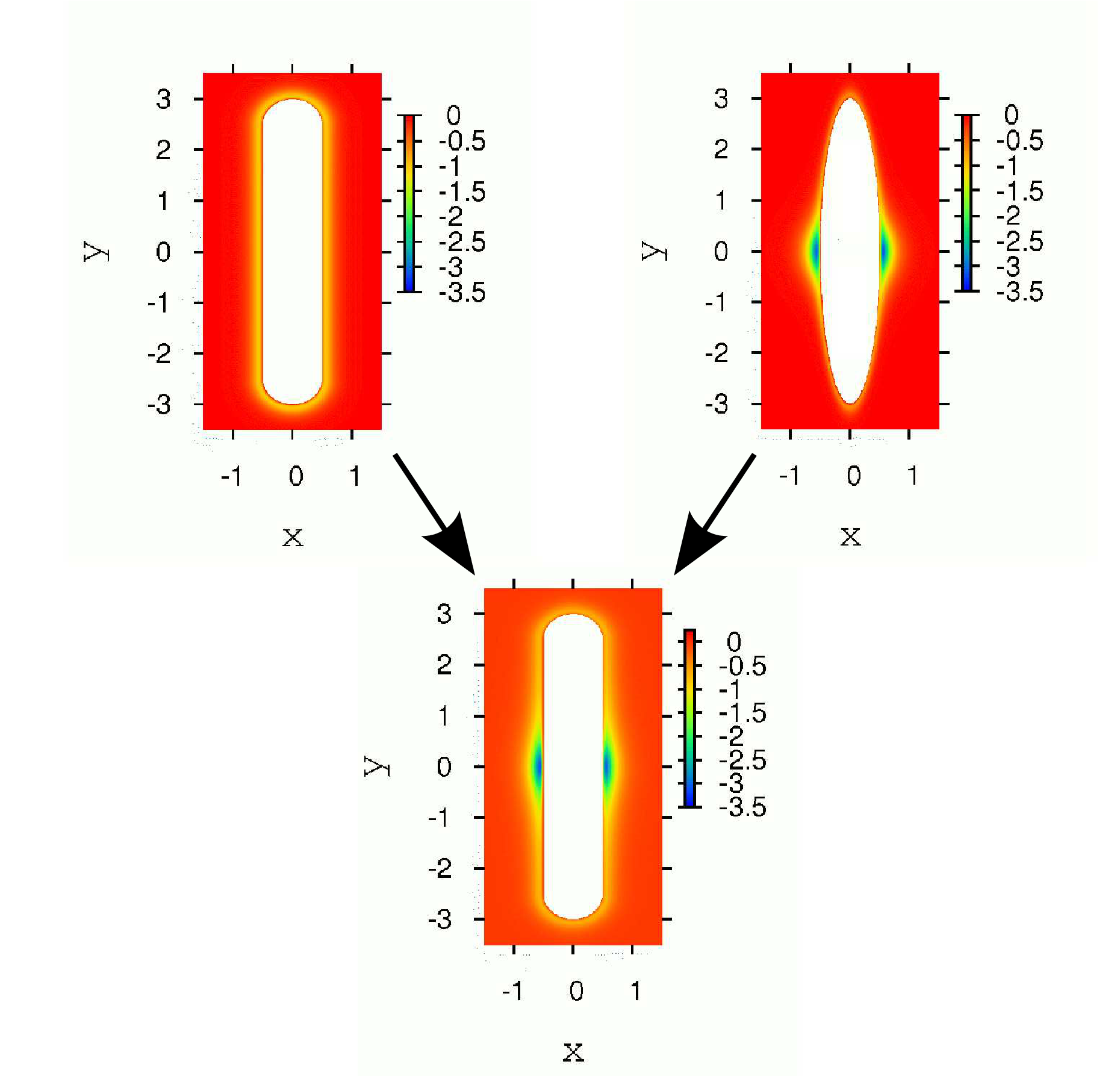
At this stage a couple of additional comments apply. For example, the reader may notice that Eqs. (7) and (8) are identical with those describing the orientation dependence of the interaction strength in the well-known Gay-Berne (GB) model of liquid crystals [30]. However, unlike in the GBK model a liquid crystal molecule is perceived as an ellipsoid of revolution in the GB model. This is effected by replacing the function $d_{ij}^{\mathrm{m}}(\bm{r}_{ij},\widehat{\bm{u}}_{i},\widehat{\bm{u}}_{j})$ in Eq. (6) by one that accounts properly for the shape of a molecule in the GB model [see, for example, Eq. (4) of Ref. 31]. The GBK model is also closely related to the so-called Kihara (K) model [32] of a liquid crystal [33]. In this latter model a molecule is again perceived as a spherocylinder but the interaction strength between a pair of molecules depends only on the minimum distance but not on the relative orientation of the molecules of a pair. This is achieved by setting $\kappa^{\prime}=1$ in Eq. (8b) such that $\varepsilon_{\mathrm{ff}}(\widehat{\bm{r}}_{ij},\widehat{\bm{u}}_{i},\widehat{\bm{u}}_{j})=\epsilon_{\mathrm{ff}}$ in Eq. (7). The shapes of molecules in the K, GB, and GBK models resulting from these manipulations are illustrated by the contour plots in Fig. 3.

The simulations (both MC and MD) to be presented below are based upon systems containing $N=1500$ molecules. Quantities of interest will be expressed in customary dimensionless (i.e., “reduced”) units. For example, length will be expressed in units of $\sigma$, energy in units of $\epsilon_{\mathrm{ff}}$, temperature in units of $\epsilon_{\mathrm{ff}}/k_{\mathrm{B}}$, time in units of $(\sigma^{2}m/\epsilon_{\mathrm{ff}})^{1/2}$ using $m=1$, and pressure $P_{\parallel}$ in units of $k_{\mathrm{B}}T/\sigma^{3}$ where $P_{\parallel}=\frac{1}{2}(P_{\mathrm{xx}}+P_{\mathrm{yy}})$ is related to diagonal components of the pressure tensor $\mathbf{P}$ acting in the $x$–$y$ plane.

We employ MC simulations in an isothermal-isobaric ensemble where we use $N$, $T$, $P_{\parallel}$, and $s_{\mathrm{z}0}$ as input parameters. In all the simulations we fix $s_{\mathrm{z}0}=19$ and consider $T=4.0$ and $6.0$. To reduce the computational cost interactions between fluid molecules are cut off beyond a minimum distance $d_{\mathrm{c}}^{\mathrm{m}}=3$. In addition, we employ a conventional Verlet neighborlist where molecules up to a minimum distance of $8$ are included as neighbors [34]. In the $x$- and $y$-directions periodic boundary conditions are applied.

In MC we employ the algorithm of Schoen [35] with one important modification. Rather than changing the area $A$ of the simulation box in the sense of a similarity transformation we allow the individual side lengths $s_{\alpha}$ ($\alpha=x$, $y$) to vary independently such that the shape of the simulation cell may change during the course of a simulation. This is important to preserve the in-plane isotropy of $\mathbf{P}$ especially in highly ordered N, smA, or RN phases. Our runs start from a sufficiently low pressure in the isotropic phase. In the initial configuration molecules are perfectly aligned and then allowed to relax to the isotropic state. The last configuration of this run is then used as a starting configuration of the next run at a slightly higher $P_{\parallel}$. We continue with such a compression sequence until the last state point of the highest pressure of interest has been reached. We refer to a MC step as $N$ attempted displacements or rotations and one attempted change of $s_{\alpha}$. Displacements and rotations as well as changes for $\alpha=x$ or $\alpha=y$ are performed with equal probability. Our runs are based upon $3\times 10^{5}$ equilibration steps followed by $2\times 10^{5}$ production steps for thermodynamic states sufficiently far away from any phase transition; around these transitions the number of production steps was enlarged to $7\times 10^{5}$. However, in changing $A$ as described care has to be taken that none of the instantaneous side lengths $s_{\alpha}$ becomes shorter than twice the neighbor-list cutoff given above.

MC simulations are mainly employed to generate suitable starting configurations for the subsequent MD simulations. In addition, MC is used to independently verify the correctness of the MD simulations through a comparison of equilibrium properties accessible to both types of simulations. In MD we employ the velocity Verlet algorithm for linear molecules in the implementation suggested by Ilnytskyi and Wilson [36]. The iterative solution of the equations of motion is initiated by using the last configuration of the MC simulation at the same state point as a starting configuration where velocities are taken at random from a Maxwell-Boltzmann distribution at the desired temperature. This starting configuration is equilibrated for another $10^{6}$ time steps of $\delta t=0.02$ using a simple velocity rescaling thermostat. The equilibrated system is then monitored for another $2\times 10^{7}$ time steps with no applied thermostat. During this part of the run the integration time step is reduced to $\delta t=10^{-4}$.

To characterize the structure of N, smA, and RN phases we begin by introducing suitably defined order parameters. For nematic phases this is accomplished via the so-called alignment tensor defined as [37]

where “$\otimes$” denotes the direct (i.e., dyadic) product and $\mathbf{1}$ is the unit tensor. Hence, $\mathbf{Q}$ is a real, symmetric, and traceless second-rank tensor which can be represented by a $3\times 3$ matrix. For a given configuration $(\bm{R},\widehat{\bm{U}})$, $\mathbf{Q}$ can be diagonalized in the basis of its three eigenvectors $\widehat{\bm{n}}_{-}$, $\widehat{\bm{n}}_{0}$, and $\widehat{\bm{n}}_{+}$ with associated eigenvalues $\lambda_{-}$, $\lambda_{0}$, and $\lambda_{+}$. Conventionally [38], one then defines the Maier-Saupe [39, 40] nematic order parameter $S=\left\langle\lambda_{+}\right\rangle$ where angular brackets denote an ensemble (MC) or time average (MD). On account of its definition, $S=0$ in the isotropic phase if the orientation of the molecules is perfectly random whereas $S=1$ if the molecules are perfectly aligned with the director $\widehat{\bm{n}}=\widehat{\bm{n}}_{+}$ in the nematic phase.

Even though the nematic phase is characterized by a substantial degree of orientational order the distribution of center-of-mass positions exhibits the typical short-range order characteristic of ordinary fluids where the typical correlation lengths are comparable to the range of intermolecular interactions. This changes in the smA phase where molecules do not only align with $\widehat{\bm{n}}$ but develop long-range positional order, that is they form individual layers in the direction of $\widehat{\bm{n}}$. However, positional order remains short-range in directions orthogonal to $\widehat{\bm{n}}$ such that within a given layer the structure remains fluid-like. Because of the layering of the fluid in the direction of $\widehat{\bm{n}}$ a suitable quantitative measure of smectic order is given by the leading coefficient of the Fourier transform of the local density $\rho(\bm{r}\cdot\widehat{\bm{n}})$

where $d$ is the spacing between adjacent smA layers. If these layers were ideal, $d=\kappa$ (see Sec. II.1). However, in practice $d\gtrsim\kappa$ on account of thermal fluctuations. Hence, in each configuration $(\bm{R},\widehat{\bm{U}})$, $d$ is adjusted such as to maximize $\Lambda$. From Eq. (12) it is also apparent that $\Lambda\in\left[0,1\right]$. In the nematic phase the superposition of the complex exponential functions in Eq. (12) causes $\Lambda\approx 0$ because in the direction of $\widehat{\bm{n}}$ a periodic structural feature of peridodicity $d$ does not exist; by a similar token $\Lambda\approx 1$ in the smA phase.

Plots of both $S$ and $\Lambda$ are presented in Fig. 4 for temperatures $T=4.0$ and $6.0$. As one can see from the plots, both $S$ and $\Lambda$ are small at low pressures indicating the presence of the I phase. Ideally, $S=0$ in the I phase but in practice attains small positive values of about $0.2$. This is partly due to the substrates which induce a certain degree of nematic order in those portions of the confined liquid crystal that are closest to either substrate. However, a nonvanishing value of $S$ in the isotropic phase is also due to a small but significant finite-size effect that is well-known and has been studied quantitatively in the literature [38, 41]. Here we adopt a value $S\simeq 0.4$ as a sensible heuristic definition of the threshold above which the N phase exists in agreement with the mean-field theory of Maier and Saupe [39, 40]. From Fig. 4 it therefore appears that the N phase forms somewhere above $P_{\parallel}\simeq 1.0$ ($T=4.0$) and $1.2$ ($T=6.0$), respectively.

Focusing on the lower temperature first, $S$ increases in the N phase with pressure up to $P_{\parallel}\simeq 1.7$ indicating the increase of nematic order. Over the same pressure range there are no smectic layers because $\Lambda\lesssim 0.2$ remains relatively small. However, at $P_{\parallel}\simeq 1.8$, smectic layers are forming as reflected by $\Lambda\simeq 0.8$. Simultaneously, $S$ keeps increasing as well because in the smA phase molecules align themselves even better with $\widehat{\bm{n}}$. The smA phase remains stable until $P_{\parallel}\simeq 2.2$ has been attained. Beyond this pressure $S$ remains nearly constant at a high value of about $1.0$ whereas $\Lambda$ drops rapidly until a residual small value of about $\Lambda\simeq 0.1$ is assumed which remains constant at all higher pressures considered. The drop in $\Lambda$ with $P_{\parallel}$ clearly reflects the disappearance of smectic layers present at lower $P_{\parallel}$. Because $S\simeq 1.0$ over the same pressure range we conclude that at sufficiently high pressures the structure of the confined fluid becomes nematic again in a reentrant fashion. To distinguish the high-pressure from the low-pressure nematic we refer to the former as RN because N and RN phases are seperated by an intermittent smA phase.

At $T=6.0$ these general features of the order-parameter plots in Fig. 4 prevail except that $\Lambda$ never rises above the residual value of about $0.1$. Hence, the smA phase does not form at this temperature. Nevertheless, we notice a small, step-like increase at $P_{\parallel}\simeq 2.2$ in the plot of $\Lambda$. At this and all larger pressures considered the nematic order is high and increases even further reflected by a monotonic increase of $S$ toward its limiting value $1.0$. For $P_{\parallel}\gtrsim 2.2$ the confined fluid exhibits structural features of the RN phase (see below). We shall therefore keep the acronym despite the missing intermittent smA phase.

To get a better feel for the structure of the confined fluid in the N, smA, and RN phases we present configuration “snapshots” from our simulations in Fig. 5. The plot in Fig. 5(a) illustrates the structure of the N phase: one clearly recognizes a preferred net orientation of the molecules but no significant positional order of the center-of-mass distribution. In Fig. 5(b) the layer structure characteristic of the smA phase is visible. These layers disappear in the RN phase as shown in Fig. 5(c). However, a large degree of orientational order is preserved as one realizes from this latter plot.

A more quantitative analysis of the structure of confined liquid crystals in the various ordered phases is enabled by plots of the local density

where $\delta\left(z-z_{i}\right)$ denotes the Dirac $\delta$-function, $N\left(z\right)$ is the number of molecules with their centers of mass located within a interval of width $\delta_{\mathrm{z}}=0.1$, and $A=s_{\mathrm{x}}s_{\mathrm{y}}$ is the instantaneous area of the simulation cell of side length $s_{\alpha}$ ($\alpha=\text{x, y}$) in the $\alpha$-direction. Hence, $\rho\left(z\right)$ is a measure of the probability of finding the center of mass at a specific position $z$. Plots in Fig. 6 illustrate the local structure of the confined liquid crystal in the direction of the substrate normal (i.e., perpendicular to the director $\widehat{\bm{n}}$). As is well-known from simple fluids [42], in confinement $\rho(z)$ is an oscillatory function of position sufficiently close to the substrate surfaces. The oscillations indicate that molecules arrange their centers of mass in individual layers parallel with the substrate. The location of a molecular layer is therefore indicated by a peak in $\rho\left(z\right)$. In the immediate vicinity of the solid substrate $\rho\left(z\right)\to 0$ because of the diverging fluid-substrate repulsion as $\left|z\right|\to s_{\mathrm{z}}/2$.

These general features may be seen from the plots in Fig. 6. One notices that in the N phase oscillations in $\rho\left(z\right)$ are restriczed to the immediate vicinity of the solid substrates [see Fig. 6(a)]. The oscillations decay exponentially as $\left|z\right|\to 0$ with a correlation length determined by bulk properties [43] whereas the spacing between neighboring layers reflects the molecular shape [44]. In the N phase a bulk-like region of considerable width exists in which $\rho\left(z\right)$ is constant as the plot in Fig. 6(a) reveals. On the contrary, layering is much more pronounced in the smA phase as a comparison of plots in Figs. 6(a) and 6(b) indicates: Peaks in Fig. 6(b) are taller and because a bulk-like region is absent the entire confined fluid is organized in layers. However, the layered structure becomes weaker as one approaches the center of the slit pore as reflected by the decay of $\rho\left(z\right)$ in Fig. 6(b). Finally, in the RN phase layering is even more pronounced as the plot in Fig. 6(c) shows. Moreover, plots in Fig. 6(b) and 6(c) reveal another subtle structural change. Counting maxima in the plots of $\rho\left(z\right)$ one realizes that one additional layer of molecules is present in the RN compared with the smA phase. The presence of this additional layer points to a more efficient packing of molecules as far as the arrangement of their centers of mass is concerned. A more efficient packing becomes possible because the layered structure characteristic of the smA phase [see Fig. 5(b)] is lost in the RN phase [see Fig. 5(c)].

Next, at $T=6$ one realizes from Fig. 7 a similar formation of an additional molecular layer but without occurrence of an intermittent smectic phase. Plots in Figs. 7(a) show that for two state points in the nematic phase an increase in pressure only causes the layers already present to become more distinct. For example, $\rho\left(z\right)$ drops to zero in regions between individual layers at the higher pressure whereas $\rho\left(z\right)$ remains nonzero over the corresponding ranges at the lower pressure. The plot in Fig. 7(b) corresponds to a state point where the confined fluid undergoes the subtle reorganization that will eventually lead to the growth of an additional layer. As one approaches the midplane located at $z=0$ individual peaks in $\rho\left(z\right)$ first broaden and eventually split up into two unresolved peaks. At an even higher pressure considered in Fig. 7(c) we realize that the fluid has completed its structural reorganization and a new fluid layer emerges as we can see by comparing this plot with its counterparts shown in Fig. 7(a). Moreover, visual inspection of a characteristic configuration [see Fig. 5(c)] reveals that in the RN phase molecules appear in string-like arrangements.

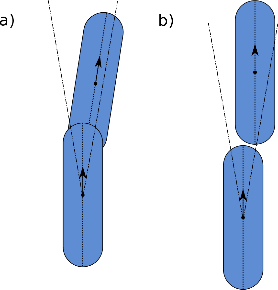
In our terminology a “string” is a sequence of molecules arranged in space like individual cars of a train with their long axes all pointing in the same direction. The “snapshot” of a typical configuration presented in Fig. 5(c) already indicates that these supramolecular strings are omnipresent in the RN phase. In mathematical terms an ideal string can therefore be defined through the relations

where, of course, one of the two scalar products in Eq. (14b) is redundant. In practice, however, small deviations from perfect alignment of molecules in a string arise on account of thermal fluctuations. A good measure of the extent to which a pair of molecules is arranged in a string-like conformation approximately may be defined by decomposing the distance vector $\bm{r}_{ij}$ between the centers of mass of nearest-neighbor molecules $i$ and $j$ into components parallel and perpendicular to $\widehat{\bm{u}}_{i}$ through the expressions (see Fig. 1)

For a string-like configuration of a pair of molecules one anticipates $r_{ij}^{\perp}\equiv\left|\bm{r}_{ij}^{\perp}\right|\to 0$. However, a second characteristic conformation characterized by relatively small values of $r_{ij}^{\perp}$ is conceivable. In this conformation molecules are arranged in a shifted side-side arrangement [see Fig. 8(a)]. Plots of configurational snapshots in Fig. 5 clearly show that also unshifted side-side arrangements exist both in the N and in the RN phase. This is because they are energetically favored according to Fig. 3(a). However, they are also present to some extent in other phases as snapshots in Figs. 5(a) and 5(c) indicate. To eliminate these unwanted unshifted side-side conformations in favor of only shifted ones it is prudent from an operational point of view to consider only the subset $\left\{\widetilde{\bm{r}}_{ij}^{\perp}\right\}\subseteq\left\{\bm{r}_{ij}^{\perp}\right\}$ defined through

where we arbitrarily take $\delta_{\kappa}=0.2$ and $\delta_{\cos\theta}=0.98$. To see that this rather complex definition selects only those conformations sketched in Figs. 8(a) and 8(b) one needs to realize that the first of the three conditions in Eq. (16) selects nearest neighbors $\{j\}$ of a given molecule $i$, the second condition favors head-tail-like conformations, whereas the third one selects molecules with nearly perfectly aligned long molecular axes. It is then convenient to introduce the probability

for a quantitative discussion of the formation of string-like structures where $\mathcal{P}_{0}$ is a normalization constant which we determine via

In the actual simulations we obtain $\mathcal{P}(r^{\perp})$ as a histogram using $\delta r^{\perp}=0.02$ as the bin width.

Plots in Fig. 9 show $\mathcal{P}(r^{\perp})$ for different temperatures and pressures in the I, N, smA, and RN phase. At sufficiently low pressures it is evident from the insets in Figs. 9(a) and 9(b) that $\mathcal{P}(r^{\perp})$ increases monotonically with $r^{\perp}$ and reaches a broad maximum located approximately at $r^{\perp}\simeq 1.25$ irrespective of whether the I, N, or smA phase is considered. That $\mathcal{P}(r^{\perp})$ rises with $r^{\perp}$ may be ascribed to molecules in the I, N, and smA phase that arrange their long axes locally to a certain degree. This local order is solely caused by the intermolecular interaction potential which favors local side-side conformations of molecules [see Fig. 3(a)].

In the RN phase the form of $\mathcal{P}(r^{\perp})$ is completely different. Here the plots in Fig. 9(a) and 9(b) exhibit two maxima. The largest one slightly above $r^{\perp}\simeq 1.0$ corresponds to conformations in which neighboring particles are arranged in the shifted side-side conformation depicted schematically in Fig. 8(a). Note that these values of $r^{\perp}$ are slightly below the position of the minimum of the interaction potential (see Fig. 2). The secondary maximum of $\mathcal{P}(r^{\perp})$ in the RN phase at $r^{\perp}<0.5$ corresponds to string-like conformations schematically illustrated by the plot in Fig. 8(b). Were the string-like conformation perfect one would anticipate a peak of $\mathcal{P}(r^{\perp})$ at $r^{\perp}=0$. However, on account of thermal fluctuations these ideal string-like conformations are only infrequently observed. For example, closer scrutiny would reveal that $\mathcal{P}(r^{\perp})\neq 0$ at $r^{\perp}=0$ indicating that a very small fraction of molecules does, in fact, assume an ideal string-like conformation. As $P_{\parallel}$ increases one notices that both peaks of $\mathcal{P}(r^{\perp})$ shift to progressively smaller $r^{\perp}$. This fact reflects an arrangement of molecules in more perfect string-like conformations with increasing pressure as one would expect intuitively.

One also notices from plots in Figs. 9(a) and 9(b) that the curves seem to intersect in isolated points at characteristic values of $r^{\perp}$. These intersections may be interpreted as “isosbestic” points (derived from the Greek words isos: equal, the same and sbestos: extinguishable) [45], a concept widely known in spectroscopy. The occurrence of isosbestic points is relatively simple to grasp. We assume that $\mathcal{P}(r^{\perp})$ can be decomposed into a sum of three contributions:

1. 1.

   a probability distribution centered at $r^{\perp}\approx 1.0$ corresponding to a population of shifted side-side molecular conformations [see Fig. 8(a)],

2. 2.

   a probability distribution centered at $r^{\perp}\approx 0.25$ corresponding to a population of shifted string-like molecular conformations [see Fig. 8(b)],

3. 3.

   and a probability distribution representing all other molecular conformations satisfying Eq. (16) and embracing the entire range of $r^{\perp}$.

For sufficiently large $P_{\parallel}$ the distributions of 1 and 2 can be assumed to be well separated whereas 3 may be thought of as a broad background distribution. Intersections between distributions 1 and 3 or between 2 and 3, respectively, will give rise to isosbestic points. As $P_{\parallel}$ increases distributions 1 and 2 become sharper and increase in height at the expense of the background distribution 3; furthermore, maxima of both distributions 1 and 2 shift to lower values of $r^{\perp}$ indicating an increase in order. Importantly, the emergence of two well-defined peaks in $\mathcal{P}(r^{\perp})$ is a fingerprint of the RN phase and could therefore be taken as computational evidence to detect RN phases even though its experimental significance may be limited. Incidentally, at low $P_{\parallel}$ (i.e., in the I, N, or smA phase) the only important distributions are 1 and 2 because string-like conformations are statistically irrelevant. Consequently, only one isosbestic point exists as shown in the insets of Fig. 9.

The formation of string-like conformations has important ramifications as far as dynamic properties of the RN phase are concerned. To illustrate this we begin by considering a persistence probability

defined as the correlation function of the angle between a pair of molecules $(i,j)$ which at the initial time $t$ satisfy the conditions for a string-like conformation introduced in Eq. (16). Subscript “$t$” is attached to the angular brackets to emphasize that averaging involves a sufficiently large number of statistically uncorrelated time origins which implicitly invokes the principle of stationarity of temporal correlation functions in equilibrium systems [46]. In Eq. (19) $\eta_{ij}\equiv\widehat{\bm{u}}_{i}\cdot\widehat{\bm{r}}_{ij}$ is the cosine of the angle between the instantaneous orientation of a reference molecule $i$ and the unit vector connecting its center of mass to that of another molecule $j$ as time passes [see Fig. 1]. Because of this definition, $\eta_{ij}\left(t+\tau\right)$ is a measure of the relative orientation of a molecular pair at time $t+\tau$ given that its orientation at time $t$ is $\eta_{ij}\left(t\right)$. Therefore, $\sigma\left(\tau\right)\to 1$ as $\tau\to 0$ in agreement with plots in Figs. 10(a) and 10(b) for various temperatures and pressures. At sufficiently low $P_{\parallel}$, $\sigma\left(\tau\right)$ eventually decays with increasing time. The decay is delayed the more as the nature of the liquid-crystalline phase changes in the direction I$\to$N$\to$smA, that is with increasing $P_{\parallel}$ [see Fig. 10(a)].

One also notices from Fig. 10(a) that the decorrelation of relative orientations becomes very slow as soon as one enters the RN phase. This is already evident from the plot for $P_{\parallel}=2.3$ immediately after the smA-RN phase transition has occurred (see Fig. 4). However, the corresponding plot in Fig. 10(a) shows that $\sigma(\tau)$ eventually decays at long times. This is apparently not so at the higher pressure $P_{\parallel}=2.8$ in the RN phase. The relevant plot in Fig. 10(a) shows only a weak decay of $\sigma\left(\tau\right)$ over an intermediate time range $1\lesssim\tau\lesssim 10$ and then remains nearly constant for longer times $\tau>10^{3}$. The shape of $\sigma\left(\tau\right)$ seems to reflect a two-stage decorrelation process involving those conformations represented by the bimodal distribution $\mathcal{P}(r^{\perp})$ plotted in Fig. 9(a). In fact, intuitively it seems sensible to assume that decorrelation during the intermediate time interval is associated with the orientational dynamics of shifted side-side conformations depicted in Fig. 8(a). These conformations are expected to be less stable than the string-like ones depicted in Fig. 8(b). This notion is further corroborated by the slowing down of the dynamics at longer times with increasing $P_{\parallel}$ which causes the population of string-like conformations to increase according to plots in Figs. 9. This qualitative picture remains unaltered at the higher $T=6.0$ as parallel plots in Fig. 10(b) show. However, at this temperature the smA phase is absent in agreement with our earlier analysis of various structural quantities.

From the discussion of orientational relaxation one may get the impression that the RN phase is rather sluggish with respect to its dynamics. While this is certainly true for the rotational dynamics it turns out that mass transport is actually quite fast in the RN phase. A suitable measure of mass transport is the mean square displacement (MSD) of molecules. It measures the on-average net distance a molecule’s center of mass is able to travel in a given amount of time. Because of the large degree of nematic order characteristic of the RN phase it seems sensible to introduce a specialized MSD by considering displacements of molecules in the direction of their long axes. Specifically, we define $\bm{r}_{i}^{\parallel}\equiv\widehat{\bm{u}}_{i}\cdot\bm{r}_{i}$ such that the associated MSD for the displacement of molecules in the direction of their long axes may be cast as

Plots in Fig. 11 illustrate the variation of the MSD with time on a double-logarithmic scale. At short times $\tau\leq 10^{-1}$ MSDs for various phases collapse onto a single curve. In this regime, known as the ballistic regime, the MSD increases proportionally to $\tau^{2}$. In the ballistic regime molecules travel freely, that is for sufficiently short times interactions with neighboring molecules are inconsequential. As a consequence, the specific nature of the phase under study does not matter such that the MSDs for different phases become indistinguishable and can be represented by a unique curve.

At sufficiently long times, however, the motion of molecules becomes diffusive, that is $\left\langle\Delta r_{\parallel}^{2}\left(\tau\right)\right\rangle_{t}\propto\tau$. In the diffusive regime intermolecular interactions do, of course, matter greatly unlike in the ballistic regime. Therefore, in the diffusive regime plots in Figs. 11(a) and 11(b) cannot be represented by a single curve but differ between I, N, smA, and RN phases. An inspection of the MSD for the smA phase reveals that ballistic and diffusive regimes are separated by a third, subdiffusive regime in which $\left\langle\Delta r_{\parallel}^{2}\left(\tau\right)\right\rangle_{t}\propto\tau^{\alpha(\tau)}$ where $1\lesssim\alpha(\tau)\lesssim 2$ varies continuously. The crossover region of subdiffusive behavior reflects the presence of smectic layers because $\left\langle\Delta r_{\parallel}^{2}\left(\tau\right)\right\rangle_{t}$ is a measure for mass transport in a direction normal to the layer plane [see Fig. 5(b)]. Diffusive motion of molecules out of their original smectic layer into a neighboring one is inhibited by the compactness of the layered structure. However, within each layer there is sufficiently little order such that molecules may eventually move from their original to a neighboring layer. This process demarcates the onset of ordinary diffusive motion. Depending on the local compactness of the smectic layers it may take some molecules longer than others before they exhibit diffusive motion and this is the reason why the subdiffusive regime is characterized by a constant change in the time dependence of the MSD characterized by the exponent $\alpha(\tau)$.

As a quantitative measure of mass transport in the diffusive regime it is convenient to introduce the self-diffusion coefficient $D_{\parallel}$ via the expression

which corresponds to the long-time slope of the MSDs plotted in Figs. 11. From that definition and the plots in Figs. 11 one immediately anticipates a self-diffusion constant which is largest in the RN phase compared with the other three phases. In fact, the plot in Fig. 12 shows a dramatic increase of $D_{\parallel}$ as one enters the RN phase whereas lower-pressure (I, N, or smA) phases exhibit rather small self-diffusivity. In particular, the smA phase is characterized by nearly vanishing self-diffusion constants which can be rationalized as above where we argued that the relatively compact layered structure makes it difficult for molecules to diffuse out of their original layer and penetrate into a neighboring one. The dramatic increase in mass transport in the direction of $\widehat{\bm{n}}$ in combination with nearly perfect nematic order prompted us to refer to liquid crystals in the RN phase as “supernematics” [21].

More detailed insight into the dynamics of mass transport in the RN phase can be gained by also considering the MSD for molecular displacements in the direction orthogonal to the molecules’ long axes [47] to which we refer as $\left\langle\Delta r_{\perp}^{2}\left(\tau\right)\right\rangle_{t}$ by analogy with Eq. (20) where, of course, we replace $\bm{r}_{i}^{\parallel}$ by its counterpart $\bm{r}_{i}^{\perp}\equiv\bm{r}_{i}-(\widehat{\bm{u}}_{i}\cdot\bm{r}_{i})\widehat{\bm{u}}_{i}$. Plots of the root MSD’s for perpendicular versus parallel molecular displacements $\Delta\overline{r}_{\perp,\parallel}\equiv\sqrt{\left\langle\Delta r_{\perp,\parallel}^{2}\left(\tau\right)\right\rangle_{t}}$ in Fig. 13 reveal that dynamically distinct regimes exist. In the ballistic regime the plot in Fig. 13 increases linearly with slope $1$ which can be rationalized as follows. Over the relatively short times characteristic of the ballistic regime molecules move freely in space. Hence, their self-diffusion is largely controlled by the free volume surrounding a molecule. In the RN phase the shape of the free volume should be closely related to the shape of an individual spherocylinder. Therefore, rescaling $\Delta\overline{r}_{\parallel}\left(\tau\right)$ by the aspect ratio $\kappa$ and expressing $\Delta\overline{r}_{\perp}\left(\tau\right)$ in units of $\sigma$ one anticipates the plot in Fig. 13 to increase linearly with a slope of $1$ in the ballistic regime where both $\Delta\overline{r}_{\perp}\left(\tau\right)$ and $\Delta\overline{r}_{\parallel}\left(\tau\right)$ are small compared with $\sigma$. If this condition does not hold any longer intermolecular interactions begin to matter and self-diffusion is no longer ballistic. The plot in Fig. 13 shows that during the initial stage of non-ballistic self-diffusion the plot of $\Delta\overline{r}_{\perp}\left(\tau\right)$ versus $\Delta\overline{r}_{\parallel}\left(\tau\right)$ levels off and reaches a plateau. During this stage molecules diffuse in string-like conformations which remain intact, that is the group of molecules forming a string-like conformation stays together as an entity. However, if both $\Delta\overline{r}_{\perp}\left(\tau\right)$ and $\Delta\overline{r}_{\parallel}\left(\tau\right)$ are sufficiently larger than $\sigma$ the plot in Fig. 13 increases again linearly but with a somewhat smaller slope of about $0.88$ compared with the initial ballistic regime. Because in this second linear regime $\Delta\overline{r}_{\perp}\left(\tau\right)$ is of the order of several $\sigma$, diffusive motion must involve the exchange of individual molecular units between neighboring supramolecular “strings” which illustrates the complexity of the dynamics in the supernematic RN phase.

References

- [1] H. Kleinert, S. Schmidt, and A. Pelster, Phys. Rev. Lett. 93, 160402 (2004).
- [2] C. Bechinger, Q.-H. Wei, and P. Leiderer, J. Phys.: Condens. Matter 12, A425 (2000).
- [3] M. B. Pinto, R. O. Ramos, and J. E. Parreira, Phys. Rev. D 71, 123519 (2005).
- [4] N. Osaka, S. Miyazaki, S. Okabe, H. Endo, A. Sasai, K.-I. Seno, S. Aoshima, and M. Shibayama, J. Chem. Phys. 127, 094905 (2007).
- [5] J. Dudowicz, J. F. Douglas, and K. F. Freed, J. Chem. Phys. 130, 164905 (2009).
- [6] S. M. M. Ramos, A. Benyagoub, B. Canut, and C. Jamois, Langmuir 26, 5141 (2010).
- [7] J. Szydlowska, A. Krówczyński, R. Bilewicz, D. Pociecha, and Ł. Głaz, J. Mater. Chem 18, 1108 (2008).
- [8] P. E. Cladis, Phys. Rev. Lett. 35, 48 (1975).
- [9] W. K. Lee, B. A. Wintner, E. Fontes, P. A. Heiney, M. Ohba, J. N. Haseltine, and A. B. Smith, Liq. Cryst. 4, 87 (1989).
- [10] D. Pociecha, E. Gorecka, and M. Čepič, Phys. Rev. Lett. 86, 3048 (2001).
- [11] G. Heppke, H.-S. Kitzerow, D. Lötzsch, and C. Papenfuß, Liq. Cryst. 8, 407 (1990).
- [12] G. Sigaud, N. Huu Tinh, F. Hardouin, and H. Gasparoux, Mol. Cryst. Liq. Cryst. 69, 81 (1981).
- [13] P. E. Cladis, R. K. Bogardus, W. B. Daniels, and G. Taylor, Phys. Rev. Lett. 39, 720 (1977).
- [14] F. Hardouin, G. Sigaud, M. F. Archard, and H. Gasparoux, Phys. Lett. A 71, 347 (1979).
- [15] P. E. Cladis, Mol. Cryst. Liq. Cryst. 165, 85 (1988).
- [16] L. Longa and W. H. de Jeu, Phys. Rev. A 26, 1632 (1982).
- [17] A. N. Berker and J. S. Walker, Phys. Rev. Lett. 47, 1469 (1981).
- [18] R. R. Netz and A. N. Berker, Phys. Rev. Lett. 68, 333 (1992).
- [19] A. Ferrarini, G. R. Luckhurst, P. L. Nordio, and E. Spoalore, Mol. Phys. 89, 1087 (1996).
- [20] E. de Miguel and E. M. del Río, Phys. Rev. Lett. 95, 217802 (2005).
- [21] M. G. Mazza, M. Greschek, R. Valiullin, J. Kärger, and M. Schoen, Phys. Rev. Lett. 105, 227802 (2010).
- [22] B. J. Borah, H. Jobic, and S. Yashonath, J. Chem. Phys. 132, 144507 (2010).
- [23] R. Y. Dong, J. Chem. Phys. 75, 2621 (1981).
- [24] R. Y. Dong, J. Chem. Phys. 76, 5659 (1982).
- [25] S. Miyajima, K. Akaba, and T. Chiba, Solid State Commun. 49, 675 (1984).
- [26] J. Bharatam and C. R. Bowers, J. Phys. Chem. B 103, 2510 (1999).
- [27] F. Vollrath and D. P. Knight, Nature 410, 541 (2001).
- [28] B. Martínez-Haya, A.Cuetos, S. Lago, and L. F. Rull, J. Chem. Phys. 122, 024908 (2004).
- [29] C. Vega and S. Lago, Comput. Chem. 18, 55 (1994).
- [30] J. G. Gay and B. J. Berne, J. Chem. Phys. 74, 3316 (1981).
- [31] T. Gruhn and M. Schoen, Phys. Rev. E 55, 2861 (1997).
- [32] T. Kihara, Adv. Chem. Phys. 5, 147 (1963).
- [33] A. Cuertos, B. Martínez-Haya, S. Lago, and L. F. Rull, Phys. Rev. E 68, 011704 (2003).
- [34] L. Verlet, Phys. Rev. 159, 98 (1967).
- [35] M. Schoen, Physica A 270, 353 (1999).
- [36] J. M. Ilnytskyi and M. R. Wilson, Comput. Phys. Commun. 148, 43 (2002).
- [37] H. Pardowitz and S. Hess, Physica A 100, 540 (1980).
- [38] R. Eppenga and D. Frenkel, Mol. Phys. 52, 1303 (1984).
- [39] W. Maier and A. Saupe, Z. Naturforsch 14a, 882 (1959).
- [40] W. Maier and A. Saupe, Z. Naturforsch. 15a, 287 (1960).
- [41] A. Richter and T. Gruhn, J. Chem. Phys. 125, 064908 (2006).
- [42] M. Schoen and S. H. L. Klapp, Nanoconfined Fluids. Soft Matter Between Two and Three Dimensions (Wiley-VCH, 2007).
- [43] S. H. L. Klapp, Y. Zeng, D. Qu, and R. v. Klitzing, Phys. Rev. Lett. 100, 118303 (2008).
- [44] M. Greschek, M. Melle, and M. Schoen, Soft Matter 6, 1898 (2010).
- [45] G. W. Robinson, C. H. Cho, and J. Urquidi, J. Chem. Phys. 111, 698 (1999).
- [46] J. P. Hansen and I. R. McDonald, Theory of Simple Liquids (Academic Press, 2006).
- [47] H. Löwen, Phys. Rev. E 59, 1989 (1999).
- [48] M. Karplus and J. N. Kushick, Macromolecules 14, 325 (1981).
- [49] L. D. Landau and E. M. Lifshitz, Statistical Physics (Pergamon Press, London, 1980).
- [50] Y.-C. Liu, J. D. Moore, Q. Chen, T. J. Roussel, Q. Wang, and K. E. Gubbins, “Diffusion fundamentals, vol. 3,” (Leipziger Universitätsverlag, Leipzig, 2009) p. 164.
- [51] V. Kukla, J. Kornatowski, D. Demuth, I. Girnus, H. Pfeifer, L. V. C. Rees, S. Schunk, K. K. Unger, and J. Kärger, Science 272, 702 (1996).
- [52] T. Kaneko, Y. F. Li, S. Nishigaki, and R. Hatakeyama, J. Am. Chem. Soc. 130, 2714 (2008).
- [53] C. Lutz, M. Kollman, and C. Bechinger, Phys. Rev. Lett. 93, 026001 (2004).
- [54] R. Valiullin, J. Kärger, and R. Glaser, Phys. Chem. Chem. Phys. 11, 2833 (2009).
- [55] S. V. Dvinskikh and I. Furo, J. Chem. Phys. 115, 1946 (2001).
- [56] R. Valiullin and A. Khokhlov, Phys. Rev. E 73, 051605 (2006).
- [57] W. E. Maas, F. H. Laukien, and D. G. Cory, J. Am. Chem. Soc. 118, 13085 (1996).
- [58] E. E. Romanova, F. Grinberg, A. Pampel, J. Kärger, and D. Freude, J. Magn. Res. 196, 110 (2009).
- [59] D. Fincham, Mol. Simul. 11, 79 (1993).