∎

Multidimensional Quasi-Monte Carlo Malliavin Greeks

Nicola Cufaro Petroni
Dipartimento di Matematica and TIRES Università di Bari
INFN Sezione di Bari
via E. Orabona 4 70125 Bari Italy
email: cufaro@ba.infn.it

Piergiacomo Sabino
Dipartimento di Matematica Università di Bari
via E. Orabona 4 70125 Bari Italy
email: sabino@dm.uniba.it

Abstract

We investigate the use of Malliavin calculus in order to calculate the Greeks of multidimensional complex path-dependent options by simulation. For this purpose, we extend the formulas employed by Montero and Kohatsu-Higa to the multidimensional case. The multidimensional setting shows the convenience of the Malliavin Calculus approach over different techniques that have been previously proposed. Indeed, these techniques may be computationally expensive and do not provide flexibility for variance reduction. In contrast, the Malliavin approach exhibits a higher flexibility by providing a class of functions that return the same expected value (the Greek) with different accuracies. This versatility for variance reduction is not possible without the use of the generalized integral by part formula of Malliavin Calculus. In the multidimensional context, we find convenient formulas that permit to improve the localization technique, introduced in Fournié et al and reduce both the computational cost and the variance. Moreover, we show that the parameters employed for variance reduction can be obtained on the flight in the simulation. We illustrate the efficiency of the proposed procedures, coupled with the enhanced version of Quasi-Monte Carlo simulations as discussed in Sabino, for the numerical estimation of the Deltas of call, digital Asian-style and Exotic basket options with a fixed and a floating strike price in a multidimensional Black-Scholes market.

Key Words: Greeks, Risk-Management, Quasi-Monte Carlo Methods, Malliavin Calculus.

1 Introduction and Motivation

Risk-sensitivities, also called Greeks, are fundamental quantities for the risk-management. Greeks measure the sensitivities of a portfolio of financial instruments with respect to the parameters of the underlying model. Mathematically speaking, a greek is the derivative of a financial quantity with respect to (w.r.t.) any of the parameters of the problem. As these quantities measure risk, it is important to calculate them quickly and with a small order of error. In general, the computational effort required for an accurate calculation of sensitivities is often substantially greater than that required for price estimation.

The problem of greeks calculation can be casted as follows. Suppose that the financial quantity of interest is described by $\mathbb{E}\left[\psi\left(X(\alpha)\right)Y\right]$ (i.e., the price of a derivative contract), where $\psi:\mathbb{R}\rightarrow\mathbb{R}$ is a measurable function and $X$ and $Y$ are two random variables (r.v.s). The greek, that we denote $\theta$ , is the derivative w.r.t. the parameter $\alpha$ :

\theta(\alpha)=\frac{\partial}{\partial\alpha}\mathbb{E}\left[\psi\left(X(\alpha)\right)Y\right]=\mathbb{E}\left[\frac{\partial}{\partial\alpha}\psi\left(X(\alpha)\right)Y\right].

The most common of the Greeks are notably, Delta, Gamma, Vega, Theta, Rho. These quantities are relatively simple to calculate for plain vanilla contracts in the Black-Scholes (BS) market. However, their evaluation is a complex and demanding task for exotic derivative contracts such as Asian-style basket options where no closed-formula is known.

The simplest and crudest approach is to employ the Monte Carlo (MC) estimation of $\mathbb{E}\left[\psi\left(X(\alpha)\right)Y\right]$ for two or more values of $\alpha$ and then use finite-difference approximations. However, this approach can be computationally intensive and can produce large biases and large variances in particular if $\psi=1\!\!1_{A}$ , where $A$ is a measurable set. A variant is the kernel method (see Montero and Kohatsu-Higa [10]) which generalizes finite-difference methods using ideas taken from the kernel density estimation.

Several alternatives have been proposed without finite-difference approximation. Pathwise methods (see Glasserman [4]) treat the parameter of differentiation $\alpha$ as a parameter of the evolution of the underlying model and differentiate this evolution. However, this approach is not always applicable, notably when $\psi$ is not smooth (for instance $\psi=1\!\!1_{A}$ ). At the other extreme, the likelihood method ratio (see Glasserman [4]) puts the parameter in the measure describing the underlying model and differentiates this measure. Even if the likelihood method ratio is applicable to non-smooth functions it may provide high-variance estimators. Indeed, compared to the pathwise method (when applicable), it displays a higher variance. Summarizing, these two alternatives involve two main ideas: differentiating the evolution or differentiating the measure, respectively.

In this paper we investigate the use of Malliavin Calculus in order to employ (Quasi)-Monte Carlo (QMC) simulations for the evaluation of the sensitivities of complex multidimensional path-dependent options. The multidimensional setting shows the very convenience of the Malliavin Calculus approach over the different techniques that have been proposed. Indeed, Malliavin Calculus allows to calculate sensitivities as expected values whose estimation is a natural application of MC methods. Formally:

\theta(\alpha)=\mathbb{E}\left[\frac{\partial}{\partial\alpha}\psi\left(X(\alpha)\right)Y\right]=\mathbb{E}\left[\psi\left(X(\alpha)\right)H\right].

where $H$ is a r.v. depending on $X$ and $Y$ .

In the context of multidimensional options, we extend the formulas employed by Montero and Kohatsu-Higa [11] to the multidimensional case. This approach gives a certain flexibility and provides a class of functions (different r.v.s $H$ ) returning the same expected value (the sensitivity) but with different accuracies.

Indeed, the previously mentioned alternative techniques may be computationally expensive in the multidimensional case and do not provide flexibility for variance reduction. This versatility for variance reduction is not possible without the use of the generalized integral by part formula of Malliavin Calculus. Advanced techniques such as the kernel density estimation or more recent approaches such as the Vibrato Monte Carlo in Gilles [3] are difficult to employ and computationally demanding in multi-dimensions. In order to avoid to use the Malliavin technique, Chen and Glasserman [1] have illustrated a procedure that produces “Malliavin Greeks” without Malliavin Calculus. However, since this procedure involves both pathwise and likelihood ratio methods, the estimators of the formulas for the sensitivities in Chen and Glasserman [1] have a high variance.

For these purposes we find convenient representations of $H$ that permit to enhance the localization technique introduced in Fournié et al. [2] and reduce both the computational cost and the variance. Moreover, we show that the parameters employed for the variance reduction can be obtained on the flight in the simulation by adaptive techniques. We illustrate the efficiency of the proposed procedures, coupled with the enhanced version of QMC simulations discussed in Sabino [16], for the numerical estimation of the Deltas of call, digital Asian-style and Exotic basket options with a fixed and a floating strike price in a multidimensional BS market.

The paper is organized as follows. Section 2 is a short introduction on Malliavin Calculus, Section 3 derives the formulas employed for the computation of the Deltas of call Asian basket options with floating and fixed strike, Asian digital options and exotic options. Section 4 illustrates the enhanced QMC approach that we adopt and describes in details how to get the localization parameters with adaptive (Q)MC techniques; Section 5 discusses the numerical experiments of the study and finally Section 6 summarizes the most important results and concludes the paper.

2 Malliavin Calculus: Basic Results and Notation

The aim of this section is to briefly introduce the basic results from Malliavin Calculus and to fix the notation we adopt in the rest of the paper. For more information on this subject, we refer the reader to the book by Nualart [13].

Consider the probability space $\left(\Omega,\mathcal{F},\mathbb{P}\right)$ where we define the $M$ -dimensional Brownian motion $\mathbf{W}(t)=\left(W_{1}(t),\dots,W_{M}(t)\right)$ , $t\in[0,T]$ and given $0=t_{0}^{(n)},t_{1}^{(n)},\dots,t_{n}^{(n)}$ , divide the interval $[0,T]$ into $n$ subintervals $I_{k}=[t_{k}^{(n)},t_{k+1}^{(n)})$ , $k=0,\dots,n-1$ . The superscripts indicates the fineness of the subdivision of $[0,T]$ . Now denote the vector $\Delta^{(n)}_{k}=\left(\Delta^{(n)}_{k,1},\dots,\Delta^{(n)}_{k,M}\right)$ where $\Delta^{(n)}_{k,i}=W_{i}(t_{k+1}^{(n)})-W_{i}(t_{k}^{(n)})$ .

Now consider a smooth function with polynomial growth $\phi:\mathbb{R}^{n\times M}\rightarrow\mathbb{R}$ , $\phi\in\mathcal{C}_{p}^{\infty}$ , of the form $\phi=\phi(\Delta^{(n)}_{0},\dots,\Delta^{(n)}_{n-1})$ . Finally we consider the following space:

\mathcal{S}_{n}=\left\{\phi(\Delta^{(n)}_{0},\dots,\Delta^{(n)}_{n-1});\phi\in\mathcal{C}_{p}^{\infty}\right\}\subset\mathcal{L}^{2}\left(\Omega\right),

(1)

where $\left(\mathcal{S}_{n}\right)_{n\geq 1}$ form an increasing sequence in $\mathcal{L}^{2}\left(\Omega\right)$ .

Definition 1

The union $\mathcal{S}=\left(\bigcup_{n\geq 1}\mathcal{S}_{n}\right)\subset\mathcal{L}^{2}\left(\Omega\right)$ is called simple functional space and its elements are called simple functionals.

We now can define the Malliavin derivative operator.

Definition 2

Let $\phi\in\mathcal{S}$ , then there exists $n\in\mathbb{N}^{*}$ such that $\phi=\phi(\Delta^{(n)})$ . The Malliavin derivative operator $\mathbf{D}=\left(D^{1},\dots,D^{M}\right)$ of $\phi$ at a point $s\in I_{k}$ is defined as

D_{s}^{m}\phi=\sum_{k=0}^{n-1}\frac{\partial\phi}{\partial x_{k,m}}(\Delta^{(n)}_{0},\dots,\Delta^{(n)}_{n-1})1\!\!1_{I_{k}^{(n)}}(s).

(2)

Let us precise the notation. We have $\mathbf{x}_{k}=\left(\mathbf{x}_{k,1},\dots,\mathbf{x}_{k,M}\right)$ , so $\mathbf{x}_{k}$ corresponds to the increment vector $\Delta_{k}^{(n)}$ and the $m$ -th component $x_{k,m}$ corresponds to the $m$ -th component $\Delta^{(n)}_{k,m}$ .

Moreover we give the following definition.

Definition 3

Introduce on $\mathcal{S}$ the norm

\|F\|^{2}_{1,2}=\|F\|_{\mathcal{L}^{2}(\Omega)}+\|\mathbf{D}F\|_{\mathcal{L}^{2}([0,T]\times\Omega)},

the set $\mathbb{D}^{1,2}$ is the closure of $\mathcal{S}$ with respect (w.r.t.) $\|\cdot\|_{1,2}$ .

Finally we define the Skorohod integral $\delta^{\text{Sk}}$ .

Definition 4

The adjoint of $\mathbf{D}$ in $\mathcal{L}^{2}\left(\Omega\times[0,T]\right)$ is the operator:

\delta^{\text{Sk}}\,:\,\mathbf{u}=(u_{1},\dots,u_{m})\in\mathrm{dom}\left(\delta^{\text{Sk}}\right)\rightarrow\delta^{\text{Sk}}\left(\mathbf{u}\right)

(3)

which by definition satisfies for $\phi\in\mathbb{D}^{1,2}$ and $\mathbf{u}\in\mathrm{dom}\left(\delta^{\text{Sk}}\right)$

\sum_{m=1}^{M}\mathbb{E}\left[\int_{0}^{T}D_{s}^{m}\left(\phi u_{m}(s)\right)ds\right]=\mathbb{E}\left[\phi\sum_{m=1}^{M}\delta^{\text{Sk}}_{m}\left(u_{m}\right)\right]=\mathbb{E}\left[\phi\delta^{\text{Sk}}\left(\mathbf{u}\right)\right].

(4)

Equation (4) is known as duality relation.

It can be shown (see Nualart [13]) that if $\mathbf{u}(t)$ is an Ito process, the Skorohod integral coincides with the Ito integral of $\mathbf{u}$ and $\mathbf{D}_{s}\mathbf{u}=0$ if $s\geq t$ .

We now list some identities and useful results that will be employed in the rest of this paper. Proofs can be found in Nualart [13].

$\forall F_{1},\dots,F_{d}\in\mathbb{D}^{1,2}$ we have $\phi(F_{1},\dots,F_{d})\in\mathbb{D}^{1,2}$ and $\forall m=1,\dots,M$

D_{s}^{m}\phi=\sum_{k=1}^{d}\frac{\partial\phi}{\partial x_{k}}\left(F_{1},\dots,F_{d}\right)D_{s}^{m}F_{k}.

(5)

For example, let $\mathbf{a}\in\mathbb{R}^{M}$ we have

D_{s}^{m}\exp\left(\sum_{i=1}^{M}a_{i}W_{i}(t)\right)=a_{m}\exp\left(\sum_{i=1}^{M}a_{i}W_{i}(t)\right)1\!\!1_{[0,t]}(s)

(6)

2.

Let $\phi(t)$ be an adapted process we have:

$D_{s}^{m}\int_{0}^{T}\phi(t)dW^{m}(t)=\phi(s)+\int_{s}^{T}D_{s}^{m}\phi(t)dW^{m}(t),$ (7)

and

$D_{s}^{m}\int_{0}^{T}\phi(t)dt=\int_{s}^{T}D_{s}^{m}\phi(t)dt,$ (8)

If $\phi\in\mathbb{D}^{1,2}$ , $\mathbf{u}\in\mathrm{dom}\left(\delta^{\text{Sk}}\right)$ , and $\phi\mathbf{u}\in\mathrm{dom}\left(\delta^{\text{Sk}}\right)$ then

\delta^{\text{Sk}}\left(\phi\mathbf{u}\right)=\phi\delta^{\text{Sk}}\left(\mathbf{u}\right)-\sum_{m=1}^{M}\int_{0}^{T}u_{m}(s)D_{s}^{m}\phi ds.

(9)

3 Multidimensional Malliavin Sensitivities

Consider for simplicity a complete market whose risky assets, $S_{i},\,i=1,\dots,M$ , are driven by the following dynamics (in the risk-neutral measure):

	$\displaystyle dS_{i}(t)$	$\displaystyle=$	$\displaystyle rS_{i}(t)dt+S_{i}(t)\sigma_{i}(t)dB_{i}(t)\quad i=1,\dots,M,$		(10)
	$\displaystyle S_{i}(0)$	$\displaystyle=$	$\displaystyle x_{i},$

where $r$ is the constant risk-free rate, $\sigma(t)=\left(\sigma_{1}(t),\dots,\sigma_{M}(t)\right)$ is the vector of the volatilities process and $\mathbf{B}(t)$ is the vector of the $M$ -dimensional Brownian motion in the risk-neutral measure with $dB_{i}(t)dB_{m}(t)=\rho_{im}(t)dt$ ; $\rho$ is the correlation matrix among the Brownian motions (it can be stochastic). The existence of the vector process $\sigma(t)$ is guaranteed by theorem 9.2.1 in Shreve [18]. Applying the risk-neutral pricing formula (see Shreve [18]), the calculation of the price at time $t$ of any European derivative contract with maturity date $T$ boils down to the evaluation of an (discounted) expectation:

a(t)=\exp\left(-r(T-t)\right)\mathbb{E}\left[\psi\right|\mathcal{F}_{t}]\text{,}

(11)

the expectation is under the risk-neutral probability measure and $\psi$ is a generic $\mathcal{F}_{T}$ -measurable variable that determines the payoff of the contract.

In order to apply Malliavin Calculus we need to write the above dynamics in terms of uncorrelated Brownian motions:

	$\displaystyle dS_{i}(t)$	$\displaystyle=$	$\displaystyle rS_{i}(t)dt+S_{i}(t)\sigma_{i}(t)\sum_{m=1}^{M}\alpha_{im}(t)dW_{m}(t)\quad i=1,\dots,M$
	$\displaystyle S_{i}(0)$	$\displaystyle=$	$\displaystyle x_{i},$

where $\sum_{m=1}^{M}\alpha_{im}(t)\alpha_{km}(t)=\rho_{ik}(t),a.s.$ and we have defined $\sigma_{im}(t)=\sigma_{i}(t)\sum_{m=1}^{M}\alpha_{im}(t),a.s.$ .

Hereafter we denote $\delta^{\mathrm{Kr}}$ and $\delta^{\mathrm{D}}$ the Kronecker delta and the Dirac delta, respectively. Naturally at time $T$ we have $\psi=a(T),\,a.s.$ .

The following proposition generalizes the formula in Montero Kohatsu-Higa [11] to the multidimensional case.

Proposition 1

Assuming the dynamics (3) let $m(T)$ be a $\mathcal{F}_{T}$ -measurable r.v. (it can depend on the entire trajectory) and consider $\psi=\psi(m(T))$ . Denote $G_{k}$ the partial derivative

G_{k}=\frac{\partial m(T)}{\partial x_{k}},\quad k=1,\dots,M,

(12)

Suppose that $\psi\in\mathbb{D}^{1,2}$ , the $k$ -th delta (the $k$ -th component of the gradient) is

\Delta_{k}=\frac{\partial a(0)}{\partial x_{k}}=e^{-rT}\mathbb{E}\left[\psi^{\prime}G_{k}\right]=e^{-rT}\mathbb{E}\left[\psi\sum_{m=1}^{M}\delta_{m}^{\mathrm{Sk}}(G_{k}u_{m})\right],

(13)

where $\mathbf{u}=(u_{1},\dots,u_{M})\in\mathrm{dom}(\delta^{\mathrm{Sk}})$ , $\mathbf{z}=(z_{1},\dots,z_{m})\in\mathrm{dom}(\delta^{\mathrm{Sk}})$ , $G_{k}\mathbf{u}\in\mathrm{dom}(\delta^{\mathrm{Sk}})$ and

	$\displaystyle u_{m}(s)$	$\displaystyle=$	$\displaystyle\frac{z_{m}(s)}{\sum_{h=1}^{M}\int_{0}^{T}z_{h}(s)D^{h}_{s}m(T)ds}$
	$\displaystyle\sum_{h=1}^{M}\int_{0}^{T}z_{h}(s)D^{h}_{s}m(T)ds$	$\displaystyle\neq$	$\displaystyle 0,\quad\mathrm{a.s.}$

The derivative $\psi^{\prime}$ may have no mathematical sense indeed, the aim of the proposition is to overtake the problem with the formalism of distributions and Malliavin Calculus.

Proof

Compute

D_{s}^{h}\psi=\psi^{\prime}D^{h}_{s}m(T)\quad h=1,\dots,M.

(14)

Suppose $\mathbf{z}\in\mathrm{dom}(\delta^{\mathrm{Sk}})$ and multiply the above equation by $z_{h}(t)$ and by $G_{k}$ ; then sum for all $h=1,\dots,M$ and integrate:

\sum_{h=1}^{M}\int_{0}^{T}G_{k}z_{h}(s)D_{s}^{h}\psi(T)ds=\sum_{h=1}^{M}\int_{0}^{T}G_{k}z_{h}(s)\psi^{\prime}(T)D^{h}_{s}m(T)ds.

(15)

$\psi^{\prime}G_{k}$ does not depend on $s$ and due to the definition of $\mathbf{u}$ we can write

\psi^{\prime}G_{k}=\sum_{m=1}^{M}\int_{0}^{T}u_{m}(s)G_{k}D_{s}^{m}\psi(T))ds.\quad k=1,\dots,M

(16)

Finally compute the expected value of both sides of (16)

\mathbb{E}\left[\psi^{\prime}G_{k}\right]=\mathbb{E}\left[\sum_{m=1}^{M}\int_{0}^{T}u_{m}(s)G_{k}D_{s}^{m}\psi ds\right].

(17)

By duality

\Delta_{k}=\mathbb{E}\left[\psi\delta^{\mathrm{Sk}}(G_{k}\mathbf{u})\right]\quad k=1,\dots,M,

(18)

and this concludes the proof.

3.1 Greeks in the Multidimensional Black-Scholes Market

In this section we apply Proposition 1 to the case of a multidimensional Black-Scholes market where the volatilities vector process in Equation (3) is not stochastic (for simplicity we consider constant volatilities and correlations). The main advantage of the Malliavin approach over different techniques, for example the methods in Gilles [3] and the Chen and Glasserman [1], is that Proposition 1 allows the possibility of variance and computational reduction due to the flexibility in choosing either the process $\mathbf{u}$ , or better $\mathbf{z}$ . The methods illustrated in Gilles [3] and Chen and Glasserman [1] are difficult to employ if we assume a multidimensional dynamics and they do not allow versatility for variance reduction.

We consider the case $z_{h}=\alpha_{k}\delta^{\mathrm{Kr}}_{hk}$ ; $h,k=1,\dots,M$ , $\alpha_{k}=1,\forall k$ . Namely, in order to compute the $k$ -th delta we consider only the $k$ -th term of the Skorohod integral reducing the computational cost. In particular, this choice is motivated by the fact that we can enhance the localization technique introduced by Fourné et al. [2]. With this setting we need to control only $\delta^{\mathrm{Sk}}_{k}(\cdot)$ and then only the $k$ -th component of $\mathbf{W}(t)$ . This enhancement is not possible with other approaches that furnish only a fixed representation of the components of the multidimensional deltas.

Under the above assumptions for the vector process $\mathbf{z}$ , we explicitly derive the multidimensional deltas for the following exotic options in the BS market:

Discretely monitored Asian basket options with fixed strike. Assume $t_{1}<t_{2}\dots<t_{N}=T$ , where $T$ is the maturity of the contract and the payoff function

\psi=\left(\sum_{i=1}^{M}\sum_{j=1}^{N}w_{ij}\,S_{i}\left(t_{j}\right)-K\right)^{+},

(19)

where $K$ is the strike price and $\sum_{i,j}w_{ij}=1$ . In this case we have

G_{k}=\frac{1}{x_{k}}\sum_{j=1}^{N}w_{kj}S_{k}(t_{j})

and

m(T)=\sum_{i=1}^{M}\sum_{j=1}^{N}w_{ij}\,S_{i}\left(t_{j}\right).

We then calculate the following quantities

$\displaystyle L_{k}\!\!\!$	$\displaystyle=$	$\displaystyle\!\!\!\int_{0}^{T}D_{s}^{k}m(T)ds=\sum_{i=1}^{M}\sum_{j=1}^{N}w_{ij}S_{i}(t_{j})t_{j}\sigma_{ik},$
$\displaystyle A_{k}=\int_{0}^{T}D^{k}_{s}G_{k}ds\!\!\!$	$\displaystyle=$	$\displaystyle\!\!\!\sum_{j=1}^{N}w_{jk}S_{k}(t_{j})t_{j}\sigma_{kk}(s)=\sum_{j=1}^{N}w_{jk}S_{k}(t_{j})t_{j}\sigma_{k}$
$\displaystyle B_{k}=\int_{0}^{T}D^{k}_{s}L_{k}ds\!\!\!$	$\displaystyle=$	$\displaystyle\!\!\!\sum_{j=1}^{N}w_{ij}S_{i}(t_{j})t_{j}^{2}\sigma_{ik}^{2},$

and hence

\Delta_{k}=\mathbb{E}\left[\psi\delta_{k}^{\mathrm{Sk}}\left(\frac{G_{k}}{L_{K}}\right)\right],\quad k=1,\dots,M.

(20)

Due to the equation (9) we can write the the Skorohod integral above for $\,k=1,\dots,M$ as:

\delta_{k}\left(\frac{G_{k}}{L_{K}}\right)=\frac{G_{k}}{L_{K}}\,W_{k}(T)-\frac{1}{L_{k}^{2}}\left(L_{k}\int_{0}^{T}D^{k}_{s}G_{k}ds-G_{k}\int_{0}^{T}D^{k}_{s}L_{k}ds\right)=\frac{G_{k}}{L_{K}}\left(W_{k}(T)+\frac{B_{k}}{L_{k}}\right)-\frac{A_{k}}{L_{k}}.

(21)

With another choice of $\mathbf{z}$ , for instance $z_{h}=\alpha_{h}$ , $\Delta_{k}$ would depend linearly on the whole $M$ -dimensional Brownian motion, making the localization technique less efficient.

Discretely monitored Asian basket options with floating strike $K(T)=\frac{\sum_{i=1}^{M}S_{i}(T)}{M}$ . For simplicity we assume $w_{ij}=\frac{1}{MN}\forall i,j$ . The calculation is similar to the previous payoff function, indeed we can write $\psi=n(T)^{+}$ where

n(T)=m(T)-K(T).

In analogy, we have

$\displaystyle F_{k}$	$\displaystyle=$	$\displaystyle\frac{\partial n(T)}{x_{k}}=G_{k}-\frac{S_{k}(T)}{Mx_{k}}=G_{k}-T_{k},$
$\displaystyle M_{k}$	$\displaystyle=$	$\displaystyle\int_{0}^{T}D_{s}^{k}n(T)ds=L_{k}-\int_{0}^{T}D_{s}^{k}K(T)=L_{k}-\frac{\sum_{i=1}^{M}S_{i}(T)T\sigma_{ik}}{M}=L_{k}-U_{k},$
$\displaystyle\int_{0}^{T}D^{k}_{s}F_{k}ds\!\!\!$	$\displaystyle=$	$\displaystyle\!\!\!A_{k}-\int_{0}^{T}D_{s}^{k}T_{k}ds=A_{k}-\frac{S_{k}(T)T\sigma_{k}}{Mx_{k}}=A_{k}-V_{k},$
$\displaystyle\int_{0}^{T}D^{k}_{s}M_{k}ds\!\!\!$	$\displaystyle=$	$\displaystyle\!\!\!\int_{0}^{T}D^{k}_{s}L_{k}ds-\int_{0}^{T}D^{k}_{s}U_{k}ds=B_{k}-\frac{\sum_{i=1}^{M}S_{i}(T)T^{2}\sigma_{ik}^{2}}{M}=B_{k}-P_{k},$

with the quantities $T_{k},U_{k},V_{k},P_{k},\forall k$ automatically defined by the above equations. Then

\Delta_{k}=\mathbb{E}\left[\psi\delta_{k}^{\mathrm{Sk}}\left(\frac{F_{k}}{M_{K}}\right)\right],\quad k=1,\dots,M.

(22)

and

\delta_{k}\left(\frac{F_{k}}{M_{K}}\right)=\frac{F_{k}}{M_{K}}\left(W_{k}(T)+\frac{B_{k}-P_{k}}{M_{k}}\right)-\frac{A_{k}-V_{k}}{M_{k}}.

(23)

Digital Asian basket options with fixed strike.

\psi=1\!\!1_{m(T)\geq K}.

(24)

This type of payoff function fulfills the hypotheses of Proposition 1 and we might adopt equation (20). However, due to the properties of the Dirac delta $\delta^{\text{D}}$ and Proposition 1 we can write

\Delta_{k}=e^{-rT}\mathbb{E}\left[\delta^{\text{D}}_{K}\left(m(T)\right)G_{k}\right]=e^{-rT}\mathbb{E}\left[\delta^{\text{D}}_{K}\left(m(T)\right)\phi\left(\frac{m(T)-K}{h}\right)G_{k}\right]=e^{-rT}\mathbb{E}\left[\psi\sum_{m=1}^{M}\delta_{m}^{\mathrm{Sk}}(G_{k}\phi u_{m})\right],

where we assume that $\phi$ , $\phi^{\prime}$ are square integrable, $\phi(0)=1$ , $\phi G_{k}$ is Skorohod integrable $\forall k=1,\dots,M$ and $h>0$ . The aim of this setting is to reduce the variance of the MC estimator of $\Delta_{k}$ by tuning the localization function $\phi$ around the strike $K$ with a convenient choice of the parameter $h$ (see Kohatsu-Higa and Patterson [7]).

Under this assumption the Skorohod integral in equation (13) becomes:

\delta^{\text{Sk}}\left(\phi\left(\frac{m(T)-K}{h}\right)G_{k}\mathbf{u}\right)=\phi\left(\frac{m(T)-K}{h}\right)G_{k}\delta^{\text{Sk}}(\mathbf{u})-\sum_{m=1}^{M}\int_{0}^{T}u_{m}(s)D_{s}^{m}\left(\phi G_{k}\right)ds

where for $m=1,\dots,M$

D_{s}^{m}\left(\phi\left(\frac{m(T)-K}{h}\right)G_{k}\right)=\phi\left(\frac{m(T)-K}{h}\right)D_{s}^{m}G_{k}+\frac{G_{k}}{h}\phi^{\prime}\left(\frac{m(T)-K}{h}\right)D_{s}^{m}m(T),

then the Skorohod integral $\delta^{\text{Sk}}\left(\phi\left(\frac{m(T)-K}{h}\right)G_{k}\mathbf{u}\right)$ is

\phi\left(\frac{m(T)-K}{h}\right)G_{k}\delta^{\text{Sk}}(\mathbf{u})-\frac{\phi\left(\frac{m(T)-K}{h}\right)\sum_{m=1}^{M}\int_{0}^{T}u_{m}(s)D_{s}^{m}G_{k}ds}{\sum_{m=1}^{M}\int_{0}^{T}u_{m}(s)D_{s}^{m}m(T)ds}-\frac{G_{k}}{h}\phi^{\prime}\left(\frac{m(T)-K}{h}\right).

(25)

Finally, with our choice for the simple process $\mathbf{u}$ the last equation becomes:

\phi\left(\frac{m(T)-K}{h}\right)G_{k}\delta^{\text{Sk}}(\mathbf{u})-\frac{\phi\left(\frac{m(T)-K}{h}\right)A_{k}}{L_{k}}-\frac{G_{k}}{h}\phi^{\prime}\left(\frac{m(T)-K}{h}\right),

(26)

where $\delta^{\text{Sk}}(\mathbf{u})$ depends on the terms that we have found in the case of Call Asian basket options.

It is worthwile to say that the same localization procedure and the Malliavin approach adopted for digital options can be employed for the computation the Gamma (second order derivative) for Call Asian basket options.

3.2 Greeks for Exotic Options

In Proposition 1 we have supposed that the payoff function $\psi$ depends on $m(T)$ only. With the notation adopted in the BS setting, suppose for instance, that $\psi=\max\left(m(T)-K,K(T)-K,0\right)$ , where $K$ is a fixed price, now we cannot rely on Proposition 1 to derive the expression of the sensitivities of such an exotic option. Here $\psi$ depends separately on two random variables $m(T)$ and $K(T)$ . In the following we extend Proposition 1 in order to allow such a dependence.

Proposition 2

Assuming the dynamics (3) suppose $\psi=\psi(X,Y)$ . For simplicity we set $r=0$ , denote $G_{k}=\frac{\partial Y}{\partial x_{k}}$ and $T_{k}=\frac{\partial X}{\partial x_{k}}$ . Let $\mathbf{u}$ and $\mathbf{p}$ be two simple processes belonging to $\mathrm{dom}(\delta^{\mathrm{Sk}})$ . Define the following $\mathcal{F}_{T}$ -measurable r.v.s:

$\displaystyle a_{1}=\sum_{m=1}^{M}\int_{0}^{T}u_{m}(s)D_{s}^{m}Xds,$	$\displaystyle a_{2}=\sum_{m=1}^{M}\int_{0}^{T}u_{m}(s)D_{s}^{m}Yds$	(27)
$\displaystyle b_{1}=\sum_{m=1}^{M}\int_{0}^{T}p_{m}(s)D_{s}^{m}X,$	$\displaystyle b_{2}=\sum_{m=1}^{M}\int_{0}^{T}p_{m}(s)D_{s}^{m}Yds$	(28)
$\displaystyle O_{1}=\sum_{m=1}^{M}\int_{0}^{T}T_{k}u_{m}(s)D_{s}^{m}\psi ds,$	$\displaystyle O_{2}=\sum_{m=1}^{M}\int_{0}^{T}G_{k}p_{m}(s)D_{s}^{m}\psi ds$	(29)
$\displaystyle U_{1}=\frac{b_{2}-\frac{b_{1}G_{k}}{T_{k}}}{a_{1}b_{2}-a_{2}b_{1}},$	$\displaystyle U_{2}=\frac{\frac{a_{2}T_{k}}{G_{k}}-a_{1}}{a_{1}b_{2}-a_{2}b_{1}}.$	(30)

Finally, suppose that $a_{1}b_{2}-a_{2}b_{1}\neq 0,a.s.$ and $U_{1}T_{k}\mathbf{u}-U_{2}G_{k}\mathbf{p}$ is Skorohod integrable, we have:

\Delta_{k}=\frac{\partial\mathbb{E}\left[\psi(X,Y)\right]}{\partial x_{k}}=\Delta_{k}=\mathbb{E}\left[T_{k}\partial_{X}\psi(X,Y)+G_{k}\partial_{Y}\psi(X,Y)\right]=\mathbb{E}\left[\psi(X,Y)\sum_{m=1}^{M}\delta^{\text{Sk}}_{m}\left(U_{1}T_{k}u_{m}-U_{2}G_{k}p_{m}\right)\right],

(31)

where $\partial_{X}$ and $\partial_{Y}$ denote the partial derivatives with respect to the first and second variable, respectively.

Proof

Compute:

D_{s}^{m}\psi(X,Y)=\partial_{X}\psi D_{s}^{m}X+\partial_{Y}\psi D_{s}^{m}Y.

(32)

As done in the proof of Proposition 1, multiply for $T_{k}$ and $u_{m}$ , sum for all $m$ and integrate:

\sum_{m=1}^{M}\int_{0}^{T}T_{k}u_{m}(s)D_{s}^{m}\psi ds=\sum_{m=1}^{M}\int_{0}^{T}T_{k}u_{m}(s)D_{s}^{m}Xds+\sum_{m=1}^{M}\int_{0}^{T}T_{k}u_{m}(s)D_{s}^{m}Yds.

(33)

Now repeat the procedure above considering $G_{k}$ and $p_{h}(s)$ , we have

\sum_{m=1}^{M}\int_{0}^{T}G_{k}p_{m}(s)D_{s}^{m}\psi ds=\sum_{m=1}^{M}\int_{0}^{T}G_{k}p_{m}(s)D_{s}^{m}Xds+\sum_{m=1}^{M}\int_{0}^{T}G_{k}p_{m}(s)D_{s}^{m}Yds.

(34)

We rewrite Equations (33) and (33) as a linear system

\left\{\begin{array}[]{cc}O_{1}=&a_{1}T_{k}\partial_{X}\psi+a_{2}T_{k}\partial_{Y}\psi\\ O_{2}=&b_{1}G_{k}\partial_{X}\psi+g_{2}G_{k}\partial_{Y}\psi\end{array}\right.

(35)

Our aim is to compute $T_{k}\partial_{X}\psi(X,Y)+G_{k}\partial_{Y}\psi(X,Y)$ such that we can apply the duality relation. After some algebra we get that

T_{k}\partial_{X}\psi=\frac{b_{2}G_{k}O_{1}-a_{2}T_{k}O_{2}}{G_{k}\left(a_{1}b_{2}-a_{2}b_{1}\right)},

G_{k}\partial_{Y}\psi=\frac{a_{1}T_{k}O_{2}-b_{1}G_{k}O_{1}}{T_{k}\left(a_{1}b_{2}-a_{2}b_{1}\right)}

and

T_{k}\partial_{X}\psi+G_{k}\partial_{Y}\psi=\frac{O_{1}\left(b_{2}-\frac{b_{1}G_{k}}{T_{k}}\right)-O_{2}\left(\frac{a_{2}T_{k}}{G_{k}}-a_{1}\right)}{a_{1}b_{2}-a_{2}b_{1}},

(36)

then we have

\Delta_{k}=\mathbb{E}\left[O_{1}U_{1}-O_{2}U_{2}\right]=\mathbb{E}\left[\sum_{m=1}^{M}\int_{0}^{T}\left(U_{1}T_{k}u_{m}(s)-U_{2}G_{k}p_{m}(s)\right)D_{s}^{m}\psi ds\right],

(37)

by duality

\Delta_{k}=\mathbb{E}\left[\psi\sum_{m=1}^{M}\delta^{\text{Sk}}_{m}\left(U_{1}T_{k}u_{m}-U_{2}G_{k}p_{m}\right)\right]

(38)

and this concludes the proof.

We can adapt the result of Proposition 2 to the BS market. Again the Malliavin Calculus approach is very versatile and permits to reduce the computational burden and the variance of the MC by enhancing the localization technique. As done before we consider $u_{m}(s)=\delta^{\text{Kr}}_{mk},\forall s$ and $p_{m}(s)=s\delta^{\text{Kr}}_{mk},\forall s$ , in order to fulfill the hypothesis of Proposition 2.

The formula for the $k$ -th component of the delta is

\Delta_{k}=\mathbb{E}\left[\psi(X,Y)\left(\delta^{\text{Sk}}_{k}\left(U_{1}T_{k}\right)-\delta^{\text{Sk}}_{k}\left(sU_{2}G_{k}\right)\right)\right],

(39)

and the two Skorohod integrals are respectively:

\delta^{\text{Sk}}_{k}\left(U_{1}T_{k}\right)=U_{1}T_{k}W_{k}(T)-U_{1}\int_{0}^{T}D_{s}^{k}T_{k}ds-T_{k}\int_{0}^{T}D_{s}^{k}U_{1}ds,

(40)

\delta^{\text{Sk}}_{k}\left(U_{2}G_{k}\right)=U_{2}G_{k}\int_{0}^{T}sdW^{k}_{s}-G_{k}\int_{0}^{T}sD^{k}_{s}U_{2}ds-U_{2}\int_{0}^{T}sD^{k}_{s}G_{k}ds.

(41)

In the MC estimation we can simulate the first term in the above equation relying on the equality:

\int_{0}^{T}sdW^{k}(s)=TW_{k}(T)-\int_{0}^{T}W_{k}(s)ds,

where $\int_{0}^{T}W_{k}(s)ds$ is approximated by a sum at the points $t_{1},\dots,t_{N}=T$ .

In our numerical experiments we consider $\psi=\max\left(m(T)-K,K(T)-K,0\right)$ where $m(T)$ and $K(T)$ have been defined in Section 3.1. The terms in Equations (40) and (41) have been obtained as in Section 3.1.

4 Simulation Setting

In this section we briefly describe the numerical setting that we adopt for the QMC estimation of the Greeks by the Malliavin approach formulas. We briefly illustrate the QMC method and discuss how to conveniently find the parameters of the localization technique on the fly by adaptive simulation.

4.1 The Quasi-Monte Carlo Framework

Consider $I=\mathbb{E}[\psi(X)]$ where $\mathbf{X}$ is a $d$ -dimensional random vector and $\psi:\mathbb{R}^{d}\rightarrow\mathbb{R}$ , the QMC estimator of $I$ is $\hat{I}_{QMC}=\frac{\sum_{n=1}^{N_{S}}\psi(\mathbf{X}_{n})}{N_{S}}$ , $N_{S}$ is the number of simulations, as for the standard MC. However the points $\mathbf{X}_{i}$ are not pseudo-random but are obtained by low-discrepancy sequences. Low-discrepancy sequences do not mimic randomness but display better regularity and distribution (see Niederreiter [12] for more on this subject). We do not enter into the details of QMC methods and their properties, we just stress the fact that such techniques do not rely on the central limit theorem and the error bounds are given by the well known Hlawka-Koksma inequality. Some randomness is then introduced in order to statistically estimate the error of the estimation by the sampled variance; this task is achieved by a technique called scrambling (see Owen [15]). The randomized version of QMC is called Randomized Quasi-Monte Carlo (RQMC).

In our numerical estimation we use a randomized version of the Sobol’ sequence with Sobol’s property A, that is one of the most used low-discrepancy sequences (it is also a digital net).

Finally, in order to improve the efficiency of RQMC and reduce the effect of the so-called curse of dimensionality, we employ the Linear Transformation (LT) technique introduced in Imai and Tan [5] in the enhanced version illustrated in Sabino [16, 17]. The aim of the LT algorithm is to concentrate the variance of $\psi$ into the components with higher variability so that we may profit from the higher regularity of low-discrepancy points and then reduce the nominal dimension of $\psi$ .

We briefly describe the LT algorithm. Consider a $d$ dimensional normal random vector $\mathbf{T}\sim\mathcal{N}(\mu;\Sigma)$ , a vector $\mathbf{w}=(w_{1},\dots,w_{d})\in\mathbb{R}^{d}$ and let $f(\mathbf{T})=\sum_{i=1}^{d}w_{i}T_{i}$ be a linear combination of $\mathbf{T}$ . Let $C$ be such that $\Sigma=CC^{T}$ and assume $\epsilon\sim\mathcal{N}(0,I_{d})$ with $\mathbf{T}\stackrel{{\scriptstyle\mathcal{L}}}{{=}}C\epsilon$ . The LT approach considers $C$ as $C=C^{\text{LT}}=C^{\text{CH}}A$ , with $C^{\text{CH}}$ the Cholesky decomposition of $\Sigma$ . Then, in the linear case, we can define:

g^{A}(\epsilon):=f(C^{\text{CH}}A\epsilon)=\sum_{k=1}^{d}\alpha_{k}\epsilon_{k}+\mu\cdot\mathbf{w},

(42)

where $\alpha_{k}=\mathbf{C^{\text{LT}}_{\cdot k}}\cdot\mathbf{w}=\mathbf{A_{\cdot k}}\cdot\mathbf{B},\,k=1\dots,d$ and $\mathbf{B}=(C^{\text{CH}})^{T}\mathbf{w}$ while $\mathbf{C_{\cdot k}}$ and $\mathbf{A_{\cdot k}}$ are the $k$ -th columns of the matrix $C$ and $A$ , respectively. In the linear case, setting

\mathbf{A_{\cdot 1}^{*}}=\pm\frac{\mathbf{B}}{\|\mathbf{B}\|},

(43)

with arbitrary remaining columns with the only constrain that $AA^{T}=I_{d}$ , leads to the following expression:

g^{A}(\epsilon)=\mu\cdot\mathbf{w}\pm\|\mathbf{B}\|\epsilon_{1}.

(44)

This is equivalent to reduce the effective dimension in the truncation sense to $1$ and this means to maximize the variance of the first component $\epsilon_{1}$ .

In a non-linear framework, we can use the LT construction, which relies on the first order Taylor expansion of $g^{A}$ :

g^{A}(\epsilon)\approx g^{A}(\hat{\epsilon})+\sum_{l=1}^{d}\frac{\partial g^{A}(\hat{\epsilon})}{\partial\epsilon_{l}}\Delta\epsilon_{l}.

(45)

The approximated function is linear in the standard normal random vector $\Delta\epsilon\sim\mathcal{N}(0,I_{d})$ and we can rely on the considerations above. The first column of the matrix $A^{*}$ is then:

\mathbf{A_{\cdot 1}}^{*}=\arg\max_{\mathbf{A_{\cdot 1}}\in\mathbf{R^{d}}}\left(\frac{\partial g^{A}(\hat{\epsilon})}{\partial\epsilon_{1}}\right)^{2}

(46)

Since we have already maximized the variance contribution for $\left(\frac{\partial g^{A}(\hat{\epsilon})}{\partial\epsilon_{1}}\right)^{2}$ , we might consider the expansion of $g$ about $d-1$ different points in order to improve the method using adequate columns. More precisely Imai and Tan [5] propose to maximize:

\mathbf{A_{\cdot k}}^{*}=\arg\max_{\mathbf{A_{\cdot k}}\in\mathbf{R^{d}}}\left(\frac{\partial g^{A}(\hat{\epsilon}_{k})}{\partial\epsilon_{k}}\right)^{2}

(47)

subject to $\|\mathbf{A_{\cdot k}}^{*}\|=1$ and $\mathbf{A_{\cdot j}}^{*}\cdot\mathbf{A_{\cdot k}}^{*}=0,j=1,\dots,k-1,k\leq d$ .

Although equation (43) provides an easy solution at each step, the correct procedure requires that the column vector $\mathbf{A_{\cdot k}}^{*}$ is orthogonal to all the previous (and future) columns. Imai and Tan [5] propose to choose $\hat{\epsilon}=\hat{\epsilon}_{1}=\mathbb{E}[\epsilon]=\mathbf{0}$ , $\hat{\epsilon}_{2}=(1,0,\dots,0),\dots\hat{\epsilon}_{k}=(1,1,1,\dots,0,\dots,0)$ , where the $k$ -th point has $k-1$ leading ones. We refer to Sabino [16, 17] for the details of a fast and convenient implementation of this algorithm.

4.2 Enhancing the Localization Technique

The aim of the localization technique introduced in Fournié et al. [2] is to reduce the variance of the MC estimator for the sensitivities by localizing the integration by part formula around the singularity. In the following, for simplicity, we illustrate the localization technique in the case of vanilla call options.

Fournié et al. [2] found that a (possible) expression for the delta of a call option is:

\Delta=\frac{\partial}{\partial x}\mathbb{E}\left[e^{rT}\left(S(T)-K\right)^{+}\right]=\mathbb{E}\left[e^{rT}\left(S(T)-K\right)^{+}\frac{W(T)}{xT\sigma}\right].

(48)

When the one-dimensional Brownian motion $W(T)$ is large, the term $\left(S(T)-K\right)^{+}W(T)$ becomes even larger and has a high variance. The idea is to introduce a localization function around the singularity at $K$ .

For $\delta>0$ , set

H_{\delta}(y)=\left\{\begin{array}[]{ccc}0,&for&y\leq K-\delta,\\ \frac{y-K+\delta}{2\delta}&for&y\in[K-\delta,K+\delta],\\ 1&for&y\geq K+\delta,\end{array}\right.

(49)

and $G(z)=\int_{-\infty}^{0}H_{\delta}(y)dy$ , then consider $F_{\delta}(z)=(z-K)^{+}-G_{\delta}(z)$ . Consequently, we have:

\Delta=e^{rT}\mathbb{E}\left[H_{\delta}(S(T))\frac{\partial S(T)}{\partial x}\right]+e^{rT}\mathbb{E}\left[F_{\delta}(S(T))\frac{W(T)}{xT\sigma}\right]

(50)

$F_{\delta}$ vanishes for $z\leq K-\delta$ and $z\geq K+\delta$ , thus $F_{\delta}(S(T))W(T)$ vanishes when $W(T)$ is large.

The same analysis, with similar results, is valid for the call-style Asian options and the exotic option analyzed in Section 3. Indeed, it suffices to replace $S(T)$ with the average $\sum_{i,j}w_{ij}S_{i}(t_{j})$ in the equations above and consider an if, else statement to select the localization function when the strike price is stochastic or the option is exotic. In addition, in the above options formulas, the role of the “weight” term $\frac{W(T)}{xT\sigma}$ is played by the Skorohod integral. We remark that the formulas that we derived to compute the $k$ -th component of the delta display weights that depend only on the Skorohod intergral w.r.t. the $k$ -th component of the multidimensional Brownian motion permitting to better control the variance. If we would have chosen to control all the components of the Skorohod integral, taking all non-zero components of the simple vector process $\mathbf{u}$ , we would have needed to tune different $M$ Brownian motions making the localization technique less efficient and computationally more expansive.

The choice of the parameter $\delta$ is of fundamental importance for the result of the localization technique because it influences the variance of the MC estimator. In the following we describe how to employ an on the fly efficient value based on adaptive MC simulations. For ease of notation, we consider once more a vanilla call option payoff bearing in mind that the same applies to the payoffs under study. In such cases we need to make the substitution illustrated above. A good candidate for $\delta$ would be the one that minimizes the variance of the second term in equation (50).

\displaystyle\delta^{*}=\arg\min_{\delta>0}Var\left[\frac{F_{\delta}(S(T))W(T)}{x\sigma T}\right]

(51)

and deriving w.r.t. $\delta$ :

Var\left[-\frac{H_{\delta}(S(T))W(T)}{x\sigma T}\right]=Var\left[-\frac{W(T)}{x\sigma T}\frac{\left(S(T)-K\right)-\delta}{2\delta}\right]=0.

(52)

At this point we find $\delta$ such that:

\frac{W(T)}{x\sigma T}\frac{\left(S(T)-K\right)-\delta}{2\delta}=0,\quad\mathbb{P}-a.s.

(53)

then

\delta=\frac{\frac{\left(S(T)-K\right)W(T)}{x\sigma T}}{\frac{W(T)}{x\sigma T}}.

(54)

In order to have an operative parameter we then consider the following approximation:

\delta=\frac{Var\left[\frac{\left(S(T)-K\right)W(T)}{x\sigma T}\right]}{Var\left[\frac{W(T)}{x\sigma T}\right]}.

(55)

As already mentioned, the considerations here above are still valid for the computation of the greeks of the options we are considering. As already illustrated, it suffices to replace $\frac{W(T)}{xT\sigma}$ with the Skorohod integral and that is the reason why we have always shown the term this term explicitly in the calculations above. The same substitutions must be made to calculate each $\delta$ for the each component of the Delta of the call type Asian basket and exotic options since these results hold true in the multidimensional setting as well.

In the spirit of adaptive MC techniques (see for instance Jourdain [6]), the variance above can be easily estimated by a MC simulation and then, by fixing the same random draws, one runs a second MC simulation in order to estimate the greeks.

In the case of one dimensional digital options the computation is slightly different. Kohatsu-Higa and Patterson [7] claim that a good candidate for $\delta$ is:

\delta=\left(\frac{\int_{0}^{\infty}\phi^{\prime}(z)^{2}dz}{\int_{0}^{\infty}\phi(z)^{2}dz\mathbb{E}\left[\delta^{\text{Sk}}(\mathbf{u})^{2}\right]}\right)^{1/2}.

(56)

Knowing that $\mathbb{E}\left[\delta^{\text{Sk}}(\mathbf{u})\right]=0$ , under the assumption that $\phi(z)=e^{-|z|}$ , we have

\delta=\left(Var\left[\delta^{\text{Sk}}(\mathbf{u})\right]\right)^{-1/2}.

(57)

The above parameter can be easily estimated by an adaptive MC simulation in the multidimensional setting as illustrated for call-type options.

We note that in our formulas the computation of the $k$ -th delta depends only on the $k$ -th component of the Skorohod integral making the localization technique easier to apply and the parameter $\delta$ easy to calculate. Once more, we remark the fact that these variance and computational reduction considerations are not possible without using the Malliavin Calculus approach.

5 Numerical Investigations

In this section we discuss the results of the (R)QMC estimation based of the proposed approaches. We consider $M=5$ and $M=10$ underlying securities and an equally-spaced time grid with $N=64$ time points. Hence, the effective dimension of the (R)QMC simulation is either $320$ or $640$ . We estimate the multidimensional Deltas (with respect to each underlying asset) of each contract discussed before. The parameters chosen for the simulation are listed in Table 1.

Table 1: Inputs Parameters

$S_{i}(0)$	=	$100,\quad\forall i=1\dots,M$
$r$	=	$5$ %
$T$	=	$1$
$\sigma_{i}$	=	$10\%+\frac{i-1}{9}40\%\quad i=1\dots,M$
$\rho_{il}$	$=50\%\quad i,l=1\dots,M$

We adopt RQMC simulations, based on the enhanced version illustrated in Section 4.1, and consists of $32$ replications each of $2048$ random points. These random draws are obtained from a Matouŝek affine plus random digital shift scrambled version (see Matouŝek [9]) of the Sobol sequence satisfying Sobol’s property A (see Sobol [19]). We also avoid generating the $320$ or $640$ -dimensional Sobol’ sequence by using a Latin Supercube Sampling (LSS) method (Owen [14]). Briefly, this sampling mechanism is a scheme for creating a high-dimensional sequence from sets of lower-dimensional sequences. For instance, a $640$ -dimensional low discrepancy sequence can be concatenated from $13$ sets of a $50$ -dimensional low discrepancy sequence by appropriately randomizing the run order of the points (the last concatenation neglects the last $10$ dimensions). For theoretical justification of the LSS method, see Owen [14].

The computation is implemented in MATLAB on a laptop with an Intel Pentium M, processor 1.60 GHz and 1 GB of RAM. We compute all the optimal columns for the LT technique in Section 4.1. Such an LT construction is optimal if the integrand function is the payoff of the option and hence is optimal for price estimation. In contrast, our goal is the computation of the Deltas and this would not seem to be the optimal choice. However, if we would have applied the LT for the integrand function given by the Malliavin approach we would have got as many LT-decomposition matrices as the number of assets (one for each delta). This setting would remarkably increase the CPU time making the estimation less convenient. The numerical experiments below justify our assumption.

5.1 Call with fix and floating Strike

As a first experiment, we compute the Deltas of an Asian basket option with fixed and floating strike. We compare the estimated values of the Deltas and the accuracies obtained with different approaches: finite differences, localization with different parameters and finally localization coupled with adaptive parameters. The choice of the parameters for the localization and finite difference techniques is of fundamental importance because it influences the variance of the estimator (see for instance L’Ecuyer [8]). The numerical derivative is often calculated assuming $\delta=1\%$ (in our case $1\%$ of the initial price of the underlying securities); this may not be the optimal choice. In addition, in the multidimensional computation (gradient estimation) one should consider different $\delta$ . Our approach based on adaptive techniques overtakes this problem by calculating the parameters on the fly. These parameters are optimal meaning that they provide the minimal variance of the estimator (in the sense described in Section 4.2). Table 2 and Table 3 show the results with different approaches obtained for an at-the-money Asian call with fixed and floating strike and $M=10$ underlying assets. All the estimated values are in statistical accordance but display different accuracies. The finite difference errors are higher than those obtained with localization (with the exemption of $\delta=5\%$ ). In particular, when the strike is floating, this technique returns a completed biased Delta associated with the highest volatility. Finally, finite difference estimations require a computational effort that is $2.43$ times higher that those obtained with localization. The adaptive localization and standard localization perform equally well with the former having slightly better precision and the advantage of selecting better localization parameters for each component.

Adaptive		Localization						Fin. Diff.
		$\delta=1\%$		$\delta=5\%$		$\delta=10\%$		$\delta=1\%$
$\Delta$	$\pm err$	$\Delta$	$\pm err$	$\Delta$	$\pm err$	$\Delta$	$\pm err$	$\Delta$	$\pm err$
5.43	0.18	5.43	0.28	5.4	2.9	5.43	0.19	5.43	0.31
5.50	0.23	5.50	0.30	5.5	2.7	5.50	0.26	5.51	0.49
5.58	0.29	5.57	0.30	5.6	2.9	5.58	0.34	5.60	0.52
5.66	0.30	5.65	0.33	5.6	2.9	5.66	0.39	5.69	0.98
5.74	0.39	5.73	0.41	5.7	3.0	5.74	0.35	5.79	0.81
5.82	0.43	5.81	0.44	5.8	3.1	5.83	0.50	5.88	0.87
5.90	0.45	5.89	0.40	5.9	2.9	5.91	0.52	5.99	1.27
5.98	0.35	5.97	0.41	6.0	3.0	6.00	0.51	6.10	0.87
6.07	0.47	6.05	0.40	6.0	3.2	6.09	0.58	6.20	1.40
6.16	0.50	6.13	0.51	6.1	3.0	6.17	0.64	6.29	1.12

Table 2: Call Option with Fixed Strike,

M=10

: At-the-Money Deltas and Errors (

\times 100

Adaptive		Localization						Fin. Diff.
		$\delta=1\%$		$\delta=5\%$		$\delta=10\%$		$\delta=1\%$
$\Delta$	$\pm err$	$\Delta$	$\pm err$	$\Delta$	$\pm err$	$\Delta$	$\pm err$	$\Delta$	$\pm err$
$0.04$	$0.19$	$0.04$	$0.19$	$0.04$	$0.17$	$0.04$	$0.13$	$0.04$	$0.11$
$0.12$	$0.20$	$0.12$	$0.23$	$0.11$	$0.30$	$0.12$	$0.19$	$0.13$	$0.19$
$0.19$	$0.32$	$0.19$	$0.35$	$0.19$	$0.32$	$0.20$	$0.26$	$0.22$	$0.33$
$0.27$	$0.36$	$0.27$	$0.38$	$0.27$	$0.36$	$0.28$	$0.32$	$0.31$	$0.44$
$0.34$	$0.29$	$0.35$	$0.37$	$0.34$	$0.45$	$0.36$	$0.43$	$0.41$	$0.45$
$0.42$	$0.35$	$0.43$	$0.35$	$0.42$	$0.47$	$0.45$	$0.44$	$0.51$	$0.63$
$0.50$	$0.39$	$0.50$	$0.47$	$0.50$	$0.47$	$0.53$	$0.51$	$0.61$	$0.77$
$0.58$	$0.50$	$0.59$	$0.55$	$0.58$	$0.61$	$0.62$	$0.57$	$0.71$	$0.98$
$0.67$	$0.45$	$0.67$	$0.55$	$0.67$	$0.64$	$0.71$	$0.51$	$0.81$	$1.65$
$0.74$	$0.64$	$0.75$	$0.64$	$0.75$	$0.58$	$1.72$	$233.73$	$7\times 10^{4}$	$2\times 20^{7}$

Table 3: Call Option with Floating Strike,

M=10

: Deltas and Errors (

\times 100

In order to have a complete picture of the sensitivity of the discussed techniques, we repeat the experiment considering only $M=4$ assets and several strike prices. This further analysis cannot be performed for Asian option with floating strike. Figure 2 and 1 show the estimated Deltas and errors, respectively. Since for at-the-money options the finite difference approach provided lower accuracy, we avoided to report its results. In term of precision, in this setting as well, the standard localization with $\delta=1\%$ and the adaptive localization return the most accurate results. In particular, these two approaches perform equally well with the former one having a more constant trend across all the moneyness.

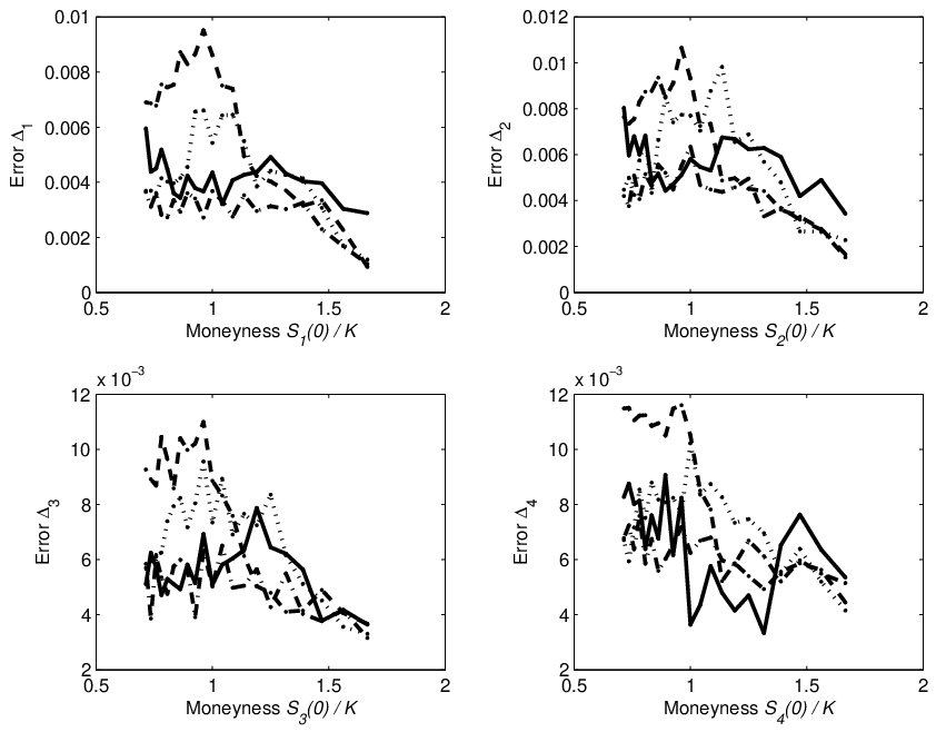
Refer to caption — Figure 1: Call Option with Fixed Strike, $M=4$ : Estimation Errors.
Adaptive: Solid Line, Loc. $\delta=0.01$ : Dashed line, Loc. $\delta=0.1$ : Dotted line, Loc. $\delta=0.05$ : Dash-dotted line.

5.2 Digital Call

The aim of this subsection is to describe the results of our numerical investigation assuming Asian digital options. The following discussion and description have a double purpose. Since the payoff of digital option can be seen as the derivative (in the sense of distribution) of the payoff of a call option, the methodology and the localization parameters described in Section 3.1 can be be rearranged and used to compute the Gamma (and cross sensitivities in the multidimensional setting) of a call option (naturally with some changes). In addition, the Delta of a digital option is a more demanding task due to the irregular payoff that is pathologically not differentiable.

We repeat the organization of our discussion as done for the Asian call options and consider only a fixed strike price. Table 4 shows the estimated multidimensional Deltas and their errors for an at-the-money digital option on $M=10$ underlying securities. The best accuracy with the standard localization technique is not achieved anymore with $\delta=1\%$ , that means that in some situations it is not the optimal choice. In contrast, the adaptive localization is the best performing technique in terms of precision. It returns better localization parameters that provide an unbiased estimator with lower variance.

Adaptive		Localization						Fin. Diff.
		$\delta=1\%$		$\delta=5\%$		$\delta=10\%$		$\delta=1\%$
$\Delta$	$\pm err$	$\Delta$	$\pm err$	$\Delta$	$\pm err$	$\Delta$	$\pm err$	$\Delta$	$\pm err$
$0.30$	$0.15$	$0.30$	$0.75$	$0.31$	$3.8$	$0.30$	$0.18$	$0.30$	$0.19$
$0.29$	$0.23$	$0.29$	$0.86$	$0.31$	$3.5$	$0.29$	$0.31$	$0.29$	$0.27$
$0.29$	$0.29$	$0.30$	$0.74$	$0.31$	$3.6$	$0.29$	$0.31$	$0.28$	$0.34$
$0.29$	$0.45$	$0.29$	$0.80$	$0.30$	$3.2$	$0.28$	$0.38$	$0.28$	$0.45$
$0.29$	$0.48$	$0.29$	$0.78$	$0.31$	$3.6$	$0.28$	$0.41$	$0.26$	$0.49$
$0.29$	$0.56$	$0.29$	$0.88$	$0.31$	$3.4$	$0.27$	$0.49$	$0.25$	$0.49$
$0.28$	$0.56$	$0.28$	$0.82$	$0.31$	$3.6$	$0.27$	$0.64$	$0.24$	$0.65$
$0.27$	$0.55$	$0.28$	$0.98$	$0.30$	$3.6$	$0.25$	$0.48$	$0.23$	$0.50$
$0.27$	$0.58$	$0.28$	$0.80$	$0.29$	$3.9$	$0.24$	$0.72$	$0.22$	$0.77$
$0.27$	$0.60$	$0.27$	$0.86$	$0.30$	$3.4$	$0.24$	$0.70$	$0.20$	$0.60$

Table 4: Digital Option with Fixed Strike,

M=10

: At-the-Money Deltas and Errors.

As done before, we run a QMC simulation considering only $M=4$ assets and analyze the results by varying the strike price. Figure 3 and 4 show the estimated Deltas and errors, respectively. Once more the adaptive localization approach displays the lowest error.

5.3 Exotic Option

As a last experiment we perform a QMC numerical simulation in order to estimate the Deltas of an exotic option. Table 5 and Figures 5 and 6 present the results of this experiment. In this last example all the approaches perform equally well, and the exotic structure of the payoff makes its estimator unsensitive to the different localization parameter. The finite difference is also performing well but is less precise if we take into account the computational burden that is $2.61$ times higher.

Adaptive		Localization						Fin. Diff.
		$\delta=1\%$		$\delta=5\%$		$\delta=10\%$		$\delta=1\%$
$\Delta$	$\pm err$	$\Delta$	$\pm err$	$\Delta$	$\pm err$	$\Delta$	$\pm err$	$\Delta$	$\pm err$
$6.4$	$1.1$	$6.5$	$1.3$	$6.5$	$1.8$	$6.5$	$0.8$	$6.5$	$1.0$
$6.6$	$1.6$	$6.6$	$1.2$	$6.6$	$1.8$	$6.6$	$1.0$	$6.6$	$1.1$
$6.8$	$1.3$	$6.7$	$1.2$	$6.7$	$1.9$	$6.7$	$0.9$	$6.8$	$1.3$
$7.0$	$1.5$	$6.9$	$1.4$	$6.9$	$1.7$	$6.9$	$1.2$	$6.9$	$2.0$
$7.2$	$1.9$	$7.0$	$1.1$	$7.0$	$1.8$	$7.1$	$1.1$	$7.1$	$2.0$
$7.4$	$1.5$	$7.2$	$1.4$	$7.2$	$1.8$	$7.2$	$1.3$	$7.3$	$2.2$
$7.6$	$1.7$	$7.3$	$1.4$	$7.3$	$1.9$	$7.4$	$1.3$	$7.5$	$2.1$
$7.8$	$1.9$	$7.5$	$1.5$	$7.5$	$1.6$	$7.5$	$1.7$	$7.7$	$2.1$
$8.0$	$2.1$	$7.6$	$1.5$	$7.6$	$1.7$	$7.7$	$1.4$	$7.9$	$2.4$
$8.2$	$1.7$	$7.8$	$1.7$	$7.8$	$1.8$	$7.9$	$1.5$	$8.1$	$1.8$

Table 5: Exotic,

M=10

: At-the-Money Deltas and Errors (

\times 100

6 Concluding Remarks

In this paper we have investigated the use of Malliavin calculus in order to calculate the Greeks of multiasset complex path-dependent options by QMC simulation. As a first result we have derived the multidimensional version of the formulas obtained by Montero and Kohatsu-Higa [11] in the single asset case.The multidimensional setting shows the advantage of the Malliavin Calculus approach over alternative techniques that have been previously proposed. These different techniques are hard to implement and in particular, are computationally time consuming when considering multiasset derivative securities. In addition, their estimators potentially display a high variance (see for instance Chen and Glasserman [1]). In contrast, the use of the generalized integral by part formula of Malliavin Calculus gives enough flexibility in order to find unbiased estimators with low variance. In the multidimensional context, we have found convenient formulas that are easy and flexible to employ and permit to improve the localization technique. Finally, we have performed a detailed analysis on how the localization parameters can influence the precision of the estimators. Moreover, we have proposed an alternate approach, based on adaptive (Q)MC techniques that returns convenient parameters that can be obtained on the flight in the simulation. This approach provides a better precision with the same computational burden. However further studies would be necessary to enhance its accuracy assuming different dynamics and payoff functions.

The proposed procedures, coupled with the enhanced version of Quasi-Monte Carlo simulations as illustrated in Sabino [16], are discussed based on the numerical estimation of the Deltas of call, digital Asian-style and Exotic basket options with a fixed and a floating strike price in a multidimensional Black-Scholes market.

References

(1) N. Chen and P. Glasserman. Malliavin Greeks without Malliavin Calculus. Stochastic Processes and their Applications, 117:1689–1723, 2007.
(2) E. Fournié, J. Lasry, J. Lebuchoux, P. Lions, , and N. Touzi. Applications of Malliavin Calculus to Monte-Carlo Methods in Finance. Finance and Stochastics, pages 391–412, 1999.
(3) M. B. Giles. Vibrato Monte Carlo Sensitivities. In Monte Carlo and Quasi-Monte Carlo Methods 2008. Springer-Verlag, 2009.
(4) P. Glasserman. Monte Carlo Methods in Financial Engineering. Springer-Verlag New York, 2004.
(5) J. Imai and K.S. Tan. A General Dimension Reduction Technique for Derivative Pricing. Journal of Computational Finance, pages 129–155, 2006.
(6) B. Jourdain. Adaptive Variance Reduction Techniques in Finance. Advanced Financial Modelling, Radon Series Comp. Appl. Math., Ed. H. Albrecher, W. Runggaldier, W. Schachermayer and de Gruyter, pages 205–222, 2009.
(7) A. Kohatsu-Higa and R. Pattersson. Variance Reduction Methods for Simulation of Densities on Wiener Space. SIAM, 40(2), 2002.
(8) P: L’Ecuyer. On the Interchange of Derivative and Expectation for Likelihood Ratio Derivative Estimators. Management Science, page 738748, 1995.
(9) J. Matoušek. On the $L^{2}$ -Discrepancy for Anchored Boxes. Journal of Complexity, 14:527–556, 1998.
(10) M. Montero and A. Kohatsu-Higa. Malliavin Calculus Applied to Finance. Physica A, 320:548–570, 2003.
(11) M. Montero and A. Kohatsu-Higa. Malliavin Calculus in Finance. Handbook of Computational and Numerical Methods in Finance, pages 111–174, 2004.
(12) H. Niederreiter. Random Number Generation and Quasi-Monte Carlo Methods. S.I.A.M. Philadelphia, 1992.
(13) D. Nualart. Malliavin Calculus and Related Topics. Springer-Verlag, Berlin, 2006.
(14) A. Owen. Latin Supercube Sampling for Very High-dimensional Simulations. ACM Transaction on Modelling and Computer Simulation, 8:71–102, 1998.
(15) A.B. Owen. Variance with Alternative Scrambling of Digital Nets. ACM Transaction of Modelling and Computer Simulation, pages 363–378, 2003.
(16) P. Sabino. Efficient Quasi-Monte Simulations for Pricing High-dimensional Path-dependent Options. Decision in Economics and Finance, 32(1):48–65, 2009.
(17) P. Sabino. Implementing Quasi-Monte Carlo Simulations with Linear Transformations. Computational Management Science, 2009. Forthcoming.
(18) S.E. Shreve. Stochastic Calculus for Finance, volume 2. Springer, 2004.
(19) I.M. Sobol’. Uniformly Distributed Sequences with an Additional Uniform Property. USSR Journal of Computational Mathematics and Mathematical Physics, 16:1332–1337, 1976. English Translation.