Photonic band-gap properties for two-component slow light
Abstract
We consider two-component ”spinor” slow light in an ensemble of atoms coherently driven by two pairs of counterpropagating control laser fields in a double tripod-type linkage scheme. We derive an equation of motion for the spinor slow light (SSL) representing an effective Dirac equation for a massive particle with the mass determined by the two-photon detuning. By changing the detuning the atomic medium acts as a photonic crystal with a controllable band gap. If the frequency of the incident probe light lies within the band gap, the light tunnels through the sample. For frequencies outside the band gap, the transmission probability oscillates with increasing length of the sample. In both cases the reflection takes place into the complementary mode of the probe field. We investigate the influence of the finite excited state lifetime on the transmission and reflection coefficients of the probe light. We discuss possible experimental implementations of the SSL using alkali atoms such as Rubidium or Sodium.
pacs
42.50.Ct, 03.65.PmI Introduction
Over the last decade there has been a great deal of interest in slow [1], stored [2, 3, 4, 5, 6, 7] and stationary [8, 9] light. Coherent control of slow light leads to a number of applications, such as generation of non-classical states in atomic ensembles and reversible quantum memories for slow light [10, 11, 12, 13, 14, 15, 16, 17], as well as non-linear optics at low intensities [18, 19, 20]. Furthermore, propagation of light through moving media [21, 22, 23, 24, 25, 26, 27, 28, 29] can be used for rotational sensing devices. Slow light is formed in an atomic medium with a -type linkage pattern (Fig. 1a) under conditions of Electromagnetically Induced Transparency (EIT) [30, 31, 32, 13, 20]. The -scheme involves two atomic ground states and an excited state, as shown in Fig. 1a. EIT emerges due to the destructive interference between atomic transitions from different ground states to a common excited state induced by a weak probe beam and a stronger control beam [30, 31, 13, 20]. EIT allows to transmit a resonant probe beam through an otherwise opaque atomic medium coherently driven by a control laser field and forms the basis of many interesting applications as e.g. creating stationary excitations of light [33, 34, 35, 36, 37] in more complex double schemes as shown in Fig. 1b, Bose-Einstein condensation of photons [36, 38], or artificial magnetic fields [39, 37] for photons.
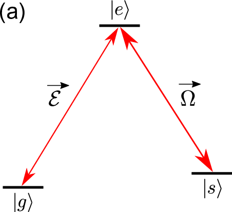
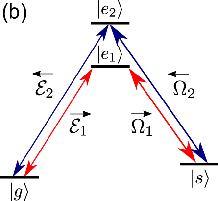
It is to be pointed out that both ordinary and double schemes support a single component slow and stationary light driving a single atomic coherence . By adding an additional control laser which couples an excited state to an additional ground state, one arrives at a tripod linkage pattern [40] characterized by two atomic coherences. However, in that case the slow light excitations remain in a single component, because the original and additional control laser beams induce transitions to a special superposition of the atomic ground states and thus effectively drive a single atomic coherence [41, 42, 43, 44].
In a recent letter [45] it has been demonstrated that two-component slow light can be produced by means of a tripod scheme which uses two standing wave control fields made of two pairs of counter-propagating laser beams, as illustrated in Fig. 2. Due to the formal similarity to two-component spinors we term the two-component slow-light ”spinor” slow light (SSL). We note however that their transformation properties under Lorentz transformations are not those of Dirac spinors. Employing two pairs of counterpropagating beams involves two atomic coherences leading to the SSL. By applying the secular approximation [33, 34], the SSL has been shown to obey an effective 1D Dirac equation [45]. This approximation is however only justified in hot atomic gases [8, 46], because it neglects all higher wave-vector components of the atomic coherence produced by the counterpropagating beams driving the same transition.

Here we study the propagation of two probe beams in an atomic ensemble coherently driven by two pairs of counterpropagating control laser fields in a double tripod-type linkage scheme shown in Fig. 3. In contrast to [45] involving a single tripod scheme, no secular approximation is needed. Thus the double tripod scheme can be used to produce SSL not only for hot atomic gases but also for cold ones and in solids. After eliminating all atomic degrees of freedom and choosing proper amplitudes and phases of the control lasers, the electric field strengths of the SSL is described by an effective Dirac equation for a particle of finite mass determined by the two photon detuning. The Dirac equation for massive particles exhibits a finite energy gap given by the particles’ rest mass energy. Thus the atomic medium acts as a photonic crystal with a controllable band gap. If the incoming probe light frequency lies within the band gap, the light tunnels through the sample, with the tunneling length being determined by the effective Compton length of the SSL. On the other hand, for frequencies of the incoming probe light outside the band gap, the transmission probability oscillates with increasing length of the sample, so the system acts as a tunable filter for certain frequencies. In both cases reflection takes place into the complementary mode of the spinor probe field and thus is accompanied by a change in frequency. Including the finite lifetime of the atomic excited states leads to a loss term in the Dirac equation. We investigate the influence of the decay on the transmission and reflection of the SSL.
II Model
II.1 Double-tripod linkage pattern


We consider the propagation of two probe beams of light in a coherently driven atomic ensemble exhibiting a double tripod level structure depicted in Fig. 3a. The atoms are described by three hyperfine ground levels , and which are coupled to the electronic excited levels and by probe (weaker) and control (stronger) fields. Two probe beams , , with central frequencies and are tuned to the atomic transitions and . Four control laser beams couple two excited states to another two ground states , the coupling strength being characterized by Rabi frequecies , where . The control fields are strong enough to be treated as external parameters. We assume four photon resonances between the probe beams and each pair of the control lasers: , where are the frequencies of the control fields. The quantities and define the one- and two-photon detuning from the one- and two-photon resonances, respectively. Furthermore and are the frequencies of the atomic transitions and . In the following the control and probe beams are supposed to be close to two-photon resonance. The simultaneous application of the probe and control beams causes EIT in which the optical transitions from the ground states interfere destructively thus preventing population of the excited states and .
The double tripod scheme can be realized with atoms like Rubidium or Sodium containing two hyperfine ground levels with and , as illustrated in Fig. 3b. These atoms have been employed in the intial light-storage experiments based on a simpler setup [3, 2]. In the present situation the states and correspond to the magnetic sublevels with and of the hyperfine ground level, whereas the state represents the hyperfine ground state with and . The two states and correspond to the electronic excited states with and characterized by . To make a double tripod setup both probe beams are to be circular polarized and all four control beams are to be circular polarized. Note that such a scheme can be implemented by adding three extra control laser beams as compared to the experiment by Liu et al [3].
II.2 Equation for the probe fields and atoms
The electric field strength of the -th probe beam is characterized by a slowly in time varying amplitude normalized to the number of photons:
| (1) |
In the following we apply a semiclassical approach in which the dynamics of the probe fields is described by classical Maxwell equations for the amplitudes and , whereas the atomic ensemble is described by Schrödinger equations for the probability amplitudes (normalized to the atomic density) , , to find an atom at a position in the internal states , and , respectively, with . It is convenient to write down the coupled light-matter equations of motion in a matrix form. To this end we define the two component spinors , and . The following equation holds for the slowly varying amplitudes of the probe fields:
| (2) |
where the r.h.s. of this equation is due to the atomic polarizability. Here is a diagonal matrix with elements , characterizes the atom-light coupling strength (assumed to be the same for both probe fields) and is the dipole moment for the transition . Neglecting effects due to atomic motion and using the rotating wave approximation, the atomic probability amplitudes obey the set of equations:
| (3) | |||||
| (4) | |||||
| (5) |
where is a matrix of Rabi frequencies , and the dagger refers to a Hermitian conjugated matrix. On the other hand, and are the following diagonal matrices
| (6) |
where and are the detunings from the one- and two-photon resonances, respectively, and is the decay rate of the -th excited electronic level. Note that the appearance of non-zero decay rates should generally be accompanied by introducing noise operators in the equations of motion [32]. Yet in the present situation one can disregard the latter noise, since we are working in the linear regime with respect to the probe field leading to a negligible population of the excited state. Assuming that the inverse matrix exists and using Eq. (5) one can relate to and obtain
| (7) |
On the other hand, Eq. (4) relates the atomic coherence to the probe field as:
| (8) |
The last equation will serve as a starting point for the adiabatic approach. It should be noted that one can also treat the case when is a singular matrix by computing, e.g., the Moore-Penrose pseudo-inverse [47]. This case however is of no interest here, since it results in an effective double- system.
III Equations for spinor slow light
III.1 Adiabatic elimination of the excited states
The zero-order adiabatic approximation is obtained by neglecting the populations of the excited states in Eq. (8), giving
| (9) |
The higher order corrections will be considered later in Sec. V when treating the effects of finite excited state lifetimes. Initially all atoms are assumed to be in the ground level . As the Rabi frequencies of the probe fields are much smaller than those of the control fields, one can neglect the depletion of the ground level , the population of the latter determining the atomic density . Using Eqs. (7) and (9) and taking one can eliminate the atomic spin coherence and express the excited-state amplitudes via the amplitudes of the probe fields:
| (10) |
Equations (2) and (10) provide a closed set of equations for the electric field amplitudes and of the SSL.
In the following the pairs of the control beams and are taken to counter-propagate along the axis: , , where are the wave numbers of the control beams characterized by the amplitudes , with . The probe fields also counter-propagate along the axis: , , with being the central wave-vector of the -th probe beam. For paraxial beams and represent the slowly varying amplitudes which depend weakly on the propagation direction . Furthermore we assume that and . We take the amplitudes of the control beams to be time-independent, neglect their position-dependence and assume the atomic density to be homogeneous throughout the sample. The slowly varying two-component amplitude obeys the following paraxial equation:
| (11) |
where
| (12) |
is a matrix with matrix elements , is a Pauli matrix and represents the inverse group velocity matrix of slow light with
| (13) |
From now on the Rabi frequencies of the control beams are considered to have the same amplitudes: and tunable phases . The latter can be made to be and by properly choosing the phases of the atomic and radiation fields. Thus one has
| (14) |
| (15) |
where
| (16) |
is the group velocity of slow light. Furthermore by taking the detunings to have the opposite signs , the matrix simplifies to
| (17) |
It should be noted that by changing relative phase one can considerably alter the time evolution of the SSL. For zero two photon detuning, i.e. , the case of corresponds to two independent tripod schemes, whereas in the limit one recovers the double- scheme, as becomes singular.
III.2 Paraxial Dirac equation
Neglecting diffraction effects and using Eqs. (15)–(17), the equation of motion (11) takes the form
| (18) |
In the regime of slow light one has . In such a case, taking , the above equation reduces to the following Dirac equation for a massive particle:
| (19) |
Assuming a monochromatic probe field , it is convenient to rewrite Eq. (18) in terms of a complex vector and the vector of Pauli matrices
| (20) |
with
| (21) |
Equation (20) has plane wave solutions , where the column obeys the eigenvalue equation . Eigenvalues of the matrix are , where
| (22) |
is the length of the complex vector . Thus the dispersion is given by . For the slow light, , one obtains
| (23) |
Equation (23) is analogous to the dispersion of a relativistic particle with an effective mass . The latter is determined by the two-photon detuning and the relative phase of the control beams . The effective speed of light is given by the velocity . At small we have quadratic dispersion characteristic to stationary light [34, 36]. As illustrated in Fig. 4, the two dispersion branches with positive and negative effective mass are separated by a gap . Thus the atomic medium acts as a photonic crystal with a controllable band gap. For the eigenfunctions become evanescent and are characterized by an imaginary wave vector . Consequently there are no propagating waves in this range, resulting in the formation of a band-gap.

IV Reflection and transmission of the probe beam

Let us analyze the transmission of a probe beam through the atomic cloud, as well as the accompanying reflection. The atomic gas is considered to be uniform along the propagation direction from the entry point of the probe beam at to its exit at . The incoming probe field contains the first component and is monochromatic with the frequency detuned from the central frequency by the amount , where is the amplitude of the incoming field. As illustrated in Fig. 5, the probe field is transmitted through the atomic cloud with the amplitude and is reflected to the second component with the amplitude , i.e. and . This leads to the following boundary conditions for the two-component probe field
The spatial development of monochromatic probe fields is described by Eq. (20) with the formal solution . Thus one can relate the two-component probe field at the entrance and exit points by
| (30) |
Combining Eqs. (IV) and (30) one finds the reflection and transmission coefficients
| (31) | |||||
| (32) |
where the general expressions for are given in Eq. (21). In what follows we are interested in the regime of slow propagation of the probe light within the atomic cloud (). In this case simplifies to and thus
| (33) |
From Eq. (IV) it becomes clear that the reflection takes place into the complementary mode of the probe field and can be accompanied by a change in frequency, as the center frequencies of the probe fields do not have to be equal.
IV.1 Oscillations of transition and reflection amplitudes


For probe light frequencies outside the band gap , the transmission and reflection amplitudes oscillate with increasing system length. Such a behavior is characteristic to light passing through resonant cavities. Thus the system acts as a frequency filter without mirrors. For zero two-photon detuning (), the transmission and reflection amplitudes (31) and (32) simplify to
| (34) |
and
| (35) |
with . Fig. 6 illustrates the oscillatory behavior of the transmission and reflection probabilities , on the sample length for zero two-photon detuning () and non-zero detuning of the incident probe field. The complete transfer of the probe field through the sample occurs at , with being an integer. The frequency difference between two such resonance maxima is inversely proportional to the sample length . For instance, if we take the group velocity of slow light and the length of the atomic cloud as in the experiments [1, 3] and choose , the period of the oscillations is around . Note that the minima of the transfer amplitude correspond to . Thus the reflection coefficient oscillates from to the maximum value . The transmission and reflection coefficients and are seen to be sensitive to the relative phase of the laser beams . In the limit the transfer probability is approaching zero () which is accompanied by a complete reflection to the second field, i.e. . This corresponds to the creation of a photonic band-gap [48, 36] in the resulting double scheme. For the reflection is zero () and there is a complete transfer of the original field through the sample (). In that case the double tripod reduces to two independent tripod schemes. Introducing a small two-photon detuning mixes the two counter-propagating probe field components, leading to a non-zero reflection () even for .
IV.2 Tunneling of slow light

In the case where the probe light frequency lies within the band-gap ), the wave-number becomes imaginary. In such a situation, Eq. (32) describes the decay of the transmission amplitude with distance. In particular, for the reflection and transmission amplitudes (31) and (32) simplify to
| (36) |
with . The dependence of the reflection and transmission probability on the product of detuning and sample length is presented in Fig. 7. The light tunnels through the sample, the tunneling length being determined by the effective Compton length
| (37) |
In fact, a relativistic particle is known to be characterized by a Compton wavelength . In the present situation the Compton length reads , where is the effective mass of the SSL. Using Eq. (36) one can see that the transmission of the incident wave is efficient as long as the length of the gas cloud is much smaller than the Compton wavelength: . For larger values of the transmission probability falls off exponentially. This behavior is related to the fact that it is impossible to localize a particle with an uncertainty smaller than the Compton wavelength [49, 50]. Since the Compton length can be tuned by changing it is possible to experimentally study the tunneling regime .
If we take the length of atomic cloud to be and the group velocity of light is [1], the Compton length becomes of the order of the length of the atomic cloud, when the detuning is equal to . This is well within the EIT transparency window which is of the order of a in the experiment [1] and absorption losses due to a finite two-photon detuning can be neglected. In contrast to ordinary absorption, the decrease in the transmission of light through the sample is now accompanied by an increase in the reflection into the complementary mode satisfying the unitarity condition .
V Influence of losses
Let us now analyze the losses due to the finite lifetime of the excited states. For this we take into account the next order of iteration in Eq. (8) and include the decay rates and in the matrix . Assuming the decay rates to be the same for both excited states () and putting to zero the one-photon detunings , the r.h.s. of the general equation of motion (11) acquires an extra term
| (38) |
In the case of slow light () and neglecting diffraction effects one has for
| (39) |
where is the effective decay rate of the probe light fields.
Eq. (39) represents a one-dimensional Dirac equation with losses which extends the previous equation (19). As a result, one needs to replace by in the corresponding reflection and transmission coefficients. For zero probe field detuning () and , the transmission and reflection coefficient take the form
| (40) | |||||
| (41) |
where we defined
| (42) |
For a large sample size these equations simplify to
| (43) | |||||
| (44) |
The transmission coefficient decays exponentially with the system length , while the reflection coefficient stays non-zero even for infinitely long samples. For sufficiently small detuning the EIT condition [20] is fulfilled . Thus one arrives at an almost perfect reflection . In the opposite case , the EIT condition is violated and the probe fields experience strong losses leading to vanishing reflectivity. This is related to the fact that for the unitarity condition is violated leading to the reduced reflectivity.
VI Conclusions
We studied two component (spinor) slow light in an ensemble of atoms coherently driven by two pairs of counter-propagating control laser fields in a double tripod-type linkage scheme. The SSL obeys an effective Dirac equation for a massive particle. By changing the two-photon detuning the atomic medium can act as a photonic crystal with a controllable band-gap. This gap is equivalent to the rest mass energy splitting in the Dirac dispersion. We investigated the dependence of tunneling and transmission rates of the incoming probe fields on its frequency. For frequencies within the band-gap the probe light tunnels through the sample with the tunneling length given by the effective Compton wave-length of the SSL. In the case of a sample length exceeding the Compton wave length of the SSL (), the formation of the band-gap leads to the perfect reflection. In the opposite limit of a short sample length () the transmission probability is close to unity, as the SSL can not be localized below the Compton wave-length. For frequencies of the probe light outside the band-gap, the reflection and transmission coefficients exhibit an oscillatory dependence on the two-photon detuning and the sample length. This can be interpreted as a mirrorless frequency filter.
We discussed the effect of finite excited state lifetimes on transmission and reflection. For sufficiently small loss rates the reflection and transmission coefficients fulfill the unitarity condition, and the reflection takes place into the complementary mode of the SSL. Increasing the loss rates leads to non-adiabatic losses and the unitarity condition no longer holds. Finally, we proposed a possible experimental realization of two-component slow light using double tripod scheme with alkali atoms like Rubidium or Sodium.
Acknowledgements.
This work has been supported by the Research Council of Lithuania (grants No. MOS-13/2011 and VP1-3.1-ŠMM-01-V-01-001), the EU project NAMEQUAM, and the DFG projects UN 280/1 and GRK 792.References
- [1] L. V. Hau, S. E. Harris, Z. Dutton, and C. H. Behroozi, Nature, 397, 594 (1999).
- [2] D. F. Phillips, A. Fleischhauer, A. Mair, R. L. Walsworth, and M. D. Lukin, Phys. Rev. Lett., 86, 783 (2001).
- [3] C. Liu, Z. Dutton, C. H. Berhoozi, and L. V. Hau, Nature, 409, 490 (2001).
- [4] N. S. Ginsberg, S. R. Garner, and L. V. Hau, Nature, 445, 623 (2007).
- [5] U. Schnorrberger, J. D. Thompson, S. Trotzky, R. Pugatch, N. Davidson, S. Kuhr, and I. Bloch, Phys. Rev. Lett., 103, 033003 (2009).
- [6] R. Zhang, S. R. Garner, and L. V. Hau, Phys. Rev. Lett., 103, 233602 (2009).
- [7] O. Firstenberg, P. London, M. Shuker, A. Ron, and N. Davidson, Nature Physics, 5, 665 (2009).
- [8] M. Bajcsy, A. S. Zibrov, and M. D. Lukin, Nature, 426, 638 (2003).
- [9] Y.-W. Lin, W.-T. Liao, T. Peters, H.-C. Chou, J.-S. Wang, H.-W. Cho, P.-C. Kuan, and I. A. Yu, Phys. Rev. Lett., 102, 213601 (2009).
- [10] M. Fleischhauer and M. D. Lukin, Phys. Rev. Lett., 84, 5094 (2000).
- [11] G. Juzeliunas and H. J. Carmichael, Phys. Rev. A, 65, 021601(R) (2002).
- [12] A. S. Zibrov, A. B. Matsko, O. Kocharovskaya, Y. V. Rostovtsev, G. R. Welch, and M. O. Scully, Phys. Rev. Lett., 88, 103601 (2002).
- [13] M. D. Lukin, Rev. Mod. Phys., 75, 457 (2003).
- [14] M. D. Eisaman, A. Andre, F. Massou, M. Fleischhauer, A. S. Zibrov, and M. D. Lukin, Nature, 438, 837 (2005).
- [15] J. Appel, E. Figueroa, D. Korystov, M. Lobino, and A. I. Lvovsky, Phys. Rev. Lett., 100, 093602 (2008).
- [16] K. Honda, D. Akamatsu, M. Arikawa, Y. Yokoi, K. Akiba, S. Nagatsuka, T. Tanimura, A. Furusawa, and M. Kozuma, Phys. Rev. Lett., 100, 093601 (2008).
- [17] K. Akiba, K. Kashiwagi, M. Arikawa, and M. Kozuma, New J. Phys., 11, 013049 (2009).
- [18] H. Schmidt and A. Imamoglu, Opt. Lett., 21, 1936 (1996).
- [19] S. E. Harris and L. V. Hau, Phys. Rev. Lett., 82, 4611 (1999).
- [20] M. Fleischhauer, A. Imamoglu, and J. Marangos, Rev. Mod. Phys., 77, 633 (2005).
- [21] U. Leonhardt and P. Piwnicki, Phys. Rev. Lett., 84, 822 (2000).
- [22] P. Öhberg, Phys. Rev. A, 66, 021603(R) (2002).
- [23] M. Fleischhauer and S. Gong, Phys. Rev. Lett., 88, 070404 (2002).
- [24] G. Juzeliūnas, M. Mašalas, and M. Fleischhauer, Phys. Rev. A, 67, 023809 (2003).
- [25] M. Artoni and I. Carusotto, Phys. Rev. A, 67, 011602(R) (2003).
- [26] F. Zimmer and M. Fleischhauer, Phys. Rev. Lett., 92, 253201 (2004).
- [27] F. Zimmer and M. Fleischhauer, Phys. Rev. A, 74, 063609 (2006).
- [28] M. Padgett, G. Whyte, J. Girkin, A. Wright, L. Allen, P. Öhberg, and S. Barnett, Opt. Lett., 31, 2205 (2006).
- [29] J. Ruseckas, G. Juzeliūnas, P. Öhberg, and S. M. Barnett, Phys. Rev. A, 76, 053822 (2007).
- [30] E. Arimondo, Prog. Opt., 35, 257 (1996).
- [31] S. E. Harris, Phys. Today, 50, 36 (1997).
- [32] M. O. Scully and M. S. Zubairy, Quantum Optics (Cambridge University Press, Cambridge, 1997).
- [33] S. A. Moiseev and B. S. Ham, Phys. Rev. A, 73, 033812 (2006).
- [34] F. E. Zimmer, A. André’, M. D. Lukin, and M. Fleischhauer, Opt. Commun., 264, 441 (2006).
- [35] F. E. Zimmer, J. Otterbach, R. G. Unanyan, B. W. Shore, and M. Fleischhauer, Phys. Rev. A, 77, 063823 (2008).
- [36] M. Fleischhauer, J. Otterbach, and R. G. Unanyan, Phys. Rev. Lett., 101, 163601 (2008).
- [37] J. Otterbach, J. Ruseckas, R. G. Unanyan, G. Juzeliūnas, and M. Fleischhauer, Phys. Rev. Lett., 104, 033903 (2010).
- [38] F. E. Zimmer, G. Nikoghosyan, and M. B. Plenio, arXiv:1103.2391v1 (2011).
- [39] K.-P. Marzlin, J. Appel, and A. I. Lvovsky, Phys. Rev. A, 77, 043813 (2008).
- [40] R. Unanyan, M. Fleischhauer, B. W. Shore, and K. Bergmann, Opt. Commun., 155, 144 (1998).
- [41] E. Paspalakis and P. L. Knight, Phys. Rev. A, 66, 015802 (2002).
- [42] A. Raczynski, M. Rzepecka, J. Zaremba, and S. Zielinska-Kaniasty, Opt. Commun., 260, 73 (2006).
- [43] A. Raczynski, J. Zaremba, and S. Zielinska-Kaniasty, Phys. Rev. A, 75, 013810 (2007).
- [44] J. Ruseckas, A. Mekys, and G. Juzeliūnas, Phys. Rev. A, 83, 023812 (2011).
- [45] R. G. Unanyan, J. Otterbach, M. Fleischhauer, J. Ruseckas, V. Kudriašov, and G. Juzeliūnas, Phys. Rev. Lett., 105, 173603 (2010).
- [46] M. Fleischhauer, M. D. Lukin, D. E. Nikonov, and M. O. Scully, Opt. Comm., 110, 351 (1994).
- [47] A. J. Laub, Matrix analysis for Scientists and Engineers (SIAM: Society for Industrial and Applied Mathematics Philadelphia, 2004).
- [48] A. André and M. D. Lukin, Phys. Rev. Lett., 89, 143602 (2002).
- [49] R. G. Unanyan, J. Otterbach, and M. Fleischhauer, Phys. Rev. A, 79, 044101 (2009).
- [50] F. M. Toyama and Y. Nogami, Phys. Rev. A, 81, 044106 (2010).