Compact smallest eigenvalue expressions in Wishart- Laguerre ensembles with or without fixed-trace
Abstract
The degree of entanglement of random pure states in bipartite quantum systems can be estimated from the distribution of the extreme Schmidt eigenvalues. For a bipartition of size , these are distributed according to a Wishart-Laguerre ensemble (WL) of random matrices of size , with a fixed-trace constraint. We first compute the distribution and moments of the smallest eigenvalue in the fixed trace orthogonal WL ensemble for arbitrary . Our method is based on a Laplace inversion of the recursive results for the corresponding orthogonal WL ensemble by Edelman. Explicit examples are given for fixed and , generalizing and simplifying earlier results. In the microscopic large- limit with fixed, the orthogonal and unitary WL distributions exhibit universality after a suitable rescaling and are therefore independent of the constraint. We prove that very recent results given in terms of hypergeometric functions of matrix argument are equivalent to more explicit expressions in terms of a Pfaffian or determinant of Bessel functions. While the latter were mostly known from the random matrix literature on the QCD Dirac operator spectrum, we also derive some new results in the orthogonal symmetry class.
1 Introduction
The theory of random matrices finds applications to the most diverse physical situations, and Wigner and Dyson are usually referred to as the pioneers of this field for their works on nuclear spectra. However, many years before their seminal papers, John Wishart had already introduced random covariance matrices in his studies on multivariate populations [1]. The Wishart ensemble (also named Laguerre or chiral, and called WL hereafter) contains random covariance matrices of the form where is a matrix with i.i.d. Gaussian entries (real, complex or quaternions labelled by the Dyson index respectively). The joint probability density function (jpdf) of its non-negative eigenvalues is given in Eq. (2.8). A related ensemble of random matrices is the fixed-trace Wishart-Laguerre (FTWL), which contains WL matrices with a prescribed trace and whose eigenvalue jpdf is given in (2.10). Recent results about the density of eigenvalues of FTWL matrices can be found in [2, 3, 4]. The study of fixed and bounded trace ensembles of non-chiral random matrices has however a longer history [5]. In [6, 7] the spectral density of the related, fixed trace Gaussian Unitary Ensemble was computed explicitly for finite , while for works on non-chiral fixed trace -ensembles we refer to [8, 9].
Two recent applications of WL and FTWL ensembles that motivate our study are effective theories of Quantum Chromodynamics (QCD) and QCD-like theories, where we refer to [10] for a most recent review and references, and the statistical theory of entangled random pure states in bipartite systems, see [11] for an excellent review, respectively.
Entanglement is indeed one of the most distinctive features of quantum systems, and it is a crucial resource in quantum computation issues, as performances of quantum computers will heavily rely on the possibility of producing states with large entanglement [12, 13]. In order to quantify the degree of entanglement of a given quantum state, it is useful to introduce an unbiased benchmark of states with the lowest degree of built-in information: pure bipartite systems (defined below) with a Hamiltonian of size constitute a typical example where well-behaved entanglement quantifiers can be defined, such as the von-Neumann or Rényi entropies of either subsystem [13], the so called concurrence for two-qubit systems [14] or other entanglement monotones [15, 16].
The main focus of this paper is on the cumulative distribution and density of the smallest FTWL eigenvalue and its relation to the corresponding quantity for the unconstrained WL ensemble: these two distributions arise naturally in the two settings described above (entanglement and QCD, respectively). The upshot is that the smallest Schmidt eigenvalue (a relevant quantity in the entanglement setting discussed below) is precisely given by the smallest eigenvalue of one of the FTWL ensembles with . Which of these ensembles to choose depends on the global symmetry of the quantum system, and we will report on the orthogonal () and unitary () symmetry classes, but not on the symplectic () class. Another application of the smallest FTWL eigenvalue is related to the Demmel condition number [17], which quantifies how hard certain numerical problems about matrix inversion are.
The results of this paper can be grouped into two parts:
- 1.
First, we study the full distribution of the smallest eigenvalue of FTWL orthogonal ensemble () at finite .
- 2.
Next, we take the large- limit of the smallest eigenvalue with fixed (the so-called microscopic limit) for both .
Let us summarize first which results were previously known for both FTWL and unconstrained WL:
- •
For FTWL ensemble at finite , the full distribution of the smallest eigenvalue was derived for and in [18]11 1 In studying the distribution of the Demmel condition number, Edelman [19] has derived the same formulae in a completely different setting. An exact mapping between the two problems is possible, but nontrivial [20, 21]., and for in [11]. In [18], a conjecture by Znidaric [22] was proven for the first moment. For general real and , where , Chen et al. [23] reported formal expressions for the smallest eigenvalue cumulative distribution and density in terms of cumbersome sums of Jack polynomials. More explicit expressions are given for the case in terms of finite sums.
- •
For WL ensemble at finite , the first results for the smallest eigenvalues of the orthogonal WL ensemble go back to Edelman [24, 25] who gave a recursive prescription. Curiously, analogous recurrence relations for have not been worked out to date, while for a closed expression exists in terms of determinants [26]. These results were extended by Forrester [27] to the case of real for special values of . Forrester again waived some limitations on and further generalized these results [28]. The most up-to-date and general formula for the smallest eigenvalue distribution involves hypergeometric function of matrix argument (HFMA), see eq. 2.13b in [28], as well as our Appendix A. Note that for this requires to be odd. For expressions in terms of Pfaffians were reported [29], with the same restriction for , and for the values of are half-integers.
The next natural step is to take the large limit for the smallest eigenvalue. For real keeping fixed, this was done in [28] for the WL and subsequently in [23] for FTWL ensembles, expressing them in terms of HFMA. It turned out that in this large limit (after a suitable rescaling) the fixed trace constraint does not matter, and in that sense the results are universal (for a different limit, namely fixed, see the recent paper [30]).
The issue of universality in the fixed (or bounded) trace ensembles had been addressed earlier in the literature, mainly for the non-chiral ensembles. It was shown in [6] that in the macroscopic large limit where the oscillations of the density are smoothed, the semi-circle or its generalizations can be matched in the constrained and unconstrained ensembles. In contrast, the higher order connected correlators become non-universal when considering non-Gaussian generalized WL ensembles, with a polynomial potential in in the exponent. On the other hand, in the microscopic limit in the bulk of the spectrum, where the oscillatory behavior of the density is zoomed into, the constraint was found to be immaterial and the universality of the sine-kernel was established in [31]. The same result was provided later in a mathematically more rigorous way for non-invariant generalizations of WL in [32, 33].
Because of this universality (i.e. constraint-independence), it is extremely useful to recall the large results derived independently for the smallest eigenvalue distributions in the application of unconstrained WL ensembles to QCD [34, 35, 36]. Here also non-Gaussian generalisations of WL were considered, and determinantal or Pfaffian expressions of Bessel functions were derived for [35] and [36], respectively. In fact much more general results were derived there, including an arbitrary number of characteristic polynomials of random matrices (so-called mass terms) in the weight function. In the second part of this paper we will show how these results in the QCD literature and the aforementioned ones in terms of HFMA are related.
The presentation of the paper is organized as follows.
In order to be self-contained in section 2 we provide some background material about the relation between bipartite entanglement and FTWL
(subsection 2.1). In subsection 2.2 we give definitions and notations used for WL and FTWL ensembles. The reader familiar to either or both of these topics
may skip the corresponding subsection(s).
In the next section 3 we derive our new results for FTWL ensembles at for arbitrary finite and , both for odd and even . There we briefly recall the results for standard WL by Edelman on which we heavily rely. This section also contains our results for arbitrary moments in subsection 3.3 and numerical checks in 3.4.
Section 4 brings us to the universal microscopic limit for fixed . It provides equivalence proofs between the known results from the QCD Dirac spectrum literature, given in subsection 4.2, and the very recent results in terms of HFMA, given in subsection 4.1. In subsection 4.3 we explicitly compute the large limit of the scaled smallest eigenvalue for and from their finite expressions and confirm the universality results. For the above mentioned equivalence is established in subsection 4.4, and for in subsection 4.5, including new results for the cumulative distribution and for even . We also report on the general scaling for moments in subsection 4.6 before concluding.
Some technical details about the definition of HFMA and a universality check for and are deferred to the appendices.
2 Bipartite entanglement and FTWL ensembles
2.1 Bipartite entanglement
Let be a -dimensional Hilbert space which is bipartite as , where without loss of generality. For example, may be taken as a given subsystem (say a set of spins) and may represent the environment (e.g., a heat bath). Let and be two complete bases of and respectively. Then, any quantum state of the composite system can be decomposed as:
| (2.1) |
where the coefficients ’s form the entries of a rectangular matrix .
In the following, we will consider entangled random pure states . This means that:
- 1.
cannot be expressed as a direct product of two states belonging to the two subsystems and .
- 2.
the expansion coefficients are random variables drawn from a certain probability distribution (see below).
- 3.
the density matrix of the composite system is simply given by with the constraint , or equivalently .
We will not consider statistically mixed states here, and we refer to [37] and references therein for recent results on mixed states.
The density matrix of a quantum state is a very important quantity as it allows to compute expectation values of observables. For an entangled pure state of a bipartite quantum system it can then be straightforwardly written as:
| (2.2) |
where the Roman indices and run from to and the Greek indices and run from to .
In some applications, it is useful to separate the contribution of the subsystem under consideration from the environment . Expectation values of observables on the system can be obtained by “tracing out” the environmental degrees of freedom (i.e., those of subsystem ) and defining the reduced density matrix as:
| (2.3) |
Using the expansion in Eq. (2.2) one gets
| (2.4) |
where ’s are the entries of the covariance matrix .
Proceeding further, one could also obtain the reduced density matrix of the subsystem in terms of the matrix and find that and share the same set of nonzero (positive) real eigenvalues , called Schmidt eigenvalues.
In the basis of eigenvectors of , one can express as
| (2.5) |
where ’s are the normalized eigenvectors of . The original composite state in this diagonal basis reads:
| (2.6) |
Eq. (2.6) is known as the Schmidt decomposition, and the normalization condition , or equivalently , imposes a constraint on the eigenvalues, .
In the Schmidt decomposition (2.6), each state is separable, but their linear combination (depending on the set of Schmidt eigenvalues) cannot, in general, be written as a direct product of two states of the respective subsystems, i.e. it is entangled. Knowledge of the Schmidt eigenvalues of the matrix is therefore essential in providing information about how entangled a pure state is.
For random pure states, the expansion coefficients in eq. (2.1) can be typically drawn from an unbiased (so called Hilbert-Schmidt) distribution
| (2.7) |
The meaning of eq. (2.7) is clear: all normalized density matrices are sampled with equal probability, which corresponds to having minimal a priori information about the quantum state under consideration. This in turn induces nontrivial correlations among the Schmidt eigenvalues (which are now real random variables between and whose sum is ) and makes the investigation of several statistical quantities about such states quite interesting. The jpdf of Schmidt eigenvalues for a Hilbert-Schmidt distribution of coefficients was derived in [38] and turns out to be exactly of the FTWL form (2.10) with , where the Dyson index corresponds respectively to real and complex matrices22 2 These two cases in turn correspond to quantum systems whose Hamiltonians preserve () or break () time-reversal symmetry.. The delta constraint there indeed guarantees a proper normalization of the reduced density matrix .
Why is the smallest Schmidt eigenvalue distribution interesting at all? We first note that due to the constraint and the fact that all eigenvalues are nonnegative, it follows that and . Now consider the following limiting situations. Suppose that the smallest eigenvalue takes its maximum allowed value . Then it follows immediately that all the remaining eigenvalues must be also identically equal to . In this situation eq. (2.6) tells us that is maximally entangled. On the other hand, if (i.e., it takes its lowest allowed value) or close to , while this will not provide much information about the degree of entanglement of , it actually tells us that one component in the Schmidt decomposition (2.6) can be safely ignored. In other words, the ’effective’ dimension of the Hilbert space has been reduced from to . The proximity of the smallest eigenvalue to zero, therefore, gives information about the efficiency of this dimensional reduction process.
For more references on entangled random pure states we refer to [11].
2.2 WL Ensembles with and without fixed trace
The jpdf of non-negative eigenvalues of the unconstrained WL ensemble is given by:
| (2.8) |
where is a known normalization constant:
| (2.9) |
and is the Vandermonde determinant.
On the other hand, the jpdf of the eigenvalues of the FTWL ensemble is given by:
| (2.10) |
For it coincides with the distribution of Schmidt eigenvalues, where the delta function guarantees that . The normalization constant for reads [20]:
| (2.11) |
The presence of a fixed-trace constraint is known to have crucial consequences on (connected) spectral correlation functions, both for finite- and in the macroscopic large- limit [6, 39]. However, in the microscopic large- limit the correlations become universal, and we shall exploit this in the next section. Let us first introduce the crucial quantities for this paper, the cumulative distributions (also called gap-probabilities), and the corresponding densities for the smallest eigenvalue of both ensembles:
| (2.12) | |||||
| (2.13) | |||||
| (2.14) | |||||
| (2.15) |
where the superscript distinguishes fixed-trace and ordinary WL. We have the following normalization conditions:
| (2.16) | |||
| (2.17) |
The th moments of the smallest Schmidt and WL eigenvalue are then given by
| (2.18) | |||||
| (2.19) |
where we define for later convenience. All density correlation functions and thus also the smallest eigenvalue distribution in ensembles with and without fixed trace can be related via an inverse Laplace transform, see e.g. [31] 33 3 For this reason we have kept the fixed trace to be a free parameter in the jpdf (2.10).. For the smallest eigenvalue distribution this relation reads:
| (2.20) | |||||
This is the main technical tool we use in the next section. For finite we are going to use known explicit expressions for WL smallest eigenvalue densities in order to derive the sought density for FTWL via the inverse Laplace transform of eq. (2.20).
3 New results for FTWL ensemble at finite and
In this section we will focus on the ensemble only. Our strategy is very simple. We will take the known results for the standard WL ensemble at any finite derived by Edelman [25] and invert the Laplace transform in eq. (2.20). The same strategy was followed by Chen et al. [23], however, they applied the inverse Laplace transform directly to the HFMA result by Forrester [28] valid for real . This led to expressions that are formally exact, but not very transparent or manageable. Furthermore, in contrast to [23, 28] we will not be restricted to odd for . The special case for was derived independently in [19] and [18].
3.1 Odd
We begin with the simpler case. Edelman [25] states that the smallest eigenvalue distribution for a WL ensemble with and odd can be written as follows:44 4 Compared to the notation in [25] we spell out the parameter explicitly contained in there.
| (3.1) |
where is a polynomial of degree and is the following constant:
| (3.2) |
As such, can be written as:
| (3.3) |
with some rational coefficients , which depend also on . The polynomial is determined via a simple recursion relation explicitly given in [25]. In addition, a simple Mathematica® code is given in Appendix A of [25] to generate the . The first two polynomials read:
| (3.4) |
and so on using the given recursion. In (3.4), is a generalized Laguerre polynomial55 5 Note a typo in Lemma 4.5. in [25] in the representation of ..
Now, it is easy to observe that (no matter what the coefficients are) the form (3.1) lends itself to a very friendly Laplace inversion. More precisely, take the inverse Laplace transform of the fundamental relation (2.20) after inserting eq. (3.3) into (3.1). One obtains:
| (3.5) | |||||
Computing the inverse Laplace transform and setting , one gets the final general formula:
| (3.6) | |||||
where is the Heaviside step function. This equation is our first main result of this section. The algorithm to compute for odd works as follows:
To give some explicit examples we have worked out in all detail the cases , which are based on eq. (3.4):
| (3.7) | |||||
| (3.8) | |||||
We stress, however, that the general formula (3.6) and the algorithm above provide an explicit and user-friendly solution to the problem of computing for any desired value of . The obtained results are much more explicit and manageable than those expressed in terms of a finite sum over partitions in [23]. To illustrate our algorithm we have generated examples with higher .
We wrote a simple Mathematica® code that generates explicit expressions for the smallest eigenvalue density (the code is freely available on demand). A plot for different values of odd and is provided in fig. 1.

3.2 Even
Now, we turn to the more complicated case even. Also in this case, we can derive a general formula for involving the same polynomial coefficients as in Edelman’s recursion. To the best of our knowledge, apart from [18], no such expressions were previously known for the FTWL ensemble.
Edelman [25] states that the smallest eigenvalue distribution for a WL ensemble with and even can be written as follows:
| (3.9) |
where and are polynomials of degree at most , and is given in eq. (3.2). The two related functions and are defined as follows:
| (3.10) |
where is a Tricomi confluent hypergeometric function given by:
| (3.11) |
Let us now write the polynomials and as:
| (3.12) | |||||
| (3.13) |
with some rational coefficients and , which depend also on . As in the odd case they follow from a recurrence relation given in [25] along with a Mathematica® code to generate them. The first two examples read:
| (3.14) | |||||
| (3.15) |
Applying now eq. (2.20) to (3.9), we get:
| (3.16) |
where
Here we have inserted the integral representation (3.11).
Taking the inverse Laplace transform of the quantities in square brackets, and setting we can eventually write:
| (3.17) |
where:
| (3.18) | |||||
| (3.19) | |||||
In the second step we have performed the integrals and applied some simple algebra, and is a standard hypergeometric function.
Eq. (3.17) together with eqs. (3.18) and (3.19) is the second result of this section. Again, the algorithm to compute for even works as follows:
To provide explicit examples we give the expressions for based on eqs. (3.14) and (3.15), where the result for was previously derived in [18]:
| (3.20) | |||||
and
| (3.21) |
where:
| (3.22) | |||||
| (3.23) | |||||
In order to illustrate our algorithm above we again wrote a simple Mathematica® code that generates explicit expressions for the smallest eigenvalue density. A plot for different even and as an example is provided in fig. 2.
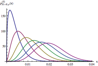
3.3 Moments for odd
Arbitrary moments can be computed easily in a closed form for odd from eq. (3.6), using the following integral formula:
| (3.24) |
Here is Euler’s Beta function. We thus obtain
| (3.25) | |||||
To give an example, the th moment for is given as follows:
In particular for the first moment or average value we get the following answer
| (3.26) |
For comparison at the large- behavior is as follows [18]:
| (3.27) |
where:
| (3.28) |
(compare with subsection 4.6). Although the computation of moments for even is possible, based on our explicit expressions given previously, we did not find short closed expressions as in eq. (3.25) above.
3.4 Numerical checks
In fig. 3 we compare a few theoretical densities from the previous subsections 3.1 and 3.2 for finite with the corresponding numerical results. These are obtained as follows [20, 21]:
- 1.
we generate real Gaussian matrices (where ).
- 2.
for each instance we construct the Wishart matrix .
- 3.
we diagonalize and collect its real and non-negative eigenvalues .
- 4.
we define a new variable as .
- 5.
we construct a normalized histogram of .
The agreement between theory and simulations is excellent.

4 Equivalence proofs and new results in the large- limit
We now turn to the microscopic large- limit for the orthogonal and unitary ensembles (), with fixed. More precisely, let us define the following microscopic scaling limits at the origin:
| (4.1) | |||||
| (4.2) |
Notice that the mean level spacing at the origin (the -dependent rescaling factor) is different for FTWL and standard WL ensembles. This fact was also observed when comparing the corresponding macroscopic densities in the Gaussian ensembles with and without constraint [6].
It has been shown that in the microscopic limit (i) the smallest eigenvalue distribution in non-Gaussian generalizations of WL ensembles is universal [35, 36], and (ii) for all real , the microscopic limit for the smallest eigenvalue distribution is the same for WL and FTWL ensembles in all cases where a representation in terms of HFMA exists [23]. We also recall that universality (ii), that is the independence of the constraint, was shown earlier for all microscopic density correlation functions in the bulk of the spectrum for unitary non-chiral ensembles for monic even potentials [31] or i.i.d. matrix elements [32, 33].
Building on [23], from now on we shall assume that:
| (4.3) | |||||
| (4.4) |
for all and . Therefore, there is no reason to keep the superscripts (WL) and (FT). We will thus use the unified notation and , labeled by only66 6 We note in passing that the large behavior of is known from [40], see also [42] for the calculation of leading term using a Coulomb gas method.. Note that one still has
| (4.5) | |||
| (4.6) | |||
| (4.7) |
What are the known results for and ? It turns out that two communities have derived different formulae for these very same quantities using different languages: HFMA on the one side, and determinants or Pfaffians of Bessel functions on the other side (see two next subsections). It is one of the goals of this paper to highlight this connection, which is not widely appreciated, and to actually prove the equivalence of these formulae by simple algebraic methods. As a result of this (and of the previous section) we will derive some new compact results in the second language in cases where only HFMA or no results were previously known.
We should also mention here that a third way exists to compute the cumulative distribution. Formally it is given by the Fredholm determinant of the corresponding Bessel kernel. This has been mapped to expressions containing a transcendent of the solution of the Painlevé V for [40] and [41]. In particular, the distributions for different s can be related to each other. However, this relation does not allow us to generate more explicit expressions in terms of determinants and Pfaffians below.
4.1 Hypergeometric functions of matrix argument (HFMA)
In order to establish the claimed equivalence we first need to state the results in the first language. Forrester [28] and Chen et al. [23] independently gave expressions for and valid for all and integer , in terms of HFMA as:
| (4.8) | |||||
| (4.9) |
where the constant is given by77 7 Note that the expression for the constant , eq. (2.15c) in [28] (and subsequently in [23]), as well as eq. (4.11) as it appears in [23] contain misprints.:
| (4.10) |
and is the identity matrix . For definitions and properties of HFMA we refer to Appendix A. We note that for integer implies that must be odd.
The formulas above were specialized in [23] to the two cases (a) for all , and (b) for , yielding respectively:
| (4.11) | |||||
| (4.12) |
where is a modified Bessel function of the first kind. The appearance of Bessel functions for special instances of formulas (4.8) and (4.9) is not at all accidental, as we will see now.
4.2 Determinants and Pfaffians of Bessel functions.
In the context of Random Matrix Theory applied to effective theories of Quantum Chromodynamics (QCD) or QCD-like theories, the large- distribution of the smallest Dirac operator eigenvalue has been studied intensely for the symmetry classes (and 4), see [10] for references. It turns out that the Dirac eigenvalues (occurring in pairs due to chiral symmetry) are precisely distributed according to the WL jpdf (2.8) upon the mapping . The relation between the smallest Dirac eigenvalue , and the smallest WL eigenvalue distribution trivially follows:
| (4.13) | |||||
| (4.14) |
where we also give the relation to the cumulative distribution in the Dirac picture. We still have and the standard normalization is ensured.
The following results hold for our symmetry classes:
| (4.15) | |||||
| (4.16) | |||||
| (4.17) | |||||
| (4.18) |
where stands for the Pfaffian of the antisymmetric matrix .
Most of these results were known in the literature, apart from the normalization constant given in eq. (4.41), and the new eq. (4.18) to be derived below. For the distribution eq. (4.15) was derived in [26, 34, 35]. For and eq. (4.17) was shown in [27], and then extended to all odd in [36] up to normalization.
We note in passing that for the distribution for is known explicitly from [27] (see eq. (4.11) and take its derivative), but the results quoted in [29] for only hold for even, that is for half-integer values of . Finally we mention that for small all distributions for can be very well approximated by using finite results [43], like in the Wigner surmise.
Turning to the corresponding cumulative distributions the following results hold:
| (4.19) |
for [35], and for and odd our new result reads
| (4.20) |
Before providing a general algebraic proof of the equivalence of the two languages in subsections 4.4 and 4.5, we can quickly check the agreement between the two different formulations above, starting from the special HFMA cases in eqs. (4.11) and (4.12). Using the map (4.14), eq. (4.19) obviously contains eq. (4.12) as a special case. Specifying in eq. (4.11) leads to the special cases () and () in eqs. (4.19) and (4.20) respectively.
4.3 Results for the scaled smallest eigenvalue distribution for and .
In this subsection, we give two results for the scaled smallest eigenvalue distribution at even and . In principle the universality eq. (4.4), that is the agreement between the WL and FTWL distributions in the microscopic large- limit, has not been shown for with even , although there is little doubt that it extends from the odd case. We explicitly check here that this is indeed the case by taking the microscopic large- limit for FTWL at starting from the known eq. (3.20) for finite- and getting to the same result as in WL. For we derive a new result that was unknown even for the microscopic limit of the unconstrained WL ensemble.
For we first recall how the known microscopic result for WL is obtained. Starting from the finite- expression eq. (3.9) together with eq. (3.14) we need to know the asymptotic limit of the Tricomi confluent hypergeometric function, in the scaling limit eq. (4.2). It was derived in Corollary 3.1 of [24], alternatively it follows from eq. 13.3.3 [44]:
| (4.21) |
Collecting all prefactors we thus obtain
| (4.22) |
The relation eq. (4.13) maps this to the eq. (4.17). This result has to be compared with the limit eq. (4.1) of eq. (3.20) in FTWL ensemble. Because the limit of the hypergeometric function is more involved we defer the derivation to Appendix B, finding complete agreement as in eq. (4.4):
| (4.23) |
This extends the expected universality to the case of even .
For the corresponding microscopic limit of (3.21) for FTWL is already rather cumbersome, involving the asymptotic of a sum of hypergeometric functions. We therefore restrict ourselves to compute the corresponding microscopic limit in the WL ensemble - which is also new - and conjecture that the universal relation eq. (4.23) extends to and in fact to all higher even ’s. Combining eqs. (3.9) and (3.15) we have to compute
Eq. (4.21) together with the Laguerre asymptotic for negative argument,
| (4.24) |
yields the following final answer,
| (4.25) |
4.4 Equivalence proofs for
In this subsection and in the following, we provide an algebraic link between the HFMA and the Bessel determinant languages in the spirit of earlier works [41, 45]. We start from the formula in eq. (4.9) which expresses the scaled smallest eigenvalue distribution (with or without fixed trace constraint) in terms of HFMA:
| (4.26) |
Next, we use the following integral representation due to Forrester [28] valid for integer values of and :
| (4.27) | |||||
where we have defined
| (4.28) |
and the Vandermonde determinant of the angles
| (4.29) |
Comparison between (4.27) and (4.26) yields and . Denoting by ⋆ complex conjugation, we can use the Andréief identity [46]
| (4.30) |
We thus obtain for the -fold integral in the second line of eq. (4.27)
| (4.31) |
where we have used the following integral representation for the modified Bessel function (valid for integer index only):
| (4.32) |
Setting in (4.31) and simplifying all prefactors, we eventually get from (4.26):
| (4.33) |
This is identical to eq. (4.15) after switching to the Dirac picture eq. (4.13).
The proof for the cumulative distribution goes along the same lines, merely changing the coefficient in front and the index shift of the Bessel function. We obtain the following from eq. (4.8) by identifying and in the representation eq. (4.27) and collecting all prefactors:
| (4.34) |
This corresponds to eq. (4.19) using the map eq. (4.14). Note that it is highly non-trivial to derive eq. (4.34) from eq. (4.33) using eq. (4.5).
4.5 Equivalence proof and new results for
We start again from the formula in eq. (4.9) expressing the scaled smallest eigenvalue distribution (with or without fixed trace constraint) in terms of HFMA:
| (4.35) |
Next, we use again the integral representation in eq. (4.27) and to write:
| (4.36) | |||||
Comparison between (4.27) and (4.35) indeed yields and . Next, we use section 11.5 in [5], combining eqs. (11.5.2) and (11.5.4) there to write
| (4.37) |
where the determinant on the right hand side is of size and indices run as follows, and .
Now we can define the two sets of functions and and thus use the de Bruijn identity [47]:
| (4.38) |
to evaluate the -fold integral in the second line of eq. (4.36):
| (4.39) |
where the indices all run from , and we have used again the integral representation for the Bessel function (4.32).
Setting in (4.39) and simplifying all prefactors, we eventually get for eq. (4.35):
| (4.40) |
where is the normalization constant:
| (4.41) |
Applying now eq (4.13), we get the distribution in the Dirac picture (4.16) including its explicit normalization constant for any , which was previously unavailable.
The proof for the cumulative distribution easily follows from (4.8), and we only quote the result which is new, after having identified and in eq. (4.36) instead:
| (4.42) | |||||
The range of indices is the same as in eq. (4.39). Once again, deriving eq. (4.42) directly from eq. (4.40)
using eq. (4.5) is highly non-trivial.
4.6 Moments for large
We point out a universal expression for the large decay of the th moment of the smallest eigenvalue, valid for both and 2:
| (4.43) |
where we have defined the universal coefficient
| (4.44) |
The scaling with different powers of trivially follows from the different spacings in the definition of the microscopic limit eqs. (4.1) and (4.2), as we will show now. Starting from the definition of the average of the smallest eigenvalue for FTWL (2.18) we have
| (4.45) |
after making a change of variable . This implies, using the limit (4.1):
| (4.46) |
The same argument for WL with a different change of variables, , leads to
| (4.47) |
Alternatively the universal right hand side can be expressed in the Dirac picture, using the map eq. (4.13), as it is given in eq. (4.44).


Let us give a few examples, by simply inserting eqs. (4.17) and (4.15) into the integral
| (4.48) | |||||
| (4.49) |
Specializing these results to the case of the first moment (average value), we obtain:
| (4.50) | |||||
| (4.51) |
in complete agreement with [11, 18] (after switching to their conventions). However, the general asymptotic relation (4.43) provided here allows to derive analogous, new results for any for which the smallest eigenvalue in the Dirac picture is known.
5 Conclusions
In this paper we addressed the smallest eigenvalue distribution in fixed-trace Wishart-Laguerre (FTWL) ensembles of random matrices, as well as its cumulative distribution and moments, and the corresponding quantity for unconstrained Wishart-Laguerre (WL) ensembles. Our motivation comes from the statistical description of entangled random pure states in bipartite systems of size , where the distribution of the smallest Schmidt eigenvalue provides useful information about the degree of entanglement of these states, and as such it has been subject to intense scrutiny in recent years.
In the first part, we derived new results for the FTWL ensemble with orthogonal symmetry. Here the constraint plays an important role, and we computed explicit expressions for the smallest eigenvalue by Laplace inverting a recursion relation given by Edelman for the unconstrained WL ensemble. In particular our results extend very recent expressions to even values of . Examples were given for several even and odd values of and checked via numerical simulations.
In the second part, we studied the microscopic large- limit at fixed , both for orthogonal and unitary ensembles. Here the constraint (after a proper rescaling) is immaterial due to universality. We proved the equivalence of two different sets of results in the literature, given in terms of either hypergeometric functions of matrix argument (HFMA), or in terms of Pfaffians and determinants of Bessel functions. Our technical tool was to translate HFMA into their multiple integral representations and to use the classical Andréief-de Brujin identities. Apart from this equivalence proof, our new results include the cumulative distributions, the universality of the smallest eigenvalue for and an explicit expression for , all in the orthogonal symmetry class. In addition we have determined the precise asymptotic behavior of all moments for large , in both symmetry classes.
Several open problems persist, in particular how to find a closed universal formula for all even values of in the orthogonal symmetry class in the microscopic limit. Furthermore, it would be interesting to extend these results to the symplectic symmetry class. Here a compact expression is only known for the special integer . The problem is the apparent lack of a suitable integral representation for HFMA in order to proceed.
Acknowledgments. We would like to thank Satya Majumdar for discussions.
Appendix A Hypergeometric functions of matrix argument (HFMA)
The hypergeometric function of a matrix argument takes a complex symmetric matrix as input and provides a real number as output. More precisely, let and be integers, and be the real eigenvalues of . We have:
| (1.1) |
where is a parameter, the symbol means that is a partition of (i.e. are integers such that ), and the following symbol is a generalized Pochhammer symbol. In (1.1), is a Jack polynomial, i.e. a symmetric, homogeneous polynomial of degree in the eigenvalues of [48, 49]. Jack polynomials generalize the Schur function, the zonal polynomial and the quaternion zonal polynomial to which they reduce for respectively. The HFMA (1.1) generalizes the ordinary hypergeometric function to which it reduces when .
The series (1.1) converges for any if ; it converges if and ; and diverges if , unless it terminates. An efficient evaluation of HFMA is now made possible by an algorithm devised by Koev and Edelman [50], which we used extensively to check numerically all the results given in terms of HFMA in this paper.
Appendix B Microscopic limit of for
In this appendix we take the microscopic limit eq. (4.1) of the smallest eigenvalue for and in FTWL eq. (3.20):
| (2.1) |
While the first factor in the second line yields an exponential prefactor,
| (2.2) |
the asymptotic limit of the hypergeometric function requires more care. Using eq. 9.132.1 in [51] we have that
| (2.3) | |||||
with
| (2.4) |
In order to apply the standard asymptotic limits, eqs. 9.121.9-10 in [51],
| (2.5) | |||||
| (2.6) |
where we identify and , we still have to shift the third index of the two hypergeometric functions in eq. (2.3). Using eq. 9.137.1 in [51] we obtain for the first
| (2.7) | |||||
and for the second
| (2.8) | |||||
Collecting all the results from above and all factors we obtain as a final result
| (2.9) | |||||
which agrees with eq. (4.22) as we have claimed.
References
- [1] J. Wishart, The generalised product moment distribution in samples from a normal multivariate population, Biometrika 20A, 32 (1928); Erratum Note on the Paper by Dr. J. Wishart in the Present Volume (XXa), ibid. 20A, 424 (1928).
- [2] H.-J. Sommers and K. Życzkowski, Statistical properties of random density matrices, J. Phys. A: Math. Theor. 37, 8457 (2004).
- [3] H. Kubotani, S. Adachi, and M. Toda, Exact formula of the distribution of Schmidt eigenvalues for dynamical formation of entanglement in quantum chaos, Phys. Rev. Lett. 100, 240501 (2008); S. Adachi, M. Toda, and H. Kubotani, Random matrix theory of singular values of rectangular complex matrices I: Exact formula of one-body distribution function in fixed-trace ensemble, Ann. Phys. 324, 2278 (2009).
- [4] P. Vivo, Entangled random pure states with orthogonal symmetry: exact results, J. Phys. A: Math. Theor. 43, 405206 (2010).
- [5] M. L. Mehta, Random Matrices (Academic Press, Third Edition, London 2004).
- [6] G. Akemann, G. M. Cicuta, L. Molinari, and G. Vernizzi, Compact support probability distributions in random matrix theory Phys. Rev. E 59, 1489 (1999); Non-universality of compact support probability distributions in random matrix theory, Phys. Rev. E 60, 5287 (1999).
- [7] R. Delannay and G. Le Caër, Exact densities of states of fixed trace ensembles of random matrices, J. Phys. A: Math. Gen. 33, 2611 (2000).
- [8] G. Le Caër and R. Delannay, The fixed-trace -Hermite ensemble of random matrices and the low temperature distribution of the determinant of a -Hermite matrix, J. Phys. A: Math. Gen. 40, 1561 (2007).
- [9] D.-S. Zhou, D.-Z. Liu, and T. Qian, Fixed trace -Hermite ensembles: Asymptotic eigenvalue density and the edge of the density, J. Math. Phys. 51, 033301 (2010).
- [10] J. J. M. Verbaarschot, Applications of Random Matrix Theory to QCD, invited chapter in “Handbook on Random Matrix Theory”, Eds. G. Akemann, J. Baik, P. Di Francesco, Oxford University Press 2011, Preprint [arXiv:0910.4134] (2009).
- [11] S. N. Majumdar, Extreme eigenvalues of Wishart matrices: application to entangled bipartite system, invited chapter in “Handbook on Random Matrix Theory”, Eds. G. Akemann, J. Baik, P. Di Francesco, Oxford University Press 2011, Preprint [arXiv:1005.4515] (2010).
- [12] M. A. Nielsen and I. L. Chuang, Quantum Computation and Quantum Information (Cambridge University Press, Cambridge, 2000).
- [13] A. Peres, Quantum Theory: Concepts and Methods, (Kluwer Academic Publishers, Dordrecht, 1993).
- [14] S. Hill and W. K. Wootters, Entanglement of a pair of quantum bits, Phys. Rev. Lett. 78, 5022 (1997); W. K. Wootters, Entanglement of formation of an arbitrary state of two qubits, Phys. Rev. Lett. 80, 2245 (1998).
- [15] V. Cappellini, H.-J. Sommers, and K. Życzkowski, Distribution of concurrence of random pure states, Phys. Rev. A 74, 062322 (2006).
- [16] G. Gour, Family of concurrence monotones and its applications, Phys. Rev. A 71, 012318 (2005).
- [17] J. W. Demmel, The probability that a numerical analysis problem is difficult, Math. Comput. 50, 449 (1988); Lu Wei, M. R. McKay, and O. Tirkkonen, Exact Demmel condition number distribution of complex Wishart matrices via the Mellin transform, IEEE Communication Letters 15, 175 (2011).
- [18] S. N. Majumdar, O. Bohigas, and A. Lakshminarayan, Exact minimum eigenvalue distribution of an entangled random pure state, J. Stat. Phys. 131, 33 (2008).
- [19] A. Edelman, On the distribution of a scaled condition number, Math. Comput. 58, 185 (1992).
- [20] K. Życzkowski and H.-J. Sommers, Induced measures in the space of mixed quantum states, J. Phys. A: Math. Gen. 34, 7111 (2001).
- [21] I. Bengtsson and K. Życzkowski, Geometry of Quantum States (Cambridge Univ. Press, New York, 2006).
- [22] M. Znidaric, Entanglement of random vectors, J. Phys. A: Math. Theor. 40, F105 (2007).
- [23] Y. Chen, D.-Z. Liu, and D.-S. Zhou, Smallest eigenvalue distribution of the fixed-trace Laguerre -ensemble, J. Phys. A: Math. Theor. 43, 315303 (2010).
- [24] A. Edelman, Eigenvalues and condition numbers of random matrices, SIAM J. Matrix Anal. Appl. 9, 543 (1988).
- [25] A. Edelman, The distribution and moments of the smallest eigenvalue of a random matrix of Wishart type, Lin. Alg. Appl. 159, 55 (1991).
- [26] P. J. Forrester and T. D. Hughes, Complex Wishart matrices and conductance in mesoscopic systems: exact results, J. Math. Phys. 35, 6736 (1994).
- [27] P. J. Forrester, The spectrum edge of random matrix ensembles, Nucl. Phys. B 402, 709 (1993).
- [28] P. J. Forrester, Exact results and universal asymptotics in the Laguerre random matrix ensemble, J. Math. Phys. 35, 2539 (1994).
- [29] T. Nagao and P. J. Forrester, The smallest eigenvalue distribution at the spectrum edge of random matrices, Nucl. Phys. B 509, 561 (1998).
- [30] E. Katzav and I. Pérez-Castillo, Large deviations of the smallest eigenvalue of the Wishart-Laguerre ensemble, Phys. Rev. E 82, 040104(R) (2010).
- [31] G. Akemann and G. Vernizzi, Macroscopic and microscopic (non-)universality of compact support random matrix theory, Nucl. Phys. B 583, 739 (2000).
- [32] F. Götze and M. Gordin, Limit correlation functions for fixed trace random matrix ensembles, Comm. Math. Phys. 281, 203 (2008).
- [33] D.-Z. Liu and D.-S. Zhou, Universality at zero and the spectrum edge for fixed trace gaussian ensembles of random matrices, J. Stat. Phys. 140, 268 (2010).
- [34] T. Wilke, T. Guhr, and T. Wettig, The microscopic spectrum of the QCD Dirac operator with finite quark masses, Phys. Rev. D 57, 6486 (1998).
- [35] S. M. Nishigaki, P. H. Damgaard, and T. Wettig, Smallest Dirac eigenvalue distribution from random matrix theory, Phys. Rev. D 58, 087704 (1998).
- [36] P. H. Damgaard and S. M. Nishigaki, Distribution of the th smallest Dirac operator eigenvalue, Phys. Rev. D 63, 045012 (2001).
- [37] V. Al. Osipov, H.-J. Sommers, and K. Życzkowski, Random Bures mixed states and the distribution of their purity, J. Phys. A: Math. Theor. 43, 055302 (2010).
- [38] S. Lloyd and H. Pagels, Complexity as thermodynamic depth, Ann. Phys. 188, 186 (1988); E. Lubkin, Entropy of an -system from its correlation with a -reservoir, J. Math. Phys. 19, 1028 (1978).
- [39] A. Lakshminarayan, S. Tomsovic, O. Bohigas, and S. N. Majumdar, Extreme statistics of complex random and quantum chaotic states, Phys. Rev. Lett. 100, 044103 (2008).
- [40] C. A. Tracy and H. Widom, Level spacing distributions and the Bessel kernel, Comm. Math. Phys. 161, 289 (1994).
- [41] P. J. Forrester, Painlevé transcendent evaluation of the scaled distribution of the smallest eigenvalue in the Laguerre orthogonal and symplectic ensembles, Preprint [nlin/0005064] (2000).
- [42] Y. Chen and S. M. Manning, Asymptotic level spacing of the Laguerre ensemble: a Coulomb fluid approach, J. Phys. A: Math. Gen. 27, 3615 (1994).
- [43] G. Akemann, E. Bittner, M. J. Phillips, and L. Shifrin, A Wigner surmise for hermitian and non-hermitian chiral random matrices, Phys. Rev. E 80, 065201 (2009).
- [44] M. Abramowitz and I. E. Stegun, Handbook of Mathematical Functions (Dover Publications Inc., New York, 1965).
- [45] R. D. Gupta and D. St. P. Richards, Hypergeometric functions of scalar matrix argument are expressible in terms of classical hypergeometric functions, SIAM J. Math. Anal. 16, 852 (1985).
- [46] C. Andréief, Note sur une relation entre les intégrales définies des produits des fonctions, Mém. de la Soc. Sci. de Bordeaux 2, 1 (1883).
- [47] N. G. de Bruijn, On some multiple integrals involving determinants, J. Indian Math. Soc. 19, 133 (1955).
- [48] R. J. Muirhead, Aspects of multivariate statistical theory (John Wiley & Sons Inc., New York, 1982).
- [49] R. Stanley, Some combinatorial properties of Jack symmetric functions, Adv. Math. 77, 76 (1989).
- [50] P. Koev and A. Edelman, The efficient evaluation of the hypergeometric function of a matrix argument, Math. Comp. 75, 833 (2006).
- [51] I. S. Gradshteyn and I. M. Ryzhik, Table of Integrals, Series, and Products (Academic Press, San Diego, 2000).