Exploring the singlet scalar dark matter from direct detections and neutrino signals via its annihilation in the Sun

In the SSDM-SM, the Lagrangian reads

where $H$ is the SM Higgs doublet. The linear and cubic terms of the scalar $S$ are forbidden by the $Z_{2}$ symmetry $S\rightarrow-S$. Then $S$ has a vanishing vacuum expectation value (VEV) $\langle S\rangle=0$ which ensures the DM candidate $S$ stable. $\lambda_{S}$ describes the DM self-interaction strength which is independent of the DM annihilation. After the spontaneous symmetry breaking (SSB), one can obtain the DM mass $m_{D}^{2}=m_{0}^{2}+\lambda\;v_{\rm EW}^{2}$ with $v_{\rm EW}=246$ GeV. The SSDM-SM is very simple and has only three free parameters: the DM mass $m_{D}$, the Higgs mass $m_{h}$ and the coupling $\lambda$. In terms of the observed DM abundance $\Omega_{\rm DM}h^{2}=0.1123\pm 0.0035$ [3], one can calculate the coupling $\lambda$ for the given $m_{D}$ and $m_{h}$. Here we take $m_{h}=125$ GeV [20] and $1\;{\rm GeV}\leq m_{D}\leq 200$ GeV for illustration. As shown in Fig. 1, the observed DM abundance requires $\lambda\sim{\cal O}(10^{-4}-1)$. It is well known that the annihilation cross section $\sigma$ will become larger for the same coupling when the annihilation process nears a resonance. This feature implies that there is a very small coupling when $0.8\;m_{h}\lesssim 2m_{D}<m_{h}$ as shown in Fig. 1. This region is named as the resonance region in the following parts of this paper.

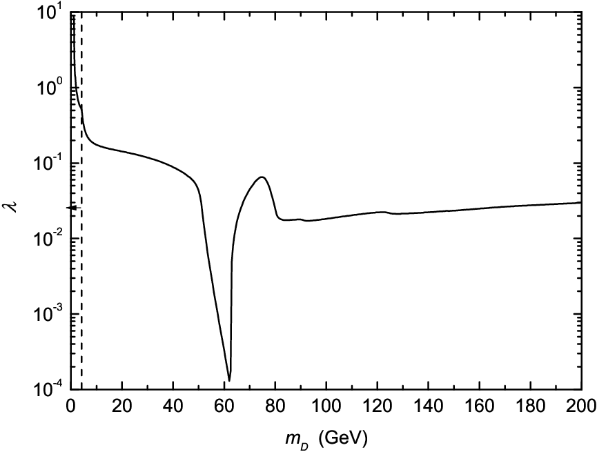
Using the predicted $\lambda$ from the observed DM abundance, one can calculate the spin-independent DM-nucleon elastic scattering cross section [21]

where $m_{n}$ is the nucleon mass and $f=(7/9)\sum_{q=u,d,s}f_{Tq}^{p}+2/9$. In terms of the relevant formulas in Ref. [8], one can calculate the parameters $f_{Tq}^{p}$ and obtain $f\approx 0.56\pm 0.17$. On the other hand, the lattice results imply $f\approx 0.29\pm 0.03$ where we take the strange-quark sigma term $16\;{\rm MeV}\leq\sigma_{s}\leq 69$ MeV [22]. Therefore we adopt $0.26\leq f\leq 0.73$ for the following analyses. The authors in Ref. [15] have discussed that the light DM particle $S$ can explain the DAMA [23] and CoGeNT [24] experiments. Here we consider the latest experiment limits and recalculate the spin-independent DM-nucleon elastic scattering cross section $\sigma_{n}^{\rm SI}$ with $0.26\leq f\leq 0.73$. Notice that $\sigma_{n}^{\rm SI}$ is not sensitive to the Higgs mass in the low DM mass range. As shown in Fig. 2 (top left panel), the predicted $\sigma_{n}^{\rm SI}$ in the region $6\;{\rm GeV}\lesssim m_{D}\lesssim 8$ GeV and $f\gtrsim 0.60$ well fit the common region of the DAMA and CoGeNT [25]. However, the recent CDMS II [26] disfavors the CoGeNT+DAMA region. We find that the CDMS II [26], CDMS (shallow-site data) [27], CRESST [28] and TEXONO [29] can exclude the $f\gtrsim 0.63$ region for $1\;{\rm GeV}\leq m_{D}\leq 10$ GeV. The $f=0.63$ case has been shown as the blue solid line in the top left panel of Fig. 2. The latest XENON100 [30] may exclude $7\;{\rm GeV}\lesssim m_{D}\lesssim 52$ GeV and a narrow region $65\;{\rm GeV}\lesssim m_{D}\lesssim 80$ GeV even if we take $f=0.26$ as shown in Fig. 2. The future experiments CDMS 100 kg [31] and XENON1T [32] can cover most parts of the allowed parameter space. As the DM mass increases, new DM annihilation channels will be open which means that the predicted $\lambda$ from the DM relic density will quickly decrease. Therefore a kink around the bottom quark mass $m_{D}\approx m_{b}=4.2$ GeV occurs in the top left panel of Fig. 2. When the DM mass approaches the resonant point $m_{D}$ = 62.5 GeV for $m_{h}$ =125 GeV, one can obtain a very large thermally averaged annihilation cross section $\langle\sigma v\rangle$ for the given $\lambda$. In order to derive the correct DM relic density, we have to require that the coupling $\lambda$ is very small. In this case, a very small $\sigma_{n}^{\rm SI}$ around the resonant point can be obtained.

The SSDM-SM also suffers other constraints except for the direct detections, such as the potential’s global minimum at $\langle h\rangle=v_{\rm EW}$ and $\langle S\rangle=0$ requires $|\lambda|<\sqrt{\lambda_{S}/2}m_{h}/v_{\rm EW}+m_{D}^{2}/v_{\rm EW}^{2}$ [13]. Since the perturbativity implies $6\lambda_{S}<4\pi$, one can derive $|\lambda|<\sqrt{\pi/3}m_{h}/v_{\rm EW}+m_{D}^{2}/v_{\rm EW}^{2}$. Then we find the desired DM relic density can exclude $m_{D}\lesssim 4.1$ GeV for $m_{h}=125$ GeV. The vertical dashed line with arrowhead in the left panels of Figs. 1 and 2 shows the excluded region. In Ref. [14], the authors have given the lower bounds on $m_{D}$ for several typical $\lambda_{S}$ based on the one-loop vacuum stability and the observed DM relic density.

We begin with a brief review of the 2HBDM described in Ref. [17]. The model is based on the gauge group $SU(2)_{L}\otimes SU(2)_{R}\otimes U(1)_{B-L}$. The left- and right-handed fermions belong to $SU(2)_{L}$ and $SU(2)_{R}$ doublets, respectively. The Higgs sector contains two Higgs bidoublets $\phi$ (2,$2^{*}$,0), $\chi$ (2,$2^{*}$,0) and a left(right)-handed Higgs triplet $\Delta_{L(R)}$ (3(1),1(3),2) with the following flavor contents

The introduction of Higgs bidoublets $\phi$ and $\chi$ can account for the electroweak symmetry breaking and overcome the fine-tuning problem in generating the spontaneous $CP$ violation in the left-right symmetric one Higgs bidoublet model. Meanwhile it also relaxes the severe low energy phenomenological constraints [17]. Motivated by the spontaneous $P$ and $CP$ violations, we require $P$ and $CP$ invariance of the Lagrangian, which strongly restricts the structure of the Higgs potential. The most general potential containing only the $\phi$ and $\Delta_{L,R}$ fields is given by

where the coefficients $\mu_{i}$, $\lambda_{i}$, $\rho_{i}$, $\alpha_{i}$ and $\beta_{i}$ in the potential are all real as all the terms are self-Hermitian. The Higgs potential $\mathcal{V}_{\chi\Delta}$ involving $\chi$ field can be obtained by the replacement $\chi\leftrightarrow\phi$ in Eq. (4). The mixing term $\mathcal{V}_{\chi\phi\Delta}$ can be obtained by replacing one of $\phi$ by $\chi$ in all the possible ways in Eq. (4). After the SSB, the Higgs multiplets obtain nonzero VEVs

where $\kappa_{1}$, $\kappa_{2}$, $w_{1}$, $w_{2}$, $v_{L}$ and $v_{R}$ are in general complex, and $\kappa\equiv\sqrt{|\kappa_{1}|^{2}+|\kappa_{2}|^{2}+|w_{1}|^{2}+|w_{2}|^{2}}\approx 246$ GeV represents the electroweak symmetry breaking scale. The value of $v_{R}$ sets the scale of left-right symmetry breaking which is directly linked to the right-handed gauge boson masses. $v_{R}$ is subjected to strong constraints from the $K$, $B$ meson mixing as well as low energy electroweak interactions. The kaon mass difference and the indirect $CP$ violation quantity $\epsilon_{K}$ set a bound for $v_{R}$ around $10$ TeV [33]. In general, the 2HBDM includes three light neutral Higgs bosons and a pair of charged light Higgs particles, whose masses are order of the electroweak energy scale. For simplicity, we consider $\kappa_{2}\sim w_{2}\sim 0$. Then one can derive three light neutral Higgs bosons: $h,H,A$ from $\phi_{1}^{0}$ and $\chi_{1}^{0}$, and a pair of charged light Higgs particles: $h^{\pm}$ from $\chi_{1}^{\pm}$. For a concrete numerical illustration, we choose all the masses $m_{H}$, $m_{A}$, $m_{h^{\pm}}=180$ GeV and $m_{h}=125$ GeV.

In the 2HBDM, the $P$ and $CP$ symmetries have been required to be exactly conserved before the SSB, thus the discrete symmetries $P$ and $CP$ can be used to stabilize the DM candidate. In the framework of 2HBDM with a complex singlet scalar $S=(S_{\sigma}+iS_{D})/\sqrt{2}$ (SSDM-2HBDM), we have considered this possibility in Ref. [19]. The $P$ and $CP$ transformation properties of the Higgs particles and their gauge-invariant combinations have been shown in Table 1. It is clear that the odd powers of $(S-S^{*})$ are forbidden by the $P$ and $CP$ symmetries. This hidden discrete $Z_{2}$ symmetry on $S_{D}$ is induced from the original $P$ and $CP$ symmetries. With the help of this hidden $Z_{2}$ symmetry, one may derive $\langle S_{D}\rangle=0$ or $\langle S_{D}\rangle\neq 0$ for the VEV of $S_{D}$. Since the $\langle S_{D}\rangle\neq 0$ case means that $S_{D}$ may decay and can not be the DM candidate, we require that $S$ obtains a real VEV $\langle S\rangle=v_{\sigma}/\sqrt{2}$. Although both $P$ and $CP$ are broken after the SSB, there is still a residual $Z_{2}$ symmetry on $S_{D}$. Therefore $S_{D}$ is a stable particle and can be the DM candidate. We have checked that the $P$ and $CP$ transformation rules for $S$ defined in Table 1 is actually the only possible way for the implementation of the DM candidate.

For the annihilation cross section of approximately weak strength, we expect that the DM mass is in the range of a few GeV and a few hundred GeV. However, the mass $m_{D}$ of $S_{D}$ is related to the LR symmetry breaking scale $v_{R}\sim 10$ TeV. To have a possible light DM mass, we may consider an approximate global $U(1)$ symmetry on $S$, i.e. $S\to e^{i\delta}S$. Then the $P$ and $CP$ invariant Higgs potential involving the singlet $S$ is given by

where $O_{1}={\rm{Tr}}(\phi^{{\dagger}}\phi)$, $O_{2}={\rm{Tr}}(\phi^{{\dagger}}\tilde{\phi}+\tilde{\phi}^{{\dagger}}\phi)$, $O_{3}={\rm{Tr}}(\chi^{{\dagger}}\chi)$, $O_{4}={\rm{Tr}}(\chi^{{\dagger}}\tilde{\chi}+\tilde{\chi}^{{\dagger}}\chi)$, $O_{5}={\rm{Tr}}(\phi^{{\dagger}}\chi+\chi^{{\dagger}}\phi)$, $O_{6}={\rm{Tr}}(\chi^{{\dagger}}\tilde{\phi}+\tilde{\phi}^{{\dagger}}\chi)$ and $O_{7}={\rm{Tr}}(\Delta_{L}^{{\dagger}}\Delta_{L}+\Delta_{R}^{{\dagger}}\Delta_{R})$. Only the last term explicitly violates $U(1)$ symmetry. After the SSB, $S$ obtains a real VEV $v_{\sigma}/\sqrt{2}$. Then one can straightly derive

where we have used the minimization condition $\mu_{D}^{2}=\lambda_{D}v_{\sigma}^{2}+\sum_{i}\lambda_{i,D}\langle O_{i}\rangle$ from the singlet $S_{\sigma}$ to eliminate the parameter $\mu_{D}$. The terms proportional to odd powers of $S_{D}$ are absent in Eq. (7) which implies $S_{D}$ can only be produced by pairs. Notice that the mass term of $S_{D}$ should be absent with an exact global $U(1)$ symmetry. As discussed in Ref. [19], the explicit breaking of this $U(1)$ symmetry can explain the naturalness of a light DM mass $m_{D}$, but it does not destroy the stability of the DM candidate $S_{D}$. For the VEV of $S_{\sigma}$, we require $v_{\sigma}>v_{R}\sim 10\;{\rm TeV}\gg\kappa$ which means the mixing angles between $S_{\sigma}$ and other neutral Higgs bosons in the SSDM-2HBDM are small and the mass of $S_{\sigma}$ is very heavy.

For the DM mass, we take $1\;{\rm GeV}\leq m_{D}\leq 200$ GeV. In this case, the possible DM annihilation products are $f\bar{f}$, $W_{1}W_{1}/Z_{1}Z_{1}$, $W_{1}^{\pm}h^{\mp}/Z_{1}(h,H,A)$, $h^{+}h^{-}$ and any two of the three neutral states $(h,H,A)$ as shown in Fig. 3. Here $W_{1}$ and $Z_{1}$ denote the SM gauge bosons. For cubic and quartic scalar vertexes, we assume they are the same as those in the one Higgs bidoublet case [19]. Namely, the vertexes of $S_{D}S_{D}(h,H,A)$ and $S_{D}S_{D}(h,H,A/h^{+})(h,H,A/h^{-})$ are set equal to $-i\lambda_{1,D}v_{\rm EW}$ and $-i\lambda_{1,D}$, respectively. Similarly, the cubic scalar vertexes among the light Higgs particles $h$, $H,A$ and $h^{\pm}$ are set equal to $-i3m_{h}^{2}/v_{\rm EW}$, and the cubic scalar vertexes between $S_{\sigma}$ and two light Higgs particles are assumed to be $-i\lambda_{1,D}v_{\sigma}$. The vertexes of $f\bar{f}(h,H,A)$ are related with the light Higgs mixing and the Yukawa scale factors $R_{q}$. $R_{q}$ controls the Yukawa couplings and its definition can be found in Eq. (28) of Ref. [19]. Once the light Higgs mixing and $R_{q}$ are fixed, one can predict the coupling $\lambda_{1,D}$ from the DM relic density.

In the SSDM-2HBDM, the DM-nucleon elastic scattering cross section is given by [19]

The parameters $f_{1},f_{3}$ and $f_{5}$ have been given in Ref. [19] and are related with the light Higgs mixing and the Yukawa scale factors $R_{q}$. Neglecting possible cancelation due to the light Higgs mixing in Eq. (8), we find that $\sigma_{n}^{\rm SI}$ can be enhanced by the large $R_{q}$ and approach the current experimental upper bound for the heavy DM mass [19]. On the other hand, one can also adjust $R_{q}$ to avoid the current direct detection limits for the light DM mass. For illustration, we take the Yukawa scale factors $R_{q}=1$ for quarks and $R_{l}=10$ for charged leptons. Meanwhile, we consider the case II for the light Higgs mixing [19]. In terms of the observed DM relic density, we calculate the allowed coupling $\lambda_{1,D}$ for $1\;{\rm GeV}\leq m_{D}\leq 200$ GeV. As shown in Fig. 1 (right panel), the observed DM abundance requires $\lambda\sim{\cal O}(10^{-4}-1)$. Then we plot the predicted $\sigma_{n}^{\rm SI}$ with $0.26\leq f\leq 0.73$ in Fig. 2 (bottom row). The latest XENON100 [30] may exclude $7.5\;{\rm GeV}\lesssim m_{D}\lesssim 52$ GeV and $67\;{\rm GeV}\lesssim m_{D}\lesssim 72$ GeV. It is clear that the SSDM-2HBDM has smaller $\sigma_{n}^{\rm SI}$ than that in the SSDM-SM for $1\;{\rm GeV}\leq m_{D}\leq 10$ GeV. In the next section, we shall see another advantage of the SSDM-2HBDM. Namely, the SSDM-2HBDM can give larger neutrino induced upgoing muon fluxes than those in the SSDM-SM even if the SSDM-2HBDM has the smaller $\sigma_{n}^{\rm SI}$. This is because that the large $R_{l}$ can significantly change the branching ratios of the dominant DM annihilation channels which are relevant to the produced neutrino fluxes.

The halo DM particles can be captured by the Sun via elastic scattering off solar nuclei. On the other hand, the DM annihilation in the Sun depletes the DM population. The evolution of the DM number $N$ in the Sun is given by the following equation [41]:

where the dot denotes differentiation with respect to time. The solar capture rate $C_{\odot}$ may be approximately written as [1]

where $\sigma_{{{\rm N}_{i}}}^{\rm SI}$ is the spin-independent cross section of the DM elastic scattering off nucleus ${\rm N}_{i}$. For the local DM density $\rho_{\rm DM}$ and the local DM root-mean-square velocity $\bar{v}$, we take $\rho_{\rm DM}=0.3\,{\rm GeV/cm^{3}}$ and $\bar{v}=270\,{\rm km/s}$. $f_{i}$ and $\phi_{i}$ describe the mass fraction and the distribution of the element $i$ in the Sun, respectively. $f_{i}$, $\phi_{i}$ and the form-factor suppression $F_{i}(m_{D})$ can be found in Ref. [1]. The function $S(x)$ denotes the kinematic suppression and is given by

with

where $\langle v_{\rm esc}\rangle=1156$ km s^-1 is a mean escape velocity. In Eq. (12), the term $C_{E}N$ describes the DM evaporation rate. For the parameter $C_{E}$, we adopt the following approximate formula [42, 6]

The last term $C_{A}N^{2}$ in Eq. (12) controls the DM annihilation rate in the Sun. The coefficient $C_{A}$ depends on the thermal-average of the annihilation cross section times the relative velocity $\langle\sigma v\rangle$ and the DM distribution in the Sun. To a good approximation,

where $V_{\rm eff}$ is the effective volume of the core of the Sun and is given by [41]

It is worthwhile to stress that $\langle\sigma v\rangle$ in Eq. (17) should be evaluated at the solar central temperature $T_{c}=1.4\times 10^{7}$ K.

In Refs. [16] and [19], we have calculated the DM-nucleon elastic scattering cross section $\sigma_{n}^{\rm SI}$ which is equal to $\sigma_{\rm H}^{\rm SI}$. The relation between $\sigma_{{\rm N}_{i}}^{\rm SI}$ and $\sigma_{\rm H}^{\rm SI}$ can be written as

where $A_{{\rm N}_{i}}$ is the mass number of the nucleus ${\rm N}_{i}$ and $M(x)=m_{D}m_{x}/(m_{D}+m_{x})$. If $m_{D}\gg m_{{\rm N}_{i}}$, we can easily derive $\sigma_{{\rm N}_{i}}^{\rm SI}\approx A_{{\rm N}_{i}}^{4}\,\sigma_{\rm H}^{\rm SI}$. Then one may find that the solar capture rate by other elements in the Sun is much larger than that by the hydrogen element although it has the maximal mass fraction. In terms of relevant formulas in Refs. [16] and [19], we calculate $\langle\sigma v\rangle$ at $T_{c}=1.4\times 10^{7}$ K. Using $\sigma_{\rm H}^{\rm SI}$ and $\langle\sigma v\rangle$, one can straightly calculate $C_{\odot}$, $C_{E}$ and $C_{A}$. Then we solve the evolution equation and derive the solar DM annihilation rate [41]

where $\kappa=\sqrt{1+C_{E}^{2}/(4C_{\odot}C_{A})}$ and $t_{\odot}\simeq 4.5$ Gyr is the age of the solar system. When $C_{E}$ is small enough ($m_{D}\gtrsim 4$ GeV), one may neglect the evaporation effect and obtain

If $t_{\odot}\sqrt{C_{\odot}C_{A}}\gg 1$, the DM annihilation rate reaches equilibrium with the DM capture rate. In this case, we derive the maximal DM annihilation rate $\Gamma_{\rm ANN}=C_{\odot}/2$ which is entirely determined by $C_{\odot}$. Therefore the enhanced $\langle\sigma v\rangle$ via the Breit-Wigner resonance enhancement mechanism [43] can not affect $\Gamma_{\rm ANN}$. For $m_{D}\gtrsim 4$ GeV, we find that most parts of the parameter space reach or approach the equilibrium except for the resonance region. It is because that both $\sigma_{n}^{\rm SI}$ and $\langle\sigma v\rangle$ are very small in this region [16].

The high energy muon neutrinos from the solar DM annihilation interact with the Earth rock to produce the upgoing muon flux which can be detected by the SK detector [10]. The neutrino induced muon flux is give by [44]

where $\rho_{p}\approx 1/2N_{A}\rho$ and $\rho_{n}\approx 1/2N_{A}\rho$ are the number densities of protons and neutrons near the detector, respectively. $N_{A}$ is the Avogadro’s number and $\rho$ is the density of the rock under the detector. $E_{\rm thr}^{\rm SK}=1.6$ GeV is the threshold energy of the SK detector. $g(L,E_{\mu},E_{\mu}^{\prime})dE_{\mu}$ is the probability that a muon of initial energy $E_{\mu}^{\prime}$ has energy between $E_{\mu}$ and $E_{\mu}+dE_{\mu}$ after propagating a distance $L$ in the rock. For the charged-current interaction cross sections, we use [4]

where $A_{\nu_{\mu}}^{n,p}=0.25,0.15$, $B_{\nu_{\mu}}^{n,p}=0.06,0.04$ and $A_{\bar{\nu}_{\mu}}^{n,p}=B_{\nu_{\mu}}^{p,n}$, $B_{\bar{\nu}_{\mu}}^{n,p}=A_{\nu_{\mu}}^{p,n}$. The probability $g(L,E_{\mu},E_{\mu}^{\prime})$ can be obtained from the full Monte Carlo calculation of muon propagation. Here we use the approximation formula [44]

with

where $\alpha=2.3\times 10^{-3}\,{\rm g}^{-1}\,{\rm GeV}\,{\rm cm}^{2}$ and $\beta=4.4\times 10^{-6}\,{\rm g}^{-1}\,{\rm cm}^{2}$ describe muon energy loss in the standard rock [45]. It is shown that this analytic approximation is good to within $10\%$ or better [44]. Then one can derive

Using a change of variable, we find that the formula in Eq. (26) is consistent with that in Ref. [7].

For the SSDM-SM, we calculate the neutrino induced upgoing muon fluxes in the Super-Kamiokande with the help of Eqs. (11), (20) and (26). The numerical results have been shown in Fig. 4 (top row). Due to the multiple Coulomb scattering of muons on route to the detector, the final directions of muons are spread. For $10\;{\rm GeV}\leq m_{D}\leq 200$ GeV, the cone half-angles range from $5^{\circ}$ to $25^{\circ}$ [46]. Therefore we conservatively take $\Phi_{\mu}\leq 1.6\times 10^{-14}{\rm cm^{-2}}{\rm s^{-1}}$ (maximal value in Fig. 8 of Ref. [10]) for the Super-Kamiokande limit. It is clear that our results in the region $3.7\,{\rm GeV}\leq m_{D}\leq 4.2$ GeV and $f\gtrsim 0.65$ slightly exceed the Super-Kamiokande limit. Since the uncertainties in the astrophysics and particle physics, such as $\rho_{\rm DM}$, $\bar{v}$ and $\alpha$, we can not claim that the Super-Kamiokande can exclude this region. Notice that the exceeded region is not consistent with the CDMS (shallow-site data) results as shown in Fig. 2 (top left panel). For $10\;{\rm GeV}\leq m_{D}\leq 200$ GeV, our numerical results in Fig. 4 (top right panel) show that the predicted muon fluxes are less than the Super-Kamiokande limit. In Fig. 11 of Ref. [10], the Super-Kamiokande collaboration has also given the neutrino induced upgoing muon flux limits as a function of the DM mass. Their simulations assume that $80\%$ of the annihilation products are from $b\bar{b}$, $10\%$ from $c\bar{c}$ and $10\%$ from $\tau^{+}\tau^{-}$. It is found that $\Phi_{\mu}\leq 6.4\times 10^{-15}{\rm cm^{-2}}{\rm s^{-1}}$ at $m_{D}=200$ GeV [10]. In this case, our numerical results are still far less than $6.4\times 10^{-15}{\rm cm^{-2}}{\rm s^{-1}}$.

For the SSDM-2HBDM, the large Yukawa scale factors $R_{l}=10$ for charged leptons can significantly enhance the branching ratio of the $\tau^{+}\tau^{-}$ annihilation channel when two DM particles can not annihilate into $W^{+}W^{-}$ ($m_{D}<m_{W}$). Since the produced muon event numbers from a pair of $\tau^{+}\tau^{-}$ are far larger than those from $b\bar{b}$ and $c\bar{c}$. Therefore the SSDM-2HBDM with the enhanced $\tau^{+}\tau^{-}$ branching ratio ($B_{\tau^{+}\tau^{-}}\simeq 53\%$ at $m_{D}=10$ GeV) can give larger neutrino induced upgoing muon fluxes than those in the SSDM-SM even if the SSDM-2HBDM has the smaller $\sigma_{n}^{\rm SI}$ as shown in Figs. 2 and 4. If $R_{l}\gg 10$, one will obtain a smaller $\lambda_{1,D}$ from the desired DM relic density which leads to a smaller $\sigma_{n}^{\rm SI}$. In this case, the SSDM-2HBDM will produce smaller muon fluxes since $R_{l}\gg 10$ does not significantly enlarge $B_{\tau^{+}\tau^{-}}$. For $10\;{\rm GeV}\leq m_{D}\leq 200$ GeV, the predicted muon fluxes in the SSDM-2HBDM are far less than the Super-Kamiokande limit as shown in Fig. 4 (bottom right panel). Since $\sigma_{n}^{\rm SI}$ in the SSDM-2HBDM may approach the current experimental upper bound through adjusting $R_{q}$, we can roughly evaluate the maximal muon fluxes from Figs. 2 and 4 (bottom right panels). We find that the maximal neutrino induced upgoing muon fluxes in the SSDM-2HBDM are still less than the Super-Kamiokande limit when $m_{D}>m_{W}$.

The neutrino induced upgoing muons can also be detected by the neutrino telescope IceCube [11]. In this subsection, we use the following formula to calculate the neutrino induced upgoing muon event rates in the IceCube:

where $A_{\rm eff}(E_{\mu})$ and $E_{\rm thr}^{\rm IC}=50$ GeV are the effective area and the threshold energy of the IceCube detector. To a good approximation, $A_{\rm eff}(E_{\mu})$ has a very simple functional form [47]