Relationship between vertical and horizontal magnetic fields in the quiet Sun
Abstract
Vertical magnetic fields have been known to exist in the internetwork region for decades, while the properties of horizontal magnetic fields have recently been extensively investigated with Hinode. Vertical and horizontal magnetic fields in the internetwork region are considered to be separate entities and have thus far not been investigated in a unified way. We discover clear positional association between the vertical and horizontal magnetic fields in the internetwork region with Hinode. Essentially all of the horizontal magnetic patches are associated with the vertical magnetic patches. Alternatively, half of the vertical magnetic patches accommodate the horizontal magnetic patches. These horizontal patches are located around the borders of the vertical patches. The intrinsic magnetic field strength as obtained with the Stokes line ratio inside the horizontal patches is weak, and is in sub-equipartition field regime ( G), while the field strength outside the horizontal patches ranges from weak to strong (kG) fields. Vertical magnetic patches are known to be concentrated on mesogranular and supergranular boundaries, while the horizontal magnetic patches are found only on the mesogranular boundaries. These observations provide us with new information on the origin of the vertical and horizontal internetwork magnetic fields, in a unified way. We conjecture that internetwork magnetic fields are provided by emergence of small-scale flux tubes with bipolar footpoints, and the vertical magnetic fields of the footpoints are intensified to kG fields due to convective collapse. Resultant strong vertical fields are advected by the supergranular flow, and eventually form the network fields.
Keywords:
magnetic fields — convection — Sun: photosphere — Sun: granulationI Introduction
In the quiet regions of the Sun, strong vertical fields are concentrated around the boundaries of the supergranulation, and are referred to as network fields. The intrinsic magnetic field strength is determined to be 1–2 kG [50], and is comparable to the field strength in the plage regions. The region inside the network is referred to as the internetwork region. Livingston & Harvey [31] found that the internetwork region has weak magnetic fields. Since then, spectropolarimetric observations have been carried out to explore the internetwork magnetic fields [26, 29, 27, 47, e.g.,]. Most of the observations have used only a circular polarization signal, and thus, the magnetic field inclination could not be deduced. Khomenko et al. [24] carried out the full spectropolarimetric observation using Fe I 1565 nm lines, which have higher Zeeman sensitivity [26] than the often used Fe I 630.2 nm lines, and found that the magnetic fields in the internetwork region have a broad range of inclinations with peak essentially at vertical.
Schrijver et al. [44] concluded that all of the flux in the network is generated locally [32, e.g,], and only the small net flux density is the result of dispersal from decaying active regions. They also point out that the flux supplied by the emergence of the ephemeral regions is the most important source for the quiet-Sun network and that they cannot put constraints on the amount of flux that is injected on scales smaller than that of the ephemeral regions. Even with these pioneering works, the properties and the origin of the internetwork fields have been far from understood, and high-resolution observations of the internetwork region is critically important to clarify the generation mechanism of the quiet Sun magnetic fields.
The Solar Optical Telescope spectropolarimeter [54, 52, 14, 45, SOT/SP;] on board Hinode [25] has allowed us to measure the full Stokes spectra with high polarization sensitivity and with high spatial resolution. The SOT/SP revealed the ubiquitous horizontally inclined magnetic fields with the intrinsic field strength of a few hundred G in the internetwork regions [38, 39, 28]. Such internetwork horizontal magnetic fields were originally reported by Lites et al. [29] and De Pontieu [8]. Owing to the high spatial resolution and the high polarimetric sensitivity of SOT/SP, the properties of horizontal fields have been studied in greater detail [6, 18, 23, 34, 19, e.g.,]. The horizontal magnetic fields in the internetwork region were also confirmed and investigated [7] with the recent Sunrise/IMaX mission [2, 48, 35]. The horizontal magnetic fields are highly transient with the lifetime raging from 1 to 10 minutes [15]. These horizontal magnetic fields are observed in the quiet Sun as well as in a weak plage region [18] and a polar region [53]. This ubiquity is consistent with that of seething horizontal magnetic fields reported earlier by Harvey et al. [12] using the SOLIS and GONG instruments. The discovery of the ubiquitous horizontal fields provides us with new insight to better understand the quiet Sun magnetism in more general perspective.
An important question on the properties of the internetwork magnetic fields is concerned with their inclination distributions. Orozco Suárez et al. [39] and Lites et al. [28] reported that the horizontal magnetic fields are dominant in the internetwork region, while Beck & Rezaei [3] and Khomenko et al. [24] found the dominance of the vertical magnetic fields. Some authors pointed out that magnetic field vectors are randomly oriented and there is no preference of a specific inclination in the internetwork region [33, 1, 4]. Most of these authors exploit the probability density function (PDF) of the inclination angles and the field strengths. Such PDFs represent one aspect of the internetwork magnetic fields. We, however, stress that the original spectropolarimetric images have rich information which cannot be represented by simple PDF. For instance, one can address, based on these images, whether the horizontal field patches are somehow associated with the vertical fields or are a completely different entity from the vertical ones. In this paper, we study the spatial distributions of the vertical and horizontal magnetic fields in an internetwork region, and aim to address a question on how these horizontal and vertical fields are spatially distributed and possibly related.
We emphasize the importance of the spatial distribution of the vertical and the horizontal magnetic fields in terms of the convective patterns with different scale sizes to understand the relationship of the magnetic fields with the convective motion. Ishikawa & Tsuneta [17] found that the horizontal fields appear with clear cellular pattern of a typical scale of 5- and that the cellular structure coincides in position with the negative divergence of the horizontal flow field, i.e., mesogranular boundaries with downflows. As to the internetwork vertical fields, similar concentrations have been observed [10]. Mesogranular flows would play an important role on the generation and distributions of the internetwork magnetic fields. A natural question is whether there are similar concentrations of the internetwork fields on the supergranular scale. In this paper, we present the spatial distributions of the vertical and the horizontal magnetic fields in terms of mesogranular and supergranular convection.
One of the major issues about the internetwork fields is their origin. One possibility is the “recycling” mechanism pointed out by Ploner et al. [41]. The remnants of active region flux are continually recycled by granular and supergranular convection to form the network as well as internetwork fields. Another possibility is that local dynamo process as suggested by Cattaneo [5] works for the production and maintenance of the internetwork fields. An “explosion” of a rising flux tube from deeper convection zones [36] may generate weak magnetic fields in the upper convection zone that would be the source of the quiet-Sun magnetic fields.
The field strength of the horizontal fields in the internetwork region is a few hundred G, which is below the equipartition field strength corresponding to the granular convective motion. The histograms (PDF) of the intrinsic magnetic field strengths of the horizontal fields are exactly the same in the polar region, the quiet sun, and a weak plage region in spite of the significant difference in the amount of the vertical magnetic flux [15, 22]. This ubiquity combined with the unique PDF and their sub-equipartition field strength implies that the horizontal magnetic fields are generated by the local dynamo process, in which the granular convective motion amplifies the magnetic fields by folding and stretching. By simultaneously focusing on both horizontal and vertical fields, we try to reveal the origin of the internetwork magnetic fields in a unified way in this paper.
II Observations and Data Reduction
II.1 Hinode Observations
A quiet region with size of 302″ at the disk center was observed using the Solar Optical Telescope Spectropolarimeter (SOT/SP) on March 10, 2007. The SOT/SP provides us with the full Stokes , , and spectra covering the Fe I 630.15 nm (Landé factor ) and Fe I 630.25 nm () lines with the wavelength sampling of 2.14 pm [19]. Each slit position has an exposure time of 4.8 s. The noise level estimated from the continuum in the Stokes and spectra is , and that in the Stokes spectrum is for a single wavelength pixel, where is the continuum intensity. The scanning step is 015 and the spatial sampling along the slit is 016. The dark current, the flat field corrections, and the polarimetric calibration were performed using “sp_prep” software available in SolarSoft. The identical data set was extensively used by many authors [38, 39, 28, 1, 55, e.g.,] to explore the quiet Sun magnetism. In this paper we analyze a subfield, which covers one supergranular cell, and contains both network and internetwork regions (Figure 1) . Approximate scan time of the subfield is 36 min, which is much shorter than the lifetime of the supergranular cell.

II.2 Selection of valid pixels
The polarization signals in the internetwork region are typically small as compared with those in the network regions and active regions, and they are likely to be contaminated by the photon noise. It is important to carefully choose pixels for analysis that are minimally affected by the noise. First of all, we calculate the wavelength-integrated degree of polarization (, and ) defined as,
| (1) |
| (2) |
| (3) |
where and indicate the wavelength limits of the integration in blue and red wings of the Fe I 630.25 nm line, respectively, and represents the wavelength of the line center. The wavelength corresponds to the minimum value of Stokes for and , and to the zero-crossing wavelength of the Stokes profile for . Here we take pm, and pm. In figure 2, the histograms of and in our analyzed subfield (figure 1) are shown with dashed lines. Since the histograms of are the same as those of , we do not show them.
To estimate the noise for , , and we obtain the wavelength-integration of the Stokes , , and spectra (, , and ) in the wavelength range minimally affected by line polarization (i.e., continuum range). The integrations are carried out over the same wavelength width of 36.4 pm. Then, we derive the noise level which is the standard deviation of , , and , and the value is estimated to be for , for , and for . Such wavelength-integrations reduce the noise level, and the sensitivity to weak magnetic field significantly increases. The histograms of , and corresponding to the noise distributions are shown with solid lines in the top panels of figure 2. Six vertical lines in each upper panel indicate 1, 2, and 3. For our analysis, we choose the pixels with or or above corresponding to avoid the pixels with false polarization signal (i.e., noise).
Viticchié et al. [55] report that in the internetwork region, there are pixels which have heavily asymmetric Stokes profiles such as one lobe and three-lobe Stokes profiles in the Hinode data. One example is the footpoint regions of the horizontal magnetic fields in Ishikawa et al. [19]. Even if the maximum amplitudes of the Stokes profiles are large compared with the noise level defined and estimated in Section II.1, wavelength-integrated polarization signals are small, and may not surpass the threshold of . We include these pixels with high amplitude and low-integrated polarization signal in our analysis. We measure the maximum amplitudes of each Stokes profile of the Fe I 630.25 nm line (, and ) to find the pixels with sufficient polarization signal induced by the magnetic fields. In the bottom two panels of figure 2, the histograms of and in our analyzed region are shown with dashed lines, while the solid lines show the histograms of maximum amplitudes of Stokes and spectra in the wavelength range without any polarization signal (i.e., continuum range). These solid lines indicate the noise distributions of and . Eight vertical lines represent 1–4 for each Stokes profile. Pixels with and above 4 are essentially free from noise. Since the histograms of are the same as those of , we do not show them.
In summary, we choose the valid pixels with , , or larger than or with , , or larger than . To further reduce the effect of noise, we choose patches that contain at least 4 contiguous pixels, all of which meet the above criteria. The size of 4 pixels corresponds approximately to the instrument’s spatial resolution. According to this selection procedure, 10.1% of the subfield has sufficient linear polarization signals (Stokes and/or ), and we refer to these pixels as horizontal field pixels (hereafter referred to as HF pixels). Likewise, 43.8% has sufficient circular polarization signal (Stokes ), and these pixels are referred to as vertical field pixels (VF pixels). Some pixels are identified as both the VF and the HF pixels. In total, 46.9% of the subfields are valid pixels in terms of above selection criteria. This number (46.9%) for Stokes , or is much larger than 35.5% of Orozco Suárez et al. [39] and 29% of Viticchié et al. [55]. They investigated the same data set, but analyzed pixels only with the maximum amplitudes larger than 4.5 times their noise levels.
In the subfields, we identify 1085 HF patches and 1793 VF patches, respectively. Among 1793 VF patches, 901 VF patches have positive polarity, and 892 VF patches have negative polarity. In figure 6 (a), the VF patches with negative and positive polarities are shown in black and white, respectively. The red contours in the figure indicate the HF patches.

II.3 Conversion of polarization signal to magnetic flux density
As a result of measurement noise, inversion of Stokes profiles for internetwork fields may not converge, thus compromising the uniqueness and accuracy of the solution. Furthermore, the asymmetric profiles often seen in the internetwork region make the proper inversion more difficult. Indeed, Milne-Eddington inversion, which has been widely used for the analysis of the SOT/SP data, cannot deal with the heavily asymmetric Stokes profiles. More powerful inversion techniques such as SIR [42, Stokes Inversion based on Response function,] and MISMA [43, MIcro-Structured Magnetic Atmosphere,] are useful to interpret the Stokes profiles with large asymmetries. However, in these techniques the number of fitting parameters increases, and we may potentially face the severe problem of the uniqueness of the solution.
Therefore, in this paper, we do not use the inversion technique to retrieve the properties of the internetwork magnetic fields. Instead, we follow a procedure to convert the wavelength-integration of the polarization signal into the longitudinal and transverse magnetic flux density. Following previous studies [28, e.g.,], we refer to these two measurements as “apparent flux density”, and , and use the units of Mx cm-2 for them, while the unit of gauss is used for intrinsic field strength. This procedure does not allow us to resolve fine magnetic structure within the resolution element, which is usually represented by the magnetic filling factor . and are average field strengths over the resolution element, and are also interpreted as the magnetic field strength assuming that .
The wavelength-integrated circular polarization defined by equation (3) is converted to . We also define the net linear polarization which will be converted to ;
| (4) |
Here and are defined in Section II.2.
Lites et al. [30] and Jin et al. [23] employed the inversion results for pixels with stronger polarization signal primarily from network regions in the quiet Sun to calibrate the relationship of wavelength-integrated polarization signals to the apparent flux densities. However, the intrinsic field strengths of the network fields are typically stronger than 1 kG, and the calibration curve derived from the network fields may not be applied to the internetwork regions which harbor hG magnetic fields [38, 39, e.g.,].
The approach to determine the longitudinal and transverse magnetic flux density and is the following [28, e.g.,]. We calculate the synthetic Stokes profiles based on the Milne-Eddington atmosphere. For the calculation, the intrinsic field strength is set to be smaller than 1 kG, the stray light fraction, () to be smaller than 0.6, and the absolute value of Doppler velocity to be less than 2 km s-1. Here we choose the field strengths, with which the weak field approximation is valid. We employ relatively large filling factor () since the small filling factor with weak field strength does not produce enough Stokes signals. Many synthetic profiles were generated for kG, , km s-1 and , where is the inclination angle with respect to the line-of-sight (LOS) direction. Following equations (3) and (4), we calculate and from the synthetic profiles. The longitudinal and transverse flux density and are obtained by
| (5) |
and
| (6) |
The wavelength-integrated degree of polarization and are compared with and to derive the calibration curves optimized for the internetwork fields (Figure 3). Since the observing region is located at disk center, and correspond to the horizontal and vertical magnetic flux density, respectively.
The measurement noise at each wavelength position is not canceled out, and coherently contributes to the integration over the wavelength for (equation (4)). Figure 3 (c) shows the noise distribution of the net linear polarization signal , which is derived with equation (4) but with the integration carried out over the continuum range. We set for the mean value , which is indicated by the solid line in figure 3 (c). In general, the distribution function with , where and have the Gaussian distributions with the same standard deviation ( and ) is written as . Thus, the mean value of is slightly deviated from the peak of the distribution as shown in figure 3 (c). Note that this calibration will underestimate the magnetic flux density where the intrinsic field strengths surpass kG strengths, as it does in network regions.
Figure 4 shows the spatial distributions of longitudinal (vertical) and transverse (horizontal) magnetic flux density, and having been obtained through the procedure described above. The scales for both components are saturated at 250 Mx cm-2 in order to compare the two maps in the internetwork region.


We identify the pixels with and the area 90 pix2 as network pixels, which are marked with yellow contours in figure 6 (b). HF patches that overlap with the network pixels are indicated with green contours in figure 6 (b). These HF patches may be the part of the canopies of the network fields. We do not include these HF patches in the subsequent analysis. The red contours in figure 6 (b) indicate the horizontal magnetic fields (HF patches) in the internetwork regions.
III Close association of horizontal magnetic patches with vertical magnetic patches
In this section, we examine the spatial relationship between the horizontal and vertical magnetic fields. Figure 6 (a) and figure 7 (a) indicate that both horizontal and vertical magnetic components together form the cellular structures with a spatial scale of [28]. We also notice that the HF patches overlap with the VF patches.
As mentioned in section II.2, the total number of VF pixels in total is 4.3 times as large as that of the HF pixels, and 69.4% of the HF pixels overlap the VF pixels. Alternatively, 48.7% of the total number of the VF patches has cospatial HF patches. The size of the VF patches is apparently larger than that of the HF patches (figure 6 (a)). This would be because the sensitivity of circular polarization to detect VF patches is much higher than that of linear polarization to detect HF patches. Thus we detect only the core portion of the HF patches. Even though many HF patches overlap with the VF patches, they are not contained in the VF patches, and tend to be located around the edge of the VF patches (figure 6 (a)). We quantitatively examine where the HF patches are located with respect to the VF patches by means of the procedure used in Ishikawa et al. [20].
The area density of the HF patches in the internetwork region at the distance ( inward, and outward) from the borders of the VF patches with width (figure 5) is given by
| (7) |
where is the total number of pixels that form the VF patches between and , and is the total number of pixels occupied by the HF patches located in the distance between and . Here we take pixel (016). Note that and are not obtained for a single VF patch, but for all the VF patches.
The procedure to obtain () with the outward direction () is as follows. Let us consider the case with one VF patch shown in black in figure 5 (a). is the total number of pixels in the gray area of figure 5 (b) and is the total number of pixels occupied by the HF patches in the same gray area. First, we obtain the total area of the black and white region (figure 5 (b)) , and the total area of the HF patches in the black and white region . Second, we obtain , which is the total area of the black, white, and the gray region (figure 5 (b)), and , which is the total area occupied by HFs in the same black, white, and gray region. Finally, the areas with are given by . Similarly we obtain with the inward direction ().
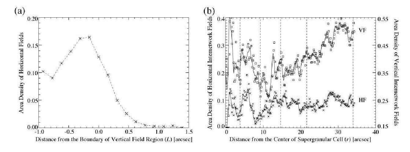
Figure 8 (a) shows the area density of the HFs derived with this procedure. There are more HFs around the boundary of the VF pixels; the area density of the HFs reaches its maximum point at the inward distance of (1 pixel) and rapidly decrease over 06. This clearly shows a remarkable association of the smaller HF patches with the larger VF patches at their borders.

We detect 1085 HF patches in the internetwork region, and 53% of them have circular polarization signals () of both polarities inside the HF patches and their vicinity (within outward distance of one pixel ). The HF patches that have one polarity comprise another 43% of the HF patches. The rest of the HF patches (4%) do not have any circular polarization (). A similar result is reported by Danilovic et al. [7] using the Sunrise/IMax instrument. Horizontal magnetic fields without accompanying vertical components are reported by Jin et al. [23]. Such HFs were found by Jin et al. [23] for 20% of the detectable events, a percentage that is much higher than the one from our own analysis (4%). In our analysis, we chose the pixels for which polarization signals are as weak as possible, yet still have minimal influence from noise. This careful treatment should have enabled us to find a larger number of HF patches without vertical components in the internetwork region if the results of Jin et al. [23] were correct. In Figure 7 (a), HF patches with of both polarities (bipolar HF patches) are shown with red contours, while HF patches with of one polarity (unipolar HF patches) are shown with green contours. The HF patches without (isolated HF patches) are indicated with blue contours.
| Bipolar (574) | Unipolar (467) | Isolated (43) | All (1084) | |||||
| mean | SD | mean | SD | mean | SD | mean | SD | |
| max (Mx cm-2) | 39 | 52 | 47 | 69 | 41 | 58 | ||
| max (Mx cm-2) | 157 | 60 | 112 | 38 | 91 | 24 | 135 | 56 |
| Area (arcsec2) | 0.58 | 0.72 | 0.19 | 0.17 | 0.12 | 0.04 | 0.39 | 0.57 |
IV Properties of horizontal magnetic patches
We investigate whether the properties of the HF patches such as their magnetic flux density, their size, and their locations depend on the presence of the vertical magnetic components. Figure 9 (a) indicates the normalized histograms of the maximum unsigned vertical magnetic flux density inside the HF patch. For bipolar HF patches (red lines), the histogram includes the maximum value of the positive magnetic flux density and that of the unsigned negative magnetic flux density. In the weak end of vertical magnetic flux density (100 Mx cm-2), there is no significant difference between unipolar HF events (green lines) and bipolar ones (red lines). However, more unipolar events harbor relatively strong vertical magnetic flux density ( Mx cm-2). These events would represent the canopy structures of the vertical magnetic elements, and one example is seen in the unipolar HF patch at (27″, 46″) in figure 7 (a).
Figure 9 (b) shows the histogram of the maximum horizontal magnetic flux density in the bipolar (red lines), the unipolar (green), and the isolated HF patches (black). Here the isolated HF patches refer to those without detectable circular polarization signal. The maximum horizontal magnetic flux density of the bipolar HF patches ranges up to 350 Mx cm-2 with an average value of 157 Mx cm-2, while the maximum horizontal magnetic flux density of the unipolar HF patches ranges to 200 Mx cm-2 with an average value of 112 Mx cm-2 (see also table 1). On average, the maximum horizontal flux density of the bipolar HF patches is larger than that of the unipolar HF patches. The flux density of the isolated HF patches is essentially below 150 Mx cm-2 with an average value of 91 Mx cm-2, and is much weaker than that of HF patches associated with a vertical component.
The histograms of the area of these patches are shown in figure 9 (c). The area of the bipolar HF patches distributes over the wide range, while the area of the unipolar HF patches is essentially limited to 1.0 arcsec2 and 74% of the unipolar HF patches are smaller than 0.2 arcsec2. The area of all the isolated events is smaller than 0.2 arcsec2. The number of HF patches generally increases with decreasing size, and about 20 % of the HF patches have a size smaller than 0.1 arcsec2 (4 pix), which is comparable to the SOT/SP spatial resolution (). This indicates that there are a number of HF patches that are not resolved with SOT/SP.
Figure 9 (d) shows the normalized continuum intensity distributions for bipolar and unipolar HF patches, and the VF patches (blue line) in the internetwork region. It appears that the continuum intensity distributions for both bipolar and unipolar HF patches have peaks slightly brighter than that for the whole subfield (dashed line), and are higher than the intensity distribution of the whole subfield at intermediate intensities (0.95 – 1.05). This is consistent with the observations that HF patches are statistically located in the outer boundary of the granules [28, 6, 18, 16, 7]. We do not display the continuum intensity distribution of the isolated HF patches, which is noisy due to the small number of pixels. It appears that (1) the continuum intensity distribution of VF patches has a peak darker than that of the whole subfield, and is higher at the lower intensities (0.85 – ) and that (2) the continuum intensities of VF patches are darker than those of HF patches, and VF patches could be located closer to the intergranular lane.
The unipolar HF events have lower horizontal magnetic flux densities, and a smaller area than the bipolar events. Both bipolar and unipolar events tend to be located in the periphery of granules. As to the isolated HF patches, the horizontal magnetic flux densities are low and their areas are small compared with the bipolar and unipolar HF patches. Although some unipolar HF patches correspond to the canopy structures of the vertical magnetic fields, it is conceivable that the some unipolar and isolated HF patches are essentially the same phenomena as the bipolar patches; they have the loop structure with bipolar footpoints. Since the sensitivity to horizontal field is low compared with sensitivity to the vertical field, only cores of the HF patches attached to one of the footpoints are detected as unipolar HF patches. This would result in the smaller size of the unipolar HF patches. The candidate for such HF patches is found at (25″, 43″) in figure 7 (a). When the HF patches have a size closer to the resolution element of the telescope, their circular polarization signals with opposite polarities corresponding to their footpoints start to be canceled out. As a result, the residual Stokes signal becomes weak, and it is possible that only circular polarization signals with one dominant polarity are left, or all the Stokes signals are completely canceled out.



V Estimation of horizontal and vertical magnetic fluxes
V.1 Global magnetic flux balance of VF and HF patches
In this section, we compare the total magnetic fluxes to clarify which component dominates the internetwork region, vertical or horizontal. We derive and compare the total vertical and horizontal magnetic flux in the pure internetwork region. In figure 6 (c), the cross mark indicates the center position of a supergranular cell, and we define the region within a distance of from the center (orange circle) as the pure internetwork region. Some vertical patches crossing over the orange line are also included in the analysis. We consider the HF patches that are located inside the orange circle and overlap with the VF patches (dark blue contours in figure 6 (c)). The VF patches without HFs are shown with the light blue contours in figure 6 (c).
The total unsigned vertical magnetic flux within the orange circle is given by , where is the intrinsic magnetic field strength, the filling factor, the scanning step size of , and is the pixel scale along the slit of 016. The total flux is estimated to be 3.01019 Mx cm-2 and the average flux density is 8.3 Mx cm-2. If we consider only the VF patches that have the HF patches, total vertical magnetic flux is estimated to be 2.71019 Mx cm-2, and the average flux density is 7.5 Mx cm-2. We reach the remarkable conclusion that most (91%) of the vertical magnetic flux are contributed by the VF patches accompanied by the HF patches. The mean flux density obtained here is comparable to the one obtained by Orozco Suárez et al. [39, 9.5 Mx cm-2] and Lites et al. [28, 11.7 Mx cm-2].
Following Lites et al. [28], we also derive the spatial average horizontal flux density defined by , where is the total area enclosed by the orange circle. The average horizontal flux density is 7.1 Mx cm-2 which is comparable to the vertical one derived above and much smaller than the one obtained by Lites et al. [28, 60 Mx cm-2].
Unlike the VF case, the horizontal magnetic flux cannot be estimated by times the pixel area, since the magnetic fields are directed perpendicular to the LOS. If all the identified horizontal magnetic patches have a flux tube structure [19], the cross section of the individual flux tubes instead of the apparent size should be used for the estimation of the total magnetic flux, where is the lateral size of the flux tube and the thickness along the LOS. Assuming that the flux tube is spatially resolved and the magnetic filling factor is the fraction occupied by the magnetized plasma along the LOS in the line-forming layer, the total magnetic flux of an individual event is estimated by , where is the average horizontal intrinsic field strength in the HF patch and is the length of the line forming region (300 km). Using equation (6), the total magnetic flux is written as , where is the average transverse (horizontal) magnetic flux density in the HF patch. Since is not derived in our analysis, we use the average filling factor of the HFs in the quiet Sun obtained with Milne-Eddington inversion [15]. We fit a spatial ellipse to all the HF patches and use the minor axes for the lateral size of the flux tube . The total magnetic flux of the HF patches within the orange circle taking into account their cross sections is estimated to be 4.71018 Mx. This value is smaller than the total unsigned vertical magnetic flux (3.01019 Mx) by a factor of 6. Since the positive and negative magnetic flux are grossly balanced inside the orange circle, total magnetic flux for the VF patches will be three times larger than that for the HF patches. This value could be larger or smaller, since we assume the nominal filling factor of 0.15 and the thickness of the line-forming layer of 300 km, and roughly estimate the cross section of the flux tubes.
V.2 Local magnetic flux balance of VF and HF patches
Given the fact that the HF patches are closely associated with the VF patches (Section III), we quantitatively examine the magnetic flux of the VF patches associated with each HF patch. We estimate the magnetic flux of the HF patches by considering the cross section of the flux tubes as was done in Section V.1. We identify the overlapping HF and VF patches, and plot the ratio of HF and VF fluxes in figure 10. There are cases where an individual HF patch overlaps with several VF patches, and vice versa. If the VF magnetic flux is larger than the HF flux, we take the ratio of the VF flux to the HF flux (solid line in figure 10). If the HF flux is larger than the VF flux, we take the ratio of the HF flux to the VF flux (dashed line in figure 10). The histograms in figure 10 have the peak at 1, indicating that the magnetic fluxes of associated HF and VF patches are well balanced.

VI Intrinsic Magnetic Field Strength
In this section, we examine the Stokes amplitude line ratio to infer intrinsic field strength [51]. Figure 11 shows the scatter plots of the maximum Stokes amplitudes in the blue lobe of Fe I 630.15 nm and 630.25 nm lines. We measure the line ratio of the the pixels inside the orange circle shown in the figure 6 (c). If the intrinsic field strengths are much weaker than 1 kG, the Stokes is proportional to , where is the Landé factor (, ) . In this case, we expect the data points to regress to the dashed line in figure 11. The slope of the dashed line is given by,
| (8) |
The value of the slope is based on the global averages over all the pixels in the analyzed subfield of the maximum amplitudes of in the blue lobe of Fe I 630.15 nm and 630.25 nm lines.
The data points of the VF pixels inside the HF patches are clearly concentrated along the line with the slope of (figure 11 (a)). Where the VF pixels do not overlap with the HF patches, most of data points remain around the dashed line. However, some points with larger Stokes amplitudes start to bend away from this line, and follow the line with the slope of 0.7, shown with the solid line (black contours in figure 11 (b)). This transition is due to the differential Zeeman saturation for stronger fields between two Fe I 630.2 lines, and the slope of indicates the field strength of order of 1 kG [51].
Figure 11 (c) shows the scatter plot for the network fields indicated with yellow contours in figure 6 (b). The points are completely away from the line with the slope , and regress to the line with the slope of 0.7 (solid line) and 0.6 for higher Stokes signal. The coefficients of 0.6 and 0.7 are given by Stenflo [51] for the strong saturated intrinsic field strength. This scatter plot clearly indicates that the network region consists of strong kG fields. These strong kG vertical fields located in the internetwork region would be formed by convective collapse [40, 13, 37, 11, 51].

VII Spatial distribution internetwork magnetic fields on the supergranular scale
In this section, we qualitatively examine the spatial distributions of the internetwork horizontal and vertical magnetic fields on the supergranular scale, and aim to address the question of whether the supergranulation affects the distribution of these small-scale internetwork fields.
The area density of the VF patches at a distance from the center position of the supergranular cell (cross mark in figure 6 (d)) is given by
| (9) |
where, at a distance between and , is the total number of pixels, and the number of pixels occupied by the VF patches. Here we take pixel (). When we obtain and , we do not take into account the network pixels marked with yellow contours. Likewise, the area density of HFs is given by
| (10) |
where is the total number of the HF pixels marked with red contours at a distance between and from the center position of the supergranular cell.
Figure 8 (b) shows the area density and . Five dashed lines indicate and , and correspond to the orange circle () in figure 6 (c) and four circles in figure 6 (d). We find a significant difference in the spatial distributions between the HF and VF patches. The area density of the VF patches, , increases with distance. Meanwhile, the area density of the HF patches does not change from the center to the network boundary, and this clearly shows that the HF distribution does not have any correlation with the supergranular scale.
VIII Discussion
VIII.1 Spatial coincidence of VF and HF patches
One of the discoveries presented in this paper is the clear positional association of the VF and HF patches in the internetwork region. The HF patches are located around the boundary of the VF patches as shown in Figure 8 (a), and are connected to the VF patches. of the total number of the HF patches has the associated VF patches, and 70% of the total area occupied by the HF patches overlaps with the VF patches. Alternatively, 49% of the total number of the VF patches has the HF patches. The size of the HF patches are apparently smaller compared to that of the VF patches as shown in figure 6 (a). Only the small core of the HF patches may be seen due to the lower sensitivity of the linear polarization to the magnetic field strength. We quantitatively compare the individual VF flux with the flux of the corresponding HF patch, and find that the VF flux is close to the HF flux (figure 10). The HF patches so far have been investigated by many authors as a new magnetic entity different from the vertical internetwork fields. However, they are closely connected, possibly causally related to the well-known VF patches in the internetwork regions. The implication of this observational fact will be discussed in the subsequent sections.
As shown in figure 8 (b), the area densities of both the HF and VF patches are essentially constant within . This is consistent with the observation that the VF and HF patches are closely connected. The area density of the HF patches stays the same with radius from the center of the supergranule, while that of the VF patches gradually increases closer to the supergranular boundary. This behavior at is apparently different from the correspondence between the HF and VF patches in the pure internetwork region. Apparent large-size network fields indicated with yellow contours in figure 6 (b) are not included in figure 8 (b). The histogram of the intrinsic field strengths and the occurrence rates of horizontal fields are the same between the quiet Sun and the weak plage region when the strong persistent vertical fields (network fields) are removed [15]. Furthermore, the histograms of the intrinsic field strengths are the same between the quiet Sun near the equatorial limb and the polar region after removing the vertical fields including the network fields [22]. The distributions of the HF and VF patches in figure 8 (b) are consistent with the earlier results by Ishikawa & Tsuneta [15] and Ito et al. [22].
VIII.2 Comparison of longitudinal and transverse apparent flux density
We estimate and compare the total magnetic flux for both VF and HF patches in the internetwork region. The mean flux density for unsigned longitudinal (vertical) component is estimated to be 8.3 Mx cm-2 and the mean apparent flux density for transverse (horizontal) component is 7.1 Mx cm-2. We do not find the significant imbalance between them as reported by Lites et al. [28]. As seen in figure 2, we expect that the photon noise contaminates the real signal within or , making it difficult to distinguish the real signals from the noise. Thus, we exclude these pixels and calculate the mean apparent flux density. On the other hand, Lites et al. [28] used all the pixels for the determination of the mean apparent flux densities in the FOV; their noise levels are 2.4 Mx cm-2 and 41 Mx cm-2 for the longitudinal and transverse apparent flux densities.
The total unsigned vertical magnetic flux in the internetwork region defined by the orange circle in figure 6 (c) is estimated to be 3.0 Mx. In order to accurately estimate the total magnetic flux density for the HF patches in the internetwork region, we consider that all the HF patches have the flux tube structure as shown in Ishikawa et al. [19], and take into account the cross section of the each horizontal flux tube. Indeed, the HF patches are considered to be a manifestation of the small-scale bipolar flux tubes as discussed at the end of section IV.
The estimated total magnetic flux of the HF patches is 4.7 Mx, which is smaller than that of the VF patches. One reason for this difference may be different sensitivity between Stokes in detecting the longitudinal (VF) component and Stokes in detecting the transverse (HF) component. If emerging loops leave the photosphere, there should be more leftover vertical flux, which corresponds to the footpoints of these loops, than the horizontal flux. This is both possible and plausible to have more vertical flux in addition to the sensitivity issue. Indeed, it is observed that some small-scale loops emerge and reach above the photosphere, leaving behind the bipolar footpoints [34, 19].
VIII.3 Origin of internetwork fields
Isobe et al. [21] and Steiner et al. [49] carried out the numerical simulation of the surface layer of the Sun having an initial condition of vertical unipolar magnetic fields. They then compared the simulation with observations. Their initialization is similar to plage and network regions where vertical fields are dominant. They found that the initially uniform magnetic fields are immediately bent by the convective flows, and they eventually become disordered due to the convective motion and appear as horizontal fields in the photosphere. Steiner et al. [49] also carried out the simulation initialized with uniform horizontal magnetic fields, and found that the amount of granular-scale horizontal fields exceeds that of the initialization with uniform unipolar magnetic fields.
We find that the area density of the HF patches does not increase toward the supergranular boundary, even though the area density of the VF patches increases toward the supergranular boundary. This independence of the HF patches from the amount of the VF patches indicates that the seed fields for the HF patches do not come from the pre-existing vertical magnetic fields, and our observations appear not to be consistent with the initialization with a unipolar vertical magnetic field that Isobe et al. [21] and Steiner et al. [49] used. Although we cannot rule out other possibilities for the origin of the horizontal magnetic fields, it would be conceivable that the granular convective motions amplify the field strength of the seed fields up to the equipartition field strength corresponding to the granular motion by stretching and folding, and drive the emergence of the horizontal magnetic fields from the convection zone.
VIII.4 Origin of kG vertical magnetic fields
Measuring the Stokes line ratio of the Fe I 630.15/630.25 system [51], we obtain the intrinsic field strength in an internetwork region. The intrinsic field strength inside the HF patches is dominantly weak ( kG), and is in the regime of the weak field approximation. Most of the pixels outside the HF patches (but located inside the VF patches) also have weak intrinsic field strength, but a significant population of strong (kG) fields may also be seen for those regions (figure 11 (b)). Such signature of kG intrinsic fields cannot be found inside the HF patches, as clearly shown in figure 11 (a). The intrinsic field strength in the designated network region is completely above 1 kG (figure 11 (c)).
We point out that the observed weak intrinsic field strength inside the HF patches is in the sub-equipartition regime of the magnetic fields strength. The equipartition field strength corresponding to the granular convection is estimated to be 700 G, where the density is g cm-3 at a depth of 500 km below the surface and the velocity is 2 km s-2. On the other hand, some pixels outside the HF patches have field strength above the equipartition value.
As shown in figure 9 (d) the HF patches are statistically located inside the granular cells, while the VF patches in the internetwork regions prefer to be located in the darker region, i.e., closer to the intergranular lanes, though there is a large spread in intensity. We conjecture that the magnetic fields below or equal to the equipartition field strength are provided by the emergence of granular-scale horizontal fields. When the emerged flux tubes successfully leave the photosphere with left-over footpoints (vertical flux tube), the footpoints are intensified beyond the equipartition field strength (super-equipartition field strength of 1-2 kG) due to convective instability. We interpret that the scatter plot of figure 11 (b) shows such evolutionary process from sub-equipartition to super-equipartition fields: outer higher loops have the photospheric footpoints (VF patches) without the HF patches, since the top of such loops has already left the photosphere. We speculate that such vertical fields corresponding to the VF patches may remain in the sub-equipartition regime, or may be subsequently subject to convective collapse, resulting in kG-vertical fields. Alternatively, the footpoints of the HF patches may almost immediately become strong (super-equipartition) vertical fields due to convective collapse when the HF patches are advected by the granular flows to the intergranular lanes.
Nagata et al. [37] found the observational evidence of the formation of kG flux tube induced by convective collapse using SOT/SP [11, see also ]; an equipartition field strength flux tube with the preceding transient downflow of 6 km s-1 goes through the intensification of the field strength to 2 kG. The strong downward flow comparable to the local sound speed is observed in the footpoint region of the small-scale emerging horizontal fields, suggesting the occurrence of convective collapse at the footpoints of horizontal fields [18]. However, we point out that there is no direct piece of evidence that all the kG vertical magnetic fields in the internetwork region come from the emergence of horizontal magnetic fields. Further investigations have to be done.
VIII.5 Do horizontal fields concentrate on the supergranular boundary?
The appearance of the transient horizontal magnetic fields is not spatially random, and has an organized cellular structure with a typical scale of 5-10. The cellular structures coincide in position with the negative divergence of the horizontal flow field, i.e., mesogranular boundaries with downflows [17]. As for the internetwork vertical fields, a similar concentration has been observed [10]. Indeed, both the HF and VF patches concentrate in the cellular structure with a scale of 5-10 in the snapshot image of figure 6 (a). These structures would correspond to the mesogranular cells. A natural question here is whether there is a similar concentration of horizontal magnetic fields in the supergranular boundaries. We find that the area density of the VF patches increases toward the supergranular boundary, while the area density of the HF patches is essentially constant with distance. The HF patches are not concentrated on the supergranular boundary.
The horizontal flow velocity of the supergranulation at the photosphere is in the range 300-500 m s-1 [46]. Collapsed vertical fields (Section VIII.4) can be advected by the supergraular flow fields, and might form the network fields around the supergranular boundaries. The abundant vertical fields around the supergranular boundary might be originally provided by the emergence of the horizontal fields in the internetwork region.
Martin [32] and Schrijver et al. [44] pointed out that the main source of the network magnetic fields are the ephemeral region and that the contribution of the internetwork magnetic fields is not so significant [56, see also]. The ephemeral region consists of the emerging bipolar magnetic patches with a size less than . We find that the internetwork region is filled with a lot of small-scale emerging bipolar magnetic fields, which are not clearly seen with the previous generation telescope. The relationship between the ephemeral region and the transient horizontal magnetic fields needs to be clarified.
Here we speculate that vertical magnetic fields in the internetwork fields are advected by the supergranular horizontal flow and that the network fields would be formed. Using Hinode/SOT observation, de Wijn et al. [9] find that apparent flow velocities of magnetic elements (patches) in the internetwork region are slightly biased by 0.2 km s-1 in a radial direction toward the network boundary. It is clear that the motion of the internetwork magnetic patches is affected by the supergranular flow fields. However, there is no direct evidence showing that the network magnetic fields are a consequence of the accumulation of the internetwork magnetic fields. In order to confirm that the internetwork fields are indeed advected towards the supergranular boundaries forming the network fields, further investigation needs to be done with the high spatial and temporal resolution observations using Hinode/SOT.
Ishikawa & Tsuneta [17] point out that the seed fields of the horizontal fields are advected by the mesogranular flow fields, and granular convective motion amplifies the field strength from below the mesogranular equipartition field strength to granular , and drives the emergence of the horizontal fields. If the seed fields are advected by the mesogranular flow fields, the seed fields are also likely to be advected by the supergranular flow: we should have seen the concentration of the horizontal fields around the supergranular boundaries. We do not have a clear interpretation for this asymmetry between mesogranule and supergranule in terms of the population of the HF patches. This issue would be related to a fundamental relationship between the small-scale magnetic fields and the convection with different scale sizes.
IX Summary and Speculation
In the present paper, we have analyzed the high spatial resolution spectropolarimetric data obtained with the SOT/SP to investigate the properties of the internetwork magnetic fields. We have paid special attention to the effect of the photon noise in the analyzed data, and chosen the valid pixels minimally contaminated by the noise. Therefore, the present paper is limited in scope to the field with sufficiently strong polarization signal. An obvious penalty of having the stringent noise criteria is that we do not detect weak magnetic fields which provide polarization signal comparable to or weaker than the noise level. We do not rule out the existence of such weak fields. We refer the pixels with the significant Stokes signal to the VF (vertical field) pixels, and those with the significant Stokes or to the HF (horizontal field) pixels. The main observational results with our immediate interpretation are summarized as follows:
- 1.
We find positional association between the vertical and the horizontal magnetic fields in the internetwork region. The vertical magnetic fields correspond to the weak vertical magnetic fields known for decades to exist. The horizontal magnetic fields are investigated in detail with Hinode for the first time. Approximately half of the total number of the VF patches accommodates the HF patches partially or entirely, and essentially all of the HF patches overlap with the VF patches. These HF patches are typically located around the edge of the VF patches. We compare the VF flux with the flux of the corresponding HF patch, and find that HF flux is close to the VF flux. These observations suggest that the HF patches are physically and causally connected to the VF patches in the internetwork region. It has been discussed that the transient horizontal magnetic fields are a manifestation of the local dynamo process [15, 22]. The origin of the vertical magnetic fields in the internetwork region is not yet known, and this positional coincidence may allow us to reach a unified understanding of the internetwork fields in general.
- 2.
Approximately half of the HF patches have bipolar patches (Stokes signals), and the other half have the unipolar Stokes signal. The unipolar HF patches have both a smaller size and smaller horizontal magnetic flux densities. We suggest that only dominant polarity is seen due to the cancellation of the Stokes signal within the resolution element in the unipolar HF patches, and that the HF patches have an essentially bipolar structure. Another possibility is that a small portion of the bipolar HF patches may be detected as unipolar HF patches.
- 3.
The mean longitudinal (vertical) magnetic flux density is estimated to be 8.3 Mx cm-2, and the apparent transverse (horizontal) one is 7.1 Mx cm-2. The former number is close to the one derived in the previous studies [39, 28, e.g.,], but the apparent transverse flux density derived here is a factor of 5 smaller than the one obtained by Lites et al. [28]. In our analysis, the mean magnetic flux density of the vertical fields is almost the same as that of the horizontal fields. We also estimate the total magnetic flux of the HF patches, taking into account the cross section of the horizontal flux tubes, and find that the total magnetic flux of the HF patches is a factor of 3 smaller than that of the VF patches. This excess of the total magnetic flux of the VF patches would indicate that the some portion of the vertical fields inside the VF patches reach above the photosphere.
- 4.
Measuring the Stokes polarization of the Fe I 630.15-630.25 nm line system (line ratio method; Stenflo [50]), we infer the intrinsic field strength in the internetwork region. The intrinsic field strengths inside the HF patches (overlapping area of the VF and HF patches) are weak ( kG), while the strengths outside the HF patches (non-overlapping area) range from weak to strong (kG). This would suggest that convective collapse takes place at the footpoint (vertical portion) of the emerging horizontal field that is about to leave or that has left the line-forming region in the photosphere, and this is considered to be one of the mechanisms to produce strong (kG) fields in the internetwork region. The two distinct flux populations represent the pre-collapsed and the post-collapsed vertical flux tubes [51]. The snapshot image analyzed in this paper contains the two evolutionary states.
- 5.
It is well known that the VF patches concentrate on the mesogranular and supergranular boundaries, while we show in this paper that the HF patches concentrate only on the mesogranular boundaries of the supergranunlar cell studied here. Only the VF patches concentrate around the supergranular boundary. In the internetwork region within from the center position of the supergranulation, the area densities of both VF and HF patches are constant with radius. The area density of only VF patches increases with increasing radius outside radius (closer to the network boundary). The area density of HF patches does not increase even though there are more VF patches closer to the supergranular boundary, and this independence of the amount of the HF patches suggests that the HF patches are not due to the bending of pre-existing vertical magnetic fields with the granular convective motion [21].
These observations shed light on the origins of both the vertical and horizontal magnetic fields and their causal relationship, potentially leading to a new picture on the quiet Sun magnetism. As a first step for a unified understanding on the quiet Sun magnetism, we here proposed one possible scenario for generation and maintenance of the internetwork vertical and horizontal magnetic fields: (1) mesogranular flow fields may advect the seed fields with field strength smaller than mesogranular into the mesogranular boundaries. The granular convective motion amplifies the field strength of the seed fields up to granular by folding and stretching, and the granular upward motion carries them to the photosphere. These are observed as the small-scale horizontal magnetic fields on the photosphere. This process is discussed in Ishikawa & Tsuneta [17]. (2) Some horizontal fields reach above the photosphere, leaving their footpoints (bipolar magnetic fields). (3) Vertical magnetic fields, which are the footpoints of the emerged small-scale loops, are advected toward the intergranular lane, and are subject to convective collapse, partially forming strong kG fields. (4) Finally, these vertical fields are transported to the supergranular boundaries, and form the network magnetic fields.
The occurrence rate of the emergence of the horizontal magnetic fields is quite high [15]. It is likely that such horizontal fields do not return to the photosphere and that they reach the chromosphere and possibly corona [34, 19]. It is found that 23% of the small-scale loops on the photosphere reach above the line forming region of Fe I 630.2 nm lines [34], and the total magnetic flux carried by the horizontal magnetic fields above the photosphere is estimated to be two orders of magnitude larger than the total magnetic flux of the sunspots [23, 19]. The rest of them would be shredded, thus falling below the threshold of detectability, and/or return below the photosphere. It is plausible that the emergence of these ubiquitous small-scale loops leaves the vertical magnetic fields on the photosphere, and is the source of the quiet Sun magnetic fields with the process suggested above.
References
- [1] Asensio Ramos, A. 2009, ApJ, 701, 1032
- [2] Barthol, P., Gandorfer, A., Solanki, S. K., Schüssler, M., Chares, B., Curdt, W., Deutsch, W., Feller, A., Germerott, D., Grauf, B., Heerlein, K., Hirzberger, J., Kolleck, M., Meller, R., Müller, R., Riethmüller, T. L., Tomasch, G., Knölker, M., Lites, B. W., Card, G., Elmore, D., Fox, J., Lecinski, A., Nelson, P., Summers, R., Watt, A., Martínez Pillet, V., Bonet, J. A., Schmidt, W., Berkefeld, T., Title, A. M., Domingo, V., Gasent Blesa, J. L., del Toro Iniesta, J. C., López Jiménez, A., Álvarez-Herrero, A., Sabau-Graziati, L., Widani, C., Haberler, P., Härtel, K., Kampf, D., Levin, T., Pérez Grande, I., Sanz-Andrés, A., & Schmidt, E. 2010, ArXiv e-prints
- [3] Beck, C. & Rezaei, R. 2009, A&A, 502, 969
- [4] Bommier, V., Martínez González, M., Bianda, M., Frisch, H., Asensio Ramos, A., Gelly, B., & Landi Degl’Innocenti, E. 2009, A&A, 506, 1415
- [5] Cattaneo, F. 1999, ApJ, 515, L39
- [6] Centeno, R., Socas-Navarro, H., Lites, B., Kubo, M., Frank, Z., Shine, R., Tarbell, T., Title, A., Ichimoto, K., Tsuneta, S., Katsukawa, Y., Suematsu, Y., Shimizu, T., & Nagata, S. 2007, ApJ, 666, L137
- [7] Danilovic, S., Beeck, B., Pietarila, A., Schüssler, M., Solanki, S. K., Martínez Pillet, V., Bonet, J. A., del Toro Iniesta, J. C., Domingo, V., Barthol, P., Berkefeld, T., Gandorfer, A., Knölker, M., Schmidt, W., & Title, A. M. 2010, ApJ, 723, L149
- [8] De Pontieu, B. 2002, ApJ, 569, 474
- [9] de Wijn, A. G., Lites, B. W., Berger, T. E., Frank, Z. A., Tarbell, T. D., & Ishikawa, R. 2008, ApJ, 684, 1469
- [10] Domínguez Cerdeña, I. 2003, A&A, 412, L65
- [11] Fischer, C. E., de Wijn, A. G., Centeno, R., Lites, B. W., & Keller, C. U. 2009, A&A, 504, 583
- [12] Harvey, J. W., Branston, D., Henney, C. J., Keller, C. U., & SOLIS and GONG Teams. 2007, ApJ, 659, L177
- [13] Hasan, S. S. 1985, A&A, 143, 39
- [14] Ichimoto, K., Lites, B., Elmore, D., Suematsu, Y., Tsuneta, S., Katsukawa, Y., Shimizu, T., Shine, R., Tarbell, T., Title, A., Kiyohara, J., Shinoda, K., Card, G., Lecinski, A., Streander, K., Nakagiri, M., Miyashita, M., Noguchi, M., Hoffmann, C., & Cruz, T. 2008, Sol. Phys., 249, 233
- [15] Ishikawa, R. & Tsuneta, S. 2009a, A&A, 495, 607
- [16] Ishikawa, R. & Tsuneta, S. 2009b, in Astronomical Society of the Pacific Conference Series, Vol. 415, Astronomical Society of the Pacific Conference Series, ed. B. Lites, M. Cheung, T. Magara, J. Mariska, & K. Reeves, 132–139
- [17] —. 2010, ApJ, 718, L171
- [18] Ishikawa, R., Tsuneta, S., Ichimoto, K., Isobe, H., Katsukawa, Y., Lites, B. W., Nagata, S., Shimizu, T., Shine, R. A., Suematsu, Y., Tarbell, T. D., & Title, A. M. 2008, A&A, 481, L25
- [19] Ishikawa, R., Tsuneta, S., & Jurčák, J. 2010, ApJ, 713, 1310
- [20] Ishikawa, R., Tsuneta, S., Kitakoshi, Y., Katsukawa, Y., Bonet, J. A., Vargas Domínguez, S., Rouppe van der Voort, L. H. M., Sakamoto, Y., & Ebisuzaki, T. 2007, A&A, 472, 911
- [21] Isobe, H., Proctor, M. R. E., & Weiss, N. O. 2008, ApJ, 679, L57
- [22] Ito, H., Tsuneta, S., Shiota, D., Tokumaru, M., & Fujiki, K. 2010, ApJ, 719, 131
- [23] Jin, C., Wang, J., & Zhou, G. 2009, ApJ, 697, 693
- [24] Khomenko, E. V., Collados, M., Solanki, S. K., Lagg, A., & Trujillo Bueno, J. 2003, A&A, 408, 1115
- [25] Kosugi, T., Matsuzaki, K., Sakao, T., Shimizu, T., Sone, Y., Tachikawa, S., Hashimoto, T., Minesugi, K., Ohnishi, A., Yamada, T., Tsuneta, S., Hara, H., Ichimoto, K., Suematsu, Y., Shimojo, M., Watanabe, T., Shimada, S., Davis, J. M., Hill, L. D., Owens, J. K., Title, A. M., Culhane, J. L., Harra, L. K., Doschek, G. A., & Golub, L. 2007, Sol. Phys., 243, 3
- [26] Lin, H. 1995, ApJ, 446, 421
- [27] Lin, H. & Rimmele, T. 1999, ApJ, 514, 448
- [28] Lites, B. W., Kubo, M., Socas-Navarro, H., Berger, T., Frank, Z., Shine, R., Tarbell, T., Title, A., Ichimoto, K., Katsukawa, Y., Tsuneta, S., Suematsu, Y., Shimizu, T., & Nagata, S. 2008, ApJ, 672, 1237
- [29] Lites, B. W., Leka, K. D., Skumanich, A., Martinez Pillet, V., & Shimizu, T. 1996, ApJ, 460, 1019
- [30] Lites, B. W., Rutten, R. J., & Berger, T. E. 1999, ApJ, 517, 1013
- [31] Livingston, W. & Harvey, J. 1971, in IAU Symposium, Vol. 43, Solar Magnetic Fields, ed. R. Howard, 51
- [32] Martin, S. F. 1990, in IAU Symposium, Vol. 138, Solar Photosphere: Structure, Convection, and Magnetic Fields, ed. J. O. Stenflo, 129
- [33] Martínez González, M. J., Asensio Ramos, A., López Ariste, A., & Manso Sainz, R. 2008, A&A, 479, 229
- [34] Martínez González, M. J. & Bellot Rubio, L. R. 2009, ApJ, 700, 1391
- [35] Martinez Pillet, V., del Toro Iniesta, J. C., Alvarez-Herrero, A., Domingo, V., Bonet, J. A., Gonzalez Fernandez, L., Lopez Jimenez, A., Pastor, C., Gasent Blesa, J. L., Mellado, P., Piqueras, J., Aparicio, B., Balaguer, M., Ballesteros, E., Belenguer, T., Bellot Rubio, L. R., Berkefeld, T., Collados, M., Deutsch, W., Feller, A., Girela, F., Grauf, B., Heredero, R. L., Herranz, M., Jeronimo, J. M., Laguna, H., Meller, R., Menendez, M., Morales, R., Orozco Suarez, D., Ramos, G., Reina, M., Ramos, J. L., Rodriguez, P., Sanchez, A., Uribe-Patarroyo, N., Barthol, P., Gandorfer, A., Knoelker, M., Schmidt, W., Solanki, S. K., & Vargas Dominguez, S. 2010, ArXiv e-prints
- [36] Moreno-Insertis, F., Caligari, P., & Schuessler, M. 1995, ApJ, 452, 894
- [37] Nagata, S., Tsuneta, S., Suematsu, Y., Ichimoto, K., Katsukawa, Y., Shimizu, T., Yokoyama, T., Tarbell, T. D., Lites, B. W., Shine, R. A., Berger, T. E., Title, A. M., Bellot Rubio, L. R., & Orozco Suárez, D. 2008, ApJ, 677, L145
- [38] Orozco Suárez, D., Bellot Rubio, L. R., Del Toro Iniesta, J. C., Tsuneta, S., Lites, B., Ichimoto, K., Katsukawa, Y., Nagata, S., Shimizu, T., Shine, R. A., Suematsu, Y., Tarbell, T. D., & Title, A. M. 2007a, PASJ, 59, 837
- [39] Orozco Suárez, D., Bellot Rubio, L. R., del Toro Iniesta, J. C., Tsuneta, S., Lites, B. W., Ichimoto, K., Katsukawa, Y., Nagata, S., Shimizu, T., Shine, R. A., Suematsu, Y., Tarbell, T. D., & Title, A. M. 2007b, ApJ, 670, L61
- [40] Parker, E. N. 1978, ApJ, 221, 368
- [41] Ploner, S. R. O., Schüssler, M., Solanki, S. K., & Gadun, A. S. 2001, in Astronomical Society of the Pacific Conference Series, Vol. 236, Advanced Solar Polarimetry – Theory, Observation, and Instrumentation, ed. M. Sigwarth, 363
- [42] Ruiz Cobo, B. & del Toro Iniesta, J. C. 1992, ApJ, 398, 375
- [43] Sanchez Almeida, J. 1997, ApJ, 491, 993
- [44] Schrijver, C. J., Title, A. M., van Ballegooijen, A. A., Hagenaar, H. J., & Shine, R. A. 1997, ApJ, 487, 424
- [45] Shimizu, T., Nagata, S., Tsuneta, S., Tarbell, T., Edwards, C., Shine, R., Hoffmann, C., Thomas, E., Sour, S., Rehse, R., Ito, O., Kashiwagi, Y., Tabata, M., Kodeki, K., Nagase, M., Matsuzaki, K., Kobayashi, K., Ichimoto, K., & Suematsu, Y. 2008, Sol. Phys., 249, 221
- [46] Shine, R. A., Simon, G. W., & Hurlburt, N. E. 2000, Sol. Phys., 193, 313
- [47] Socas-Navarro, H. & Lites, B. W. 2004, ApJ, 616, 587
- [48] Solanki, S. K., Barthol, P., Danilovic, S., Feller, A., Gandorfer, A., Hirzberger, J., Riethmüller, T. L., Schüssler, M., Bonet, J. A., Martínez Pillet, V., del Toro Iniesta, J. C., Domingo, V., Palacios, J., Knölker, M., Bello González, N., Berkefeld, T., Franz, M., Schmidt, W., & Title, A. M. 2010, ApJ, 723, L127
- [49] Steiner, O., Rezaei, R., Schaffenberger, W., & Wedemeyer-Böhm, S. 2008, ApJ, 680, L85
- [50] Stenflo, J. O. 1973, Sol. Phys., 32, 41
- [51] —. 2010, A&A, 517, A37
- [52] Suematsu, Y., Tsuneta, S., Ichimoto, K., Shimizu, T., Otsubo, M., Katsukawa, Y., Nakagiri, M., Noguchi, M., Tamura, T., Kato, Y., Hara, H., Kubo, M., Mikami, I., Saito, H., Matsushita, T., Kawaguchi, N., Nakaoji, T., Nagae, K., Shimada, S., Takeyama, N., & Yamamuro, T. 2008, Sol. Phys., 249, 197
- [53] Tsuneta, S., Ichimoto, K., Katsukawa, Y., Lites, B. W., Matsuzaki, K., Nagata, S., Orozco Suárez, D., Shimizu, T., Shimojo, M., Shine, R. A., Suematsu, Y., Suzuki, T. K., Tarbell, T. D., & Title, A. M. 2008a, ApJ, 688, 1374
- [54] Tsuneta, S., Ichimoto, K., Katsukawa, Y., Nagata, S., Otsubo, M., Shimizu, T., Suematsu, Y., Nakagiri, M., Noguchi, M., Tarbell, T., Title, A., Shine, R., Rosenberg, W., Hoffmann, C., Jurcevich, B., Kushner, G., Levay, M., Lites, B., Elmore, D., Matsushita, T., Kawaguchi, N., Saito, H., Mikami, I., Hill, L. D., & Owens, J. K. 2008b, Sol. Phys., 249, 167
- [55] Viticchié, B., J., Almeida, S., Del Moro, D., & Berrilli, F. 2010, ArXiv e-prints
- [56] Wang, H. & Zirin, H. 1987, Sol. Phys., 110, 281