Precision cosmology and data
Abstract
At variance from , and abundances, abundance data yield an extra constraint to cosmological parameters, in top of those deriving from CMB, BAO, SNIa or data. This constraint, often disregarded, would favor smaller values, also indicating a preference for Dark Energy state equations well in the phantom regime, simultaneously softening the upper limit on the sum of neutrino masses, up to eV.
Keywords
Dark energy theory, dark matter, cosmological neutrinos, neutrino properties, cosmology of theories beyond the SM1 Introduction
Big-Bang Nucleosynthesis (BBN) is a pillar of evolutionary cosmology. It is however known that “precision” cosmology is not in complete agreement with BBN predictions on ( baryon density parameter, Hubble parameter in units of 100 (km/s)/Mpc ). Agreement is however recovered if abundance data are disregarded.
is the heaviest and most scanty nuclide considered in BBN, but the reaction network leading to is hardly questionable, while its abundance data, resumed in the next Section, are sound. It seems therefore significant to debate what changes in cosmological parameter estimates if abundance data are taken on the same foot as other nuclides.
BBN aims at predicting the abundances of , , , and in terms of a single parameter:
| (1) |
Here and are baryon and CMB photons number densities, respectively. Owing to baryon conservation and assuming no substantial entropy input between BBN and today, their ratio has not changed since then. Data on nuclide abundances will be taken here from recent review papers by Matteucci [1] and Iocco et al. [2], while the network of reactions used for predictions is accurately illustrated in [2].
Tests will be based on WMAP7 data [3]. We shall re-analyse them by using the CosmoMC routines [4] to gauge model likelihood. Together with CMB data, Baryon Acoustic Oscillation (BAO) data [5], as well as either [6] or SNIa data [7], as suitably specified, will be considered.
Our analysis will focus on the Dark Energy (DE) state equation, however assumed to take a scale independent value . Neutrino masses will be considered through the parameter and neglecting their mass hierarchy. A Friedmann-Lemaître-Robertson-Walker metric is assumed, with flat space section.

2 A quick review on stellar abundance
The history of primordial abundance determination starts from the discovery of the Spite & Spite plateau [8]. They found that the abundance, when the warmest metal-poor dwarfs were considered, exhibited no appreciable metallicity dependence, suggesting then a primordial value . Here , being the ratio of number densities.
Recent data, using abundances as metallicity indicator, confirm the plateau for but extend to even lower metallicities where a mild further decrease is detected. This is shown also in Figure 1, extending the outputs from [1]. Observational abundances of , obtained by [9, 10, 11, 12, 13], plus the (controversial) limits in [14] are plotted vs. (1- error bars).

In the same Figure the results of evolutionary models of [15] are shown. They assume a primeval abundance as is predicted for a value of lying at ’s below its best fit for CDM models, when using WMAP7 and related data. In top of it they add the contributions deriving from low mass stars, Galactic Cosmic Rays (GCR), novae and Asymptotic Giant Branch (AGB) stars (ranging around , , and , respectively). In this way the high metallicity rise observed by [9] is met, so confirming that galactic evolution allows a fair understanding of the stellar production of , but hardly meets its values in the Spite & Spite plateau, let alone lower metallicity values. In the plot we added the abundance band consistent with WMAP7 and related datasets (its 1- edges are the shortest green lines) and a dashed line representing the average of the eight estimates quoted in [2]
| (2) |
here the errors are the half-width of the nearly-Gaussian fitting the above eight estimates; statistical error on each single estimate are significantly smaller.
3 BBN predictions on and
Letting apart cosmological data analysis, we may look at nuclide data only and seek the baryon density best approaching a general agreement (g.a.) among all nuclide abundances.
Within 1- this is impossible, but, at ’s from central values, both for and , a g.a. is met (see Figure 2). This however requires , i.e. , a value significantly below the best fit to WMAP7 and related data.
Moreover, by looking at Figure 1, we have a visual feeling of the displacement of such 1.3- g.a. point (short dashed black line) from some abundance datasets. This point more or less coincides with observational top estimates of abundance and one can hardly escape the impression that, in order to agree on this point, one must still invoke some unknown — although mild — mechanism for depletion in old stars.
The formal significance of 1.3 ’s is however clear, and tells us that the heavy vertical line shown in Figure 2 has a likelihood of some percents. Hereafter we shall refer to the short dashed line as “BBN g.a. line”. We can also easily determine the interval where inside we have the 99 of probability to match all nuclide estimates: , i.e. ; hereafter we shall refer to this interval as “BBN g.a. band”.
The asymmetry of the band is due to the different width of the 1- intervals for and and to the faster rise of prediction curve in respect to . Because of such asymmetry, .

In Figure 2 we also show the 1- band (, i.e. ), obtainable by applying CosmoMC to WMAP7 data together with BAO and constraints, assuming a CDM cosmology; the plot visually confirms that the “BBN g.a. line” lies at ’s from WMAP and related data best-fit value.
The same plot can be read in a complementary way, by observing that the theoretical predictions on abundance meet the value best-fitting WMAP7 and related data at ’s (with reference to the data mean and standard deviation shown in eq. 2).
This is consistent with the absence of overlap between the “BBN g.a. band” and the CDM interval; accordingly, the likelihood for data and CDM agreement is . In turn, this shows that agreement would be re-approached if cosmological predictions are displaced downwards by .
In the era of precision cosmology this is a non-negligible shift. However, here we show that, if we abandon the assumption that the DE state parameter a downwards shift of such order is obtainable.
In the very WMAP Cosmological Parameters matrix11 1 http://lambda.gsfc.nasa.gov/product/map/dr4/parameters.cfm one can easily check that lower limits on can be relaxed, if one extra degree of freedom is opened and is allowed. We then performed a number of tests, to determine the best-fit interval with fixed values, gradually moving away from CDM. Fits used CosmoMC, constantly referring to WMAP7, BAO, and data. Their results are shown in Figure 3.
Fits were also performed with different assumptions on neutrino mass and we shall further comment on this point in the next section. In Figure 3 neutrinos account for a fraction of dark matter mass.
Figure 3 shows that decreasing improves the match between BBN and WMAP7. Models with exhibit an overlap between the BBN g.a. band and the 1- likelihood interval obtained by considering WMAP7, BAO’s and data.
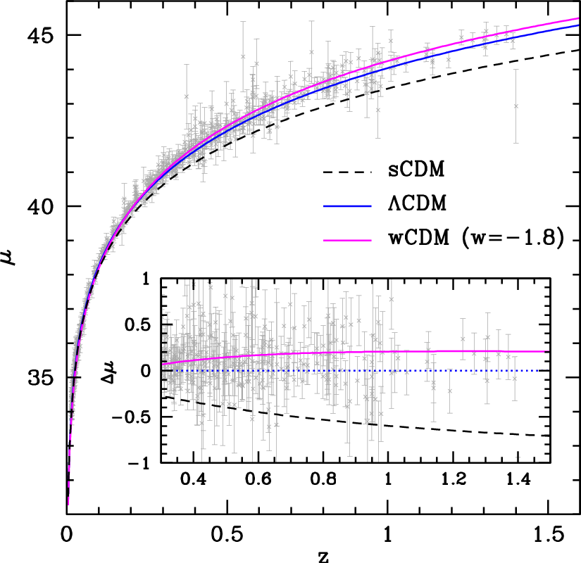
Let us also outline that results are marginally different if SNIa data replace data; SNIa and data, however, are not independent and should not be simultaneously used. In Figure 4 we however show the distance modulus , obtained for CDM and other cosmologies, against observational distance moduli provided by the Union2 Supernova Cosmology Project [7]. The upper solid (magenta) curve, in the main frame, is obtained for . ’s are also plotted, in respect to a CDM model. There can be scarce doubts that a model with is in perfect agreement with SNIa data.
4 Phantom and neutrinos
There is a wide literature on models with , following the original proposal by [16] of an anomalous kinetic energy for the DE scalar field. The main physical context where such phantom DE was advocated where the limits on neutrino () masses (see, e.g., [17]).
Let then be the sum of the -mass eigenvalues, for ’s belonging to the usual three particle families. The point we wish to make here is that, if we force to shift to values smaller than those obtainable by freely best fitting cosmological data, so to approach constraints, we simultaneously obtain two results: (i) decreasing DE state parameters are met; (ii) upper limits on are gradually softened. This is shown in Figure 5.
The (i) point is consistent with the results of the previous Section. The only difference being that the dataset considered here includes SNIa, instead of data.

As far as the (ii) point is considered, we show the effects of taking two specific values. The former one is the value corresponding to the fit at , discussed in the previous Section. The slight discrepancy from the range found here arises from two reasons: (i) data are replaced by SNIa data. (ii) Different parameters are set free: here is fixed and (the fraction of Dark Matter due to ’s) is free, the opposite choice with respect to Figure 3.
The meaning of the Figure is however clear: If data are approached, -mass constraint soften. If we opt for the closer model allowing some agreement with , the upper limit on shifts from 1.12 eV to 1.27 eV. If we go as down as is needed to meet the g.a. line, we find a limit at 1.56 eV. Furthermore, in the latter case, there is an apparent 1.7 ’s “detection” for . Such pseudo-detection would take a completely different significance if particle data would yield a neutrino mass detection in a similar mass range.
5 Discussion
It may be worth outlining soon that phantom DE is not a straightforward result of quantum field theory. If DE is a scalar field, its energy density and pressure arise from the kinetic and potential energy densities ( and , respectively) according to the relations
| (3) |
so that approaches when , but is unable to bypass the limit unless lays in the interval .

Another option is that data analysis tends to favor because Cold Dark Matter (CDM) and DE are coupled and the assumed parameter space does not include a coupling parameter. In other terms: measuring could be the consequence of assuming no energy flow from CDM to DE if they are actually coupled.
In this case, data can be approached by using an effective DE energy density [19]
| (4) |
being the CDM-DE coupling (see, e.g., [20]). The state parameter of DE reads then
| (5) |
with
| (6) |
provided that is constant. It must be however outlined that this is however an approximate treatment, yielding increasingly rougher results as the coupling increases. In Figure 6 we give an example of the redshift dependence of , for a RP model [21] with cosmological parameters close to WMAP7 best fit (, , , and shown in the frame). In this straightforward case, we find a variable effective state parameter which, averaged on between and , yields As a matter of fact, however, models yielding significantly more negative averages are hard to build, unless assuming that itself suitably depends on The point is that, when increasing , there arise apparent instabilities in , even below On the contrary, coupled DE models with similar ’s, independently of their capacity to meet data, certainly exhibit no such instabilities. Henceforth, the capacity to mimic CDM-DE coupling by means of an effective potential is limited.
However, if is suggested by data, this can be generically interpreted as possibly favoring CDM-DE coupling.
In recent work, the option of CDM-DE coupling has been specifically tested against data, by simultaneously allowing for higher [22, 23], finding that such Mildly Mixed Coupled (MMC) models exhibit a likelihood slightly exceeding CDM (below the 2- level). We plan to reconsider such option in the presence of priors towards lower .
6 Conclusions
The main task of this note is testing the consequence of taking data on the same foot of other light nuclide abundances. BBN constraints, when is disregarded, yield no real parameter limitation in top of those arising from CMB, BAO, SNIa, , etc. : the BBN interval set by , , and , sometimes set as a prior, more or less overlaps with WMAP interval for CDM cosmologies.
On the contrary, if is considered, BBN is a real extra constraint to cosmological models and DE state equations with are favored together with values smaller by -, in respect to the interval usually considered.
Within this context, limits are softened up to 1.6 eV, but the really new feature is a quasi-detection for a non-vanishing eV.
A more general, very tentative, conclusion is that there is a realistic possibility that WMAP data, for some still unknown reason, led to slightly overestimate ; if such estimate is reduced by 4-5, then, a different cosmological scenario seems to open: a simple CDM cosmology is no longer so close to data, predictions of light element abundances by BBN would approach a general self-consistency, an energy flow from CDM to DE could mimic a unique nature of the dark components, and eV could turn into an actual detection.
Acknowledgements.
The authors wish to thank F. Matteucci for Figure 1 and for insightful discussions. This work was partially supported by ASI (the Italian Space Agency) thanks to the contract I/016/07/0 ”COFIS”. S.B. acknowledges the support of the Italian Center for Space Physics (CIFS) through the C.I. no. 2010/24 .References
- (1) F. Matteucci, Proc. IAU Symp. 268 (2010) 453
- (2) F. Iocco, G. Mangano, G. Miele, O. Pisanti and P. D. Serpico, Phys. Rept. 472 (2009) 1
- (3) E. Komatsu et al. [WMAP Collaboration], Astrophys. J. Suppl. 192 (2011) 18
- (4) A. Lewis and S. Bridle, Phys. Rev. D 66 (2002) 103511
- (5) B. A. Reid et al. [SDSS Collaboration], Mon. Not. Roy. Astron. Soc. 401 (2010) 2148
- (6) A. G. Riess et al., Astrophys. J. 699 (2009) 539
- (7) R. Amanullah et al., Astrophys. J. 716 (2010) 712
- (8) F. Spite and M. Spite, Astron. and Astrophys. 115 (1982) 357
- (9) D. L. Lambert and B. E. Reddy, Mon. Not. Roy. Astron. Soc. 349 (2004) 757
- (10) C. Charbonnel and F. Primas, Astron. and Astrophys. 442 (2005) 961
- (11) M. Asplund, D. L. Lambert, P. E. Nissen, F. Primas and V. V. Smith, Astrophys. J. 644 (2006) 229
- (12) P. Bonifacio, L. Pasquini, P. Molaro, E. Carretta, P. François, R. G. Gratton, G. James, L. Sbordone, F. Spite and M. Zoccali, Astron. and Astrophys. 470 (2007) 153
- (13) L. Sbordone, M. Limongi, A. Chieffi, E. Caffau, H. G. Ludwig and P. Bonifacio, Astron. and Astrophys. 503 (2009) 121
- (14) W. Aoki et al., AIP Conf. Proc. 847 (2006) 53
- (15) D. Romano, F. Matteucci, P. Ventura and F. D’Antona, Astronomy and Astrophysics 374 (2001) 646; Romano et al. (2011), in prep.
- (16) R. R. Caldwell, Phys. Lett. B 545 (2002) 23
- (17) K. Ichikawa and T. Takahashi, Phys. Rev. D 73 (2006) 083526
- (18) E. Komatsu et al. [WMAP Collaboration], Astrophys. J. Suppl. 180 (2009) 330
- (19) S. Das, P. S. Corasaniti and J. Khoury, Phys. Rev. D 73 (2006) 083509
- (20) L. Amendola, Phys. Rev. D 62 (2000) 043511
- (21) B. Ratra and P. J. E. Peebles, Phys. Rev. D 37 (1988) 3406
- (22) G. La Vacca, J. R. Kristiansen, L. P. L. Colombo, R. Mainini and S. A. Bonometto, JCAP 0904 (2009) 007;
- (23) J. R. Kristiansen, G. La Vacca, L. P. L. Colombo, R. Mainini and S. A. Bonometto, New Astron. 15 (2010) 609