The Physics of the Neutrino Mechanism of Core-Collapse Supernovae

The velocity structure of spherical steady-state isothermal flows is described by the equation

where $\mathscr{M}=v/c_{T}$ is the Mach number, $v$ is the fluid velocity, $c_{T}$ is the isothermal sound speed, $x=rc_{T}^{2}/(2GM)$ is the rescaled radial coordinate $r$, and $M$ is the mass of the central object. It is possible for a standing shock wave in the flow to exist at a point that satisfies the two Rankine-Hugoniot shock jump conditions

which express conservation of mass and momentum, respectively. Here, $\rho$ is the mass density and the $+$ and $-$ superscripts correspond to the quantities evaluated just upstream and downstream of the shock, respectively. The physically relevant solution to equations (2–3) is $\mathscr{M}^{+}\mathscr{M}^{-}=1$.

In Figure 1, we show with black solid lines Mach-number profiles of flows with a single constant mass accretion rate $\dot{M}=-1\,M_{\odot}\ {\rm s}^{-1}$ obtained by solving equation (1). The integration starts at a fixed radius $r_{\nu}$ corresponding to the surface of the star, and with a fixed velocity $v_{\nu}=\dot{M}/(4\pi r_{\nu}^{2}\rho_{\nu})$, where $\rho_{\nu}$ is the prescribed mass density at $r_{\nu}$. Different lines correspond to different values of $c_{T}^{2}$. The dashed line shows the decelerating transonic solution, which goes through the sonic point²² 2 In this paper we assign the name “sonic point” to the position of the flow where the numerator and denominator of the fluid momentum equation simultaneously vanish. Although this point is generally called the “critical point”, we avoid this name to prevent confusion with the critical neutrino luminosity discussed later in the paper. located at $x_{\rm sonic}=0.25$ and $\mathscr{M}_{\rm sonic}=-1$. It has high velocity at large radii and $\mathscr{M}\rightarrow 0$ as $x\rightarrow 0$, unlike Bondi accretion flow, which starts with zero velocity at infinity, goes through the sonic point and has $\mathscr{M}\rightarrow-\infty$ as $x\rightarrow 0$ (shown with dash-dotted line). The decelerating transonic solution separates accretion “breezes”, which are always subsonic ($-1<\mathscr{M}\leq 0$) and denoted as B, from solutions going through $\mathscr{M}=-1$ and denoted as A. Although the A-type solutions lying below the decelerating transonic solution are considered unphysical in standard Bondi accretion theory, the parts of these solutions that span from $r_{\nu}$ to the shock are viable in this setting [43].

The dotted lines in Figure 1 show the velocities just downstream of the shock, $\mathscr{M}^{-}$, corresponding to three different assumed profiles of the upstream velocities $\mathscr{M}^{+}$: (1) Bondi flow (blue), (2) free fall with $\mathscr{M}^{+}=-x^{-1/2}$ (green), and (3) pressure-less free fall (red), that is a good approximation in more realistic supernova calculations [15] and that requires modification of equation (3) by assuming that $\mathscr{M}^{+}=-x^{-1/2}\ll-1$, and

The physically relevant solution to equations (2) and (a) is $\mathscr{M}^{-}=(\sqrt{x^{-1}-4}-x^{-1/2})/2$. For the sake of clarity, we do not show the upstream profiles in Figure 1 except for Bondi flow (dash-dotted line).

The velocity profile of the shocked accretion flow for a given $c_{T}$ is constructed by following one of the black lines from $r_{\nu}$ until it crosses a dotted line that corresponds to the appropriate shock jump conditions. At this intersection, the solution jumps to whatever velocity profile $\mathscr{M}^{+}$ was assumed to be present upstream.

The essential point of Figure 1 is that for a fixed $\dot{M}$ the presence of a shock is not guaranteed for all values of $c_{T}$. For example, consider the blue dotted line, which corresponds to Bondi accretion flow upstream of the shock. For the smallest values of $c_{T}$, the required shock radius — the intersection of the black solid line with blue dotted line — would be below the radius of the star, an unphysical situation. As we step to higher $c_{T}$, the shock appears at $r_{\nu}$ and moves outward. At a critical value $c_{T}^{\rm crit}$ corresponding to the decelerating transonic accretion flow (dashed line), the shock can only coincide with the sonic point at $x^{\rm crit}=x_{\rm sonic}=0.25$. Here there is no jump in the velocity, and the shock degenerates into a jump in the derivative of the velocity [59, 16]. A shock is not possible for $c_{T}>c_{T}^{\rm crit}$, because the blue dotted line lies below the decelerating transonic solution (dashed line) in the range of radii of interest and hence B-type solutions are not viable solutions inside the shock – that is, solutions of type B do not intersect the blue dotted line.

The situation is somewhat different when the flow upstream of the shock is in free fall, as shown with the red and green dotted lines in Figure 1. In these cases, the shock jump conditions allow part of the B-type solutions as viable solutions downstream of the shock. Furthermore, for values of $c_{T}$ higher than that corresponding to the decelerating transonic solution (dashed line) two shock radii are possible for a single value of $c_{T}$, because the curvature of B-type solutions and shock jump conditions yields two intersections. When stepping to higher values of $c_{T}$, the two shock radii come closer together and finally coincide at a critical value $c_{T}^{\rm crit}$. Contrary to the case of Bondi flow above the shock, there is no relation between the critical sound speed $c_{T}^{\rm crit}$ and the sonic point. The shock radius at $c_{T}^{\rm crit}$ also does not coincide with the velocity minimum of any of the B-type solutions. Above the critical sound speed $c_{T}^{\rm crit}$, a shock in the flow is not possible, qualitatively similar to the case of Bondi flow (blue dotted line) described above.

Finally, we briefly discuss the “upper” solutions that appear when $c_{T}$ is higher than the value corresponding to the decelerating transonic solution (dashed line in Fig. 1), but still $c_{T}<c_{T}^{\rm crit}$. We see that the maximum shock radius for these solutions is identical to the sonic point radius. The shock radius decreases with increasing $c_{T}$ until it merges with the normal solution branch at $c_{T}^{\rm crit}$. These upper solutions were found by Yamasaki & Yamada [64] also in the full problem, but these authors show that the upper solutions are unstable to perturbations and thus most likely do not occur in a real physical system. Because of this, we do not discuss the upper solutions further except in Sections III.2 and III.3.

In Figure 2 we show the critical values $c_{T}^{\rm crit}$ as a function of mass accretion rate $\dot{M}$ for the three sets of shock jump conditions shown in Figure 1. The three curves are similar over a significant range of $\dot{M}$ despite the relatively stark differences in the shock jump conditions. Specifically, the top and the middle curves closely resemble the bottom blue line, which is, in fact, the relation between the sound speed and the mass-accretion rate for isothermal transonic accretion [35, p. 68]. The curvature of this relation in the log-log plane of Figure 2 arises from exponential near-hydrostatic density profile of the atmosphere, which is a good approximation to the decelerating transonic accretion flow below the sonic point.

From Figure 1 it is obvious that for pressure-less free fall upstream of the shock the solution described by $c_{T}^{\rm crit}$ does not correspond to any special radial point in the flow. However, we also see that the shock position $x^{\rm crit}$ at $c_{T}^{\rm crit}$ is constant when expressed in the dimensionless coordinates since this is the point where the dotted line just meets the flow profile. Changes in $\dot{M}$, $\rho_{\nu}$ or $r_{\nu}$ only move the starting inner point of the flow, but one can always find a value of $c_{T}=c_{T}^{\rm crit}(\dot{M},\rho_{\nu},r_{\nu})$ to get the critical solution at $x^{\rm crit}$. By plugging the solution of $\mathscr{M}^{-}$ from the shock jump condition in equation (a) into equation (1)³³ 3 We note that this procedure is valid only for determining the position of the critical point in isothermal accretion. As seen from Figure 1, the critical point occurs when the line of all possible shock positions (solution to eqs. [2] and [a], dotted red line) just touches the flow profiles (solutions to eq. [1], solid black lines). Thus, at this point only, the tangents and values are the same, which we then use to calculate the position of the critical point, equation (4)., we obtain exactly $x^{\rm crit}=3/16$ implying that the critical condition for existence of steady-state accretion shock in isothermal accretion is

where $v_{\rm esc}=\sqrt{2GM/r}$ is the escape velocity. This result is valid when the flow upstream of the shock is in free fall and has negligible thermal pressure. We note that equation (4) is valid only at $c_{T}^{\rm crit}$. There are indeed shock solutions with $x_{\rm shock}>x^{\rm crit}$ that correspond to the upper solution branch as discussed in Sections II.1 and III.2 and by Yamasaki & Yamada [64], but these solutions still have $c_{T}<c_{T}^{\rm crit}$. The actual value of $c_{T}^{\rm crit}$ for given $\dot{M}$, $M$, $r_{\nu}$, and $\rho_{\nu}$ is calculated numerically as is demonstrated in Figure 2.

As the ratio in equation (4) is lower than for the sonic point, we call this condition “antesonic” (see footnote 1). For the case of free fall with non-negligible pressure shown with green line in Figure 1, the numerical factor is $(5-\sqrt{21})/2\simeq 0.2087$. Furthermore, we emphasize that equation (4) does not imply any connection to the Parker point⁴⁴ 4 The Parker point occurs when the right-hand side of equation (1) vanishes, and in the case of isothermal flow the Parker point coincides with the sonic point [35, p. 63]. or sonic point. Thus, one cannot assume that the existence of a shock is equivalent to the existence of a sonic point in the context of supernova stalled accretion shocks [52, as in]. However, if the flow upstream of the shock is a Bondi accretion flow with the same sound speed, then the critical condition is exactly the same as the expression for the position of the sonic point: $(c_{T}^{\rm crit}/v_{\rm esc})^{2}=0.25$.

Our calculation of the critical condition in equation (4) also explains why the critical curves for different shock jump conditions in Figure 2 are so similar: their values can be estimated in the same way as for the position of the sonic point [35, p. 68], except that for the shock jump conditions relevant in the supernova context the value of $x^{\rm crit}$ is lower than $0.25$ (eq. [4]).

For the sake of completeness, we repeated the isothermal calculation with pressure-less free fall above the shock for a polytropic equation of state $P=k\rho^{\Gamma}$, where $k$ is the normalization factor and $\Gamma$ is the adiabatic index, which we vary from $1$ to $1.7$. We do not assume energy conservation through the shock so that $k$ is left as a free parameter, which we can vary to obtain its critical values. The results are qualitatively similar to those for isothermal accretion. For fixed $\Gamma$, there exists a critical value of the constant $k$ above which there are no steady-state solutions with a bounding shock. As in the isothermal case, this critical value of $k$ corresponds to a critical condition that can be written as $\max\,(c_{S}^{2}/v_{\rm esc}^{2})\approx 0.19\Gamma$ (compare with eq. [4]), where $c_{S}$ is the adiabatic sound speed and the “antesonic factor” is linearly proportional to the adiabatic index of the flow. We illustrate the dependence of $\max\,(c_{S}^{2}/v_{\rm esc}^{2})$ on $\Gamma$ in Figure 3. where we plot the antesonic ratio as a function of $k$ for a range of $\dot{M}$ and two values of $\Gamma$. We note that although we are able to write down a single local criterion for the antesonic condition in the adiabatic case, at the radial location where $\max\,(c_{S}^{2}/v_{\rm esc}^{2})$ occurs, this condition should be interpreted as a global condition on the flow, and not a local one. As in the isothermal case, the physics of the critical condition is determined by the ability of the flow to satisfy the jump conditions while simultaneously satisfying the Euler equations for steady-state accretion.

The physics of collapse, core bounce and shock stall dictate that there is a phase of steady-state accretion flow with a standing shock with time-changing $\dot{M}$ and $c_{T}$. If $c_{T}$ slowly increases at fixed $\dot{M}$, the shock radius advances until the critical value $c_{T}^{\rm crit}$ is reached. Physically, $c_{T}^{\rm crit}$ exists because as $c_{T}$ is increased the shock jump conditions simply cannot be satisfied given the properties of the flow upstream and the necessity of maintaining conservation of mass and momentum. What happens at $c_{T}^{\rm crit}$ depends on the properties of the flow upstream of the shock. In the case of Bondi flow, the profile can continuously transition to a shock-less B-type solution (accretion breeze) as shown by Korevaar [34], Velli [59], Velli [60] and Del Zanna et al. [16], because there is no jump in velocity at $c_{T}^{\rm crit}$. However, in the case relevant for supernovae, where the flow above the shock is in pressure-less free fall, the shock does not degenerate at $c_{T}^{\rm crit}$ and a catastrophic dynamical transition must occur, most likely to a supersonic wind, which can be identified with the supernova explosion [10, 11, 12]. A similar conclusion was reached by Yamasaki & Yamada [64]. It is likely that time-dependent hydrodynamical instabilities will modify the exact realization of this scenario. Nevertheless, our results from the isothermal accretion model are an important step towards understanding the mechanism of supernova explosions, and specifically the neutrino mechanism, as we detail below. Our isothermal model also provides a robust explosion criterion of broad applicability (the “antesonic” condition, Section IV.4).

We solve the time-independent Euler equations

where $P$ is the gas pressure, $M$ is the mass within the radius of the neutrinosphere $r_{\nu}$, $\varepsilon$ is the internal specific energy of the gas, and $\dot{q}=\mathcal{H}-\mathcal{C}$ is the net heating rate, a difference of heating $\mathcal{H}$ and cooling $\mathcal{C}$. These hydrodynamic equations couple through the equation of state (EOS), $P(\rho,T,Y_{\rm e})$ and $\varepsilon(\rho,T,Y_{\rm e})$, where $T$ is the gas temperature, to the equation for electron fraction $Y_{\rm e}$

where $l_{\nu_{\rm e}n}$, $l_{e^{+}n}$, $l_{{\overline{\nu}_{\rm e}}p}$, and $l_{e^{-}p}$ are reaction rates involving neutrons and protons. In Appendix A we provide equations (5–7) in the form of separated radial derivatives, which is useful for describing the connection between the critical luminosity and $c_{T}^{\rm crit}$ of Section II. We also employ, for the first time in the context of calculations of the critical luminosity, gray neutrino radiation transport using the expression

where $L_{\nu}$ is the combined luminosity of electron neutrinos and antineutrinos, which are assumed to be equal everywhere. We do not consider neutrinos of other flavors. We assume that neutrinos have root-mean-square energy of $\epsilon_{\nu_{e}}=13$ MeV and antineutrinos $\epsilon_{\bar{\nu}_{e}}=15.5$ MeV [57]. Even this very simple approximation to radiation transport enables us to assess the relative importance of accretion and core neutrino luminosity for the supernova explosion. Our choice of equation of state, heating and cooling function, and reaction rates is a simplified version of Scheck et al. [50] and Qian & Woosley [49]. More details are given in Appendix A.

Five equations (5–9) are solved on an interval of radii between $r_{\nu}$ and $r_{\rm S}$, where $r_{\nu}$ is the radius of the neutrinosphere and is fixed, and $r_{\rm S}$ is the radius of the shock, which is left to vary. The matter inside of $r_{\nu}$ is the PNS core and is characterized only by its mass $M$ and luminosity $L_{\nu,\,{\rm core}}$ and energy of neutrinos and antineutrinos that it isotropically emits.

We thus need six boundary conditions to uniquely determine five functions: $\rho$, $v$, $T$, $Y_{\rm e}$ and $L_{\nu}$, and shock radius $r_{\rm S}$. We first demand that the flow has a fixed mass accretion rate $\dot{M}=4\pi r^{2}\rho v$ by applying this constraint at the inner boundary. We assume that the neutrino luminosity at the inner boundary is equal to the luminosity of the PNS core, $L_{\nu}(r_{\nu})=L_{\nu,\,{\rm core}}$. At the outer boundary we apply the shock jump conditions⁵⁵ 5 We do not include nuclear binding energy in our calculations. However, the pertinent effects are qualitatively assessed in Appendix A and in Yamasaki & Yamada [65].

where $v_{\rm ff}=\sqrt{\Upsilon}v_{\rm esc}$ is the free fall velocity, and in accordance with analytically estimated accretion data of Woosley et al. [63] supernova progenitor models available on-line⁶⁶ 6 http://www.stellarevolution.org/data.shtml we choose $\Upsilon=0.25$. The quantity $\rho^{+}$ is the density just upstream of the shock and can be calculated from conservation of mass. We also assume that the matter entering the shock is composed of iron and hence $Y_{\rm e}=26/56$ at the outer boundary. The last boundary condition comes from requirement that $r_{\nu}$ is the neutrinosphere for electron neutrinos, which gives a constraint on the optical depth

where $\kappa_{\nu_{e}}$ is the opacity to electron neutrinos. This condition is implemented by adding an extra variable corresponding to the optical depth and requiring that it is zero at the inner boundary and $2/3$ at the outer boundary.

The equations and boundary conditions above are solved using a relaxation algorithm [47, p. 753] with logarithmic spacing of grid points [see 56, and references therein]. The number of grid points was usually $\gtrsim 1000$. We refer to the problem outlined by equations (5–12) and the physics described in Appendix A as the “fiducial calculation”. As this problem is complex, we occasionally resort to various simplifications to make some of our points more clear. We describe what exactly we modified with respect to the fiducial calculation at a various places in the text.

We include neutrino radiation transport and hence our solutions are parameterized by the core neutrino luminosity $L_{\nu,\,{\rm core}}$ and yield neutrino luminosity as a function of radius $L_{\nu}(r)$. We confirm the existence of an upper limit to the core neutrino luminosity $L_{\nu,\,{\rm core}}^{\rm crit}$ at fixed $\dot{M}$ [11, 64, 65]. We determine $L_{\nu,\,{\rm core}}^{\rm crit}$ by starting the relaxation code at a low value of $L_{\nu,\,{\rm core}}$ with an initial guess of power-law profiles of variables, and then increase $L_{\nu,\,{\rm core}}$ in small steps while using the converged solution from the previous step as an initial guess for the next step. We use bisection to trace $L_{\nu,\,{\rm core}}^{\rm crit}$ to a specified relative precision.

Figure 4 shows profiles of thermodynamic quantities for $L_{\nu,\,{\rm core}}$ stepping from $0$ to $L_{\nu,\,{\rm core}}^{\rm crit}$. Similar plots except for $L_{\nu}(r)$ were published previously by Yamasaki & Yamada [64], Yamasaki & Yamada [65], but we reproduce them here for the sake of completeness. Our results fall within the paradigm of quasi-steady-state supernova structure [6, 39, 29, e.g.]. In particular, we find a steep decrease in the density outside $r_{\nu}$ that flattens when the dominant pressure support changes from an ideal gas of nucleons to a relativistic gas of electrons and positrons. The temperature profile is flat at small $r$, but then drops as the relativistic particles become more dominant. Still, the temperature changes only from approximately $3$ MeV to $0.5$ MeV, much less than the corresponding change by several orders of magnitude in density. This implies that our isothermal model is a legitimate rough approximation of the problem. We discuss in more detail the profiles of the adiabatic sound speed $c_{S}$, total specific energy in the form of Bernoulli integral⁷⁷ 7 The importance of individual terms contributing to $\mathscr{B}$ is assessed in Appendix B.

and neutrino luminosity $L_{\nu}$ that are to our knowledge not previously discussed in the context of the calculation of $L_{\nu,\,{\rm core}}^{\rm crit}$.

The total specific energy $\mathscr{B}$ is an increasing function of $L_{\nu,\,{\rm core}}$ in the whole region of interest. The maximum of $\mathscr{B}$ occurs at $r_{\rm gain}$, which is defined as $\dot{q}(r_{\rm gain})=0$. Both $r_{\rm gain}$ and $\mathscr{B}(r_{\rm gain})$ increase with increasing $L_{\nu,\,{\rm core}}$. We note that even at $L_{\nu,\,{\rm core}}^{\rm crit}$ the energy is significantly negative in the entire region of interest. It is certainly not the case that positive $\mathscr{B}$ corresponds to explosion [12, $L_{\nu,\,{\rm core}}=L_{\nu,\,{\rm core}}^{\rm crit}$;].

The adiabatic sound speed $c_{S}$ was calculated using equation (A9) and is plotted in the bottom left of Figure 4 as a ratio to the local escape velocity $v_{\rm esc}(r)$. Similar to $\mathscr{B}$, we see that an increase of $L_{\nu,\,{\rm core}}$ results in a net increase of $c_{S}$ between $r_{\nu}$ and $r_{\rm S}$. The maximum of $c_{S}$ occurs at gradually larger radii for increasing $L_{\nu,\,{\rm core}}$, similar to the gain radius $r_{\rm gain}$. However, the maximum of $c_{S}^{2}/v_{\rm esc}^{2}$ does not exactly coincide with $r_{\rm gain}$; in fact, $r_{\rm gain}$ is always about $1$ to $2\%$ larger for the particular calculation shown in Figure 4.

The middle center panel of Figure 4 shows profiles of $L_{\nu}(r)$. As expected, $L_{\nu}$ grows in the cooling layer as a result of net neutrino and antineutrino production and decreases in the gain layer as a result of heating. How much does the accreting material cooling via neutrino emission contribute to the total neutrino flux emanating from below the shock? We define the accretion neutrino luminosity $L_{\nu}^{\rm acc}$ as the difference between the neutrino luminosity at the shock and the luminosity of the core,

The relative contribution of the accretion luminosity to the total neutrino luminosity decreases with growing $L_{\nu,\,{\rm core}}$. For $L_{\nu,\,{\rm core}}=0$, the accretion luminosity is the sole contributor to the total luminosity of about $1.4\times 10^{52}$ ergs s^-1, but for the critical core luminosity of $6.41\times 10^{52}$ ergs s^-1 the accretion luminosity contributes $28\%$ to the total neutrino output. Clearly, the accretion luminosity is a sub-dominant, but important part of the total neutrino output. In Section III.4 we investigate how including the neutrino radiation transport and hence accretion luminosity affects $L_{\nu,\,{\rm core}}^{\rm crit}$ for a range of $\dot{M}$.

We now turn our attention to another aspect of steady-state accretion shocks: the existence of two solutions with different shock radii for some values of $L_{\nu,\,{\rm core}}$, discovered by Yamasaki & Yamada [64]. These authors also performed linear stability analysis and found that the upper solution branch with higher $r_{\rm S}$ is unstable, the lower branch is stable, and both branches meet at a marginally stable point at $L_{\nu,\,{\rm core}}^{\rm crit}$. We confirm the presence of the upper solution branch with our code. We switch to the upper solution branch by first calculating a sequence of models on the lower branch up to $L_{\nu,\,{\rm core}}^{\rm crit}$. We take a solution close to $L_{\nu,\,{\rm core}}^{\rm crit}$, manually scale up the radial coordinates by about $50\%$ and let the relaxation algorithm converge to a solution on the upper branch.

We find that the profiles of thermodynamic variables for the upper solution branch are not fundamentally different from those of the lower branch presented in Figure 4 and hence we do not present them here. We plot in Figure 5 the shock radii and total specific energies at several radii of interest for both branches, and as a function of $L_{\nu,\,{\rm core}}$ for several values of $\dot{M}$. We see that the upper branch of solutions extends to larger shock radii, but ends at a finite radius and non-zero $L_{\nu,\,{\rm core}}$ (left panel, Figure 5). We specifically checked that this is not an artifact in our calculation. We note however, that for different input physics the upper branch can end at much larger radii, consistent with infinity in our code. We also find that the specific energy of the upper solution is always higher than that of the lower solution for the same $L_{\nu,\,{\rm core}}$ at all radii. In analogy with other physical systems that have two states with different energy, we can argue that the higher energy upper solution branch is unstable to transition, in agreement with Yamasaki & Yamada [64] who find that the upper branch is indeed unstable to radial perturbations. We do not discuss the properties of the upper branch in greater detail, because it is unlikely that these solutions would be realized in a real physical system. However, the existence of the upper solution branch is analoguous to the upper solutions in Figure 1.

It has been clearly established in 1D calculations that there exists an upper limit to the core neutrino luminosity $L_{\nu,\,{\rm core}}^{\rm crit}$ that allows for a steady-state accretion shock [11, 64, 65], and this limit has been confirmed to exist in multi-dimensional dynamical supernova simulations [44, 45], and in simulations of the stalled accretion shock [46, 27]. To illustrate how the upper limit on the core neutrino luminosity is related to the limit on the sound speed in isothermal accretion discussed in Section II, we consider the total specific energy of the system $\mathscr{B}$, which has the property that its radial derivative is proportional to the net deposited heating and cooling:

It is well established [29, e.g.] and we confirm this in Appendix B, that the contribution of the kinetic term $v^{2}/2$ to the total specific energy budget in equation (13) is negligible. At a fixed radius $r$ in the gain layer where $\dot{q}\approx L_{\nu,\,{\rm core}}/r^{2}$, the increase of $L_{\nu,\,{\rm core}}$ will result in an increase of enthalpy $h=\varepsilon+P/\rho$, and consequently, of the adiabatic sound speed, as $h\sim c_{S}^{2}$. We showed in Section III.2 that $c_{S}$ as well as $\mathscr{B}$ at a given radius are increasing functions of $L_{\nu,\,{\rm core}}$ everywhere, not only in the gain layer. This correspondence between $L_{\nu,\,{\rm core}}$ and $c_{S}$ suggests that $L_{\nu,\,{\rm core}}^{\rm crit}$ is a realization of $c_{T}^{\rm crit}$ (Section II) in the context of the neutrino heating mechanism.

As shown in Section II, $c_{T}^{\rm crit}$ occurs when the flow cannot satisfy the shock jump conditions at any point in the accretion flow [64, see also]. We now prove that the same mechanism is responsible for the existence of $L_{\nu,\,{\rm core}}^{\rm crit}$ in the supernova context. Essentially, we are trying to construct an equivalent of Figure 1 for non-isothermal flows and more realistic physics. In order to make this feasible we consider a simplification of the problem by setting ${\rm d}Y_{\rm e}/{\rm d}r=0$ and ${\rm d}L_{\nu}/{\rm d}r=0$ (eqs. [8] and [9]) and setting the heating and cooling terms to $\mathcal{H}=1.2\times 10^{-18}\,{\rm cm^{2}\ g^{-1}}L_{\nu,\,{\rm core}}/r^{2}$ and $\mathcal{C}=2\times 10^{18}\,(T/{\rm MeV})^{6}$ ergs s^-1 g^-1, respectively. We also modify the boundary conditions by requiring $\rho(r_{\nu})=3\times 10^{10}$ g cm^-3 instead of fixing $\tau_{\nu}$. With these changes, the problem simplifies considerably, because $\rho(r_{\nu})$ and $v(r_{\nu})$ are now fixed and the only variables left are $T(r_{\nu})$ and $r_{\rm S}$, which are determined by the two shock jump conditions. Consequently, if we know the value of $T(r_{\nu})$, the flow profile is now uniquely determined as an initial value problem.

We want to show how the solution for the flow structure with a shock relates to all possible accretion solutions. For a given $L_{\nu,\,{\rm core}}$ and $T(r_{\nu})$ we calculate the A-type solutions (those reaching $\mathscr{M}=-1$ in Figure 1) by setting $v^{2}=c_{S}^{2}$ at the outer boundary, which gives a continuum of solutions for a range of $T(r_{\nu})$. Solutions going through the sonic point are obtained by setting the numerator and denominator of the momentum equation (A2) simultaneously to zero at the outer boundary. The accretion breezes (B-type solutions in Figure 1) are obtained from the A-type solutions by setting $v$ to a specific fraction of $c_{S}$ at a fixed radius corresponding to $v=c_{S}$ in an A-type solution. By varying this fraction, we get a continuum of flows with different $T(r_{\nu})$. We extend the breezes to larger radii with an initial-value integrator of stiff equations based on algorithms from Press et al. [47] and using the results from our relaxation algorithm as a starting point. We verified that for B-type solutions (subsonic accretion breezes) the ratio $|v/c_{S}|$ is always less than unity.

In the left panel of Figure 6 we show the position of the shock radius $r_{\rm S}$ (solid) and the sonic point $r_{\rm sonic}$ (dashed) as a function $L_{\nu,\,{\rm core}}$. In the right panel, we show the values of $T(r_{\nu})$ for the same solutions as in the left panel. We see that $r_{\rm sonic}$ exhibits qualitatively similar behavior to $r_{\rm S}$, except that for low values of $L_{\nu,\,{\rm core}}$ there is no sonic point with a finite $r_{\rm sonic}$. Furthermore, the position of the shock is well separated from the sonic point, except for the tip of the upper solution branch, where these two appear to merge, similar to what happens in isothermal accretion in Figure 1. The same trend is seen in $T(r_{\nu})$ (the only free parameter of the problem for fixed $L_{\nu,\,{\rm core}}$), which suggests that the upper branches of shock and sonic point indeed coincide at some $L_{\nu,\,{\rm core}}$.

In order to explore the situation in more detail, we selected four values of $L_{\nu,\,{\rm core}}$ marked by vertical dot-dashed lines to illustrate the four configurations visible in Figure 6: (1) low $L_{\nu,\,{\rm core}}$ with one solution with finite shock radius and no finite sonic radius, (2) intermediate $L_{\nu,\,{\rm core}}$ where two solutions are present for both the shock and the sonic point, (3) $L_{\nu,\,{\rm core}}>L_{\nu,\,{\rm core}}^{\rm crit}$ but with two sonic point solutions still present, and (4) high $L_{\nu,\,{\rm core}}$ with no solution for either the shock or the sonic point. In Figure 7 we plot flow solutions for each of these luminosities (black solid lines) with shock jump conditions overplotted (green solid lines). The Figure should be interpreted in a way similar to Figure 1. We found that plotting the Mach number of the flows only obfuscates the issue because the lines cross in a complicated manner; instead we plot momentum $\rho v^{2}+P$ and specific energy $\mathscr{B}$. In this parameter space the different flow lines generally do not intersect and the shock jump conditions are a function of only the radius as can be seen from the equations (10) and (11).

The upper left part of Figure 7 shows flow profiles for low $L_{\nu,\,{\rm core}}$, where there is only one solution for the shock radius (far left vertical dash-dotted line in Figure 6). Each solid line corresponds to a different value of $T(r_{\nu})$. For low $T(r_{\nu})$, we find that the flows are of type A. That is, they reach a point where $v^{2}=c_{S}^{2}$ (not a sonic point; shown with black dots in Figure 7). For increasing $T(r_{\nu})$, the intersection of the flow with the shock jump conditions moves to larger radii. A-type solutions extend to $T(r_{\nu})\simeq 3.32$ MeV, where the point where $v^{2}=c_{S}^{2}$ moves to infinite radius. For yet larger $T(r_{\nu})$ we are able to find only B-type solutions — subsonic accretion breezes — with $|v/c_{S}|<1$ everywhere. For a single value of $T(r_{\nu})$ the profiles of momentum and energy of the flow intersect with the shock jump conditions at the same radius, which means that only at this $T(r_{\nu})$ is a solution with a shock possible (red line). The vertical dotted lines mark radii of intersection of momentum of the flow with the momentum shock jump condition. We then plot these radii in the energy panel and we see that for flows lying below the red line the intersection of $\mathscr{B}$ with the appropriate shock jump condition occurs at systematically smaller radii than what is required by the momentum profiles. Conversely, for curves above the red line the intersection occurs at larger radii. Thus, the momentum and energy at the shock can only be conserved simultaneously for a single $T(r_{\nu})$ at $L_{\nu,\,{\rm core}}=5\times 10^{51}$ ergs s^-1, which then defines not only $T(r_{\nu})$, but also $r_{\rm S}$.

The upper right panel of Figure 7 displays flow profiles for intermediate $L_{\nu,\,{\rm core}}$, which allows for two solutions for the shock and the sonic point (vertical dash-dotted line labelled (2) in Figure 6). The topology of the solutions for this $L_{\nu,\,{\rm core}}$ differs from the previous case. The A-type solutions exist only for a small range of temperatures ($3.517\,{\rm MeV}<T(r_{\nu})<3.675\,{\rm MeV}$). There are two transonic solutions going through two distinct sonic points at finite but vastly different radii, which separate A-type solutions from the B-type solutions, (which occur for $T(r_{\nu})<3.517$ MeV and $T(r_{\nu})>3.675$ MeV). Due to severe stiffness of the equations, we were not able to follow the B-type solutions to very large radii. In contrast to the upper left panel of Figure 7 at lower $L_{\nu,\,{\rm core}}$, the flow profiles intersect the shock jump conditions at just two inner boundary temperatures shown by the two solid red lines. The upper solutions are analoguous to those obtained in the isothermal model in Figure 1.

The lower left part of Figure 7 explores the region with $L_{\nu,\,{\rm core}}>L_{\nu,\,{\rm core}}^{\rm crit}$ where two solutions for the sonic point are still present. The topology of the solutions is similar to the previously discussed case with $L_{\nu,\,{\rm core}}=5\times 10^{52}$ ergs s^-1, except that the A-type solutions exist for an even smaller range of inner boundary temperatures ($3.852\,{\rm MeV}<T(r_{\nu})<3.875$ MeV). However, in this case, there are no simultaneous intersections of the momentum and energy profiles of the flows with the shock jump conditions. This is explicitly shown by the vertical dotted lines, which mark several radii of intersection of the momentum profiles of the flows with the momentum shock jump condition. Clearly, the intersections of the energy profiles with the energy shock jump conditions occur at systematically smaller radii. This means that at this $L_{\nu,\,{\rm core}}$ no flow profile can connect to the free-falling matter upstream, because it is not possible to simultaneously satisfy conservation of mass, momentum and energy at the shock. Although the mismatch in radii decreases as we go to the higher $T(r_{\nu})$ of B-type solutions, they eventually cease to cross the energy shock jump condition altogether. Overall, as implied by Figure 6, for $L_{\nu,\,{\rm core}}=9.5\times 10^{52}$ ergs s^-1 it is impossible to find a flow solution that simultaneously conserves momentum and energy at the shock.

For the sake of completeness we show in the lower right panel of Figure 7 the flow profiles for high $L_{\nu,\,{\rm core}}$, where there is no possible solution with a shock or a sonic point. All flows displayed are B-type solutions with $|v/c_{S}|<1$. Despite the fact that we were not able to extend some of the solutions to large radii due to stiffness of the equations, $v/c_{S}$ of the solutions systematically converged to zero at large radii.

With the $L_{\nu,\,{\rm core}}$–$T(r_{\nu})$ space systematically explored we can now label regions of A and B solutions in Figure 6 in analogy with Figure 1. We note that the more physically realistic simulation displayed in Figure 5 has exactly the same behavior except that sonic points exist at finite radii all the way to $L_{\nu,\,{\rm core}}=0$. The upper shock solution branch, however, ends as indicated in Figure 5. As can be seen from Figure 6, the position of the shock when $L_{\nu,\,{\rm core}}=L_{\nu,\,{\rm core}}^{\rm crit}$ does not align with the position of the sonic point and hence a smooth transition to a B-type solution is not possible, unlike the results of Korevaar [34], Velli [59], Velli [60] and Del Zanna et al. [16]. With the same logic as in Section II we argue that at $L_{\nu,\,{\rm core}}^{\rm crit}$ the structure of the accretion flow catastrophically changes: if $L_{\nu,\,{\rm core}}>L_{\nu,\,{\rm core}}^{\rm crit}$ the shock moves outwards dynamically and a neutrino-driven wind with a sonic point below the shock is established. However, multi-dimensional time-dependent hydrodynamical instabilities might modify the realization of this process.

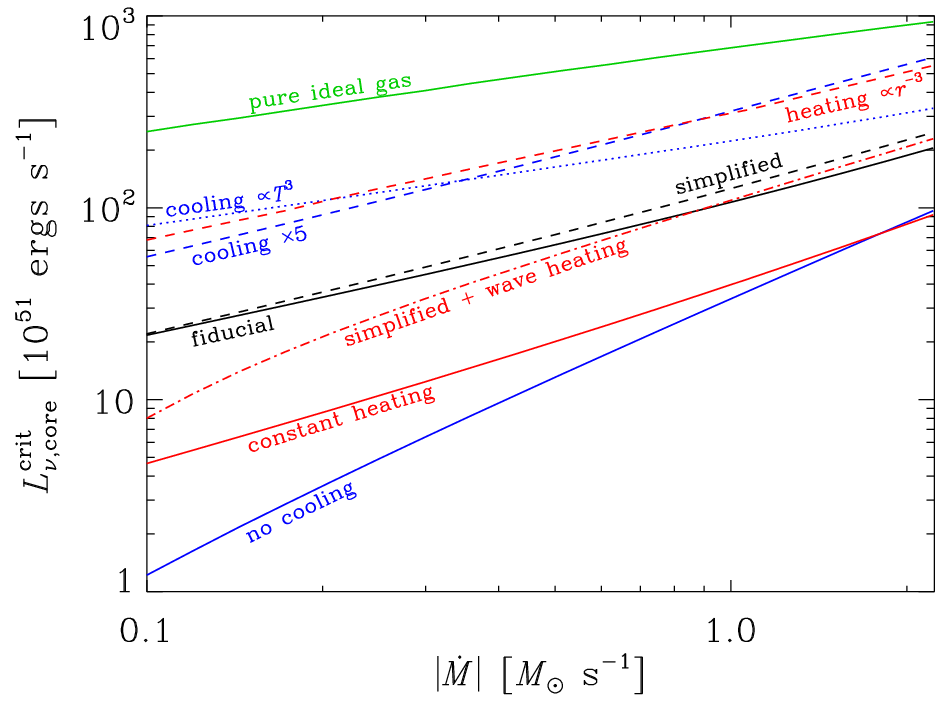
In Figure 8 we present the critical core neutrino luminosity $L_{\nu,\,{\rm core}}^{\rm crit}$ versus the mass accretion rate, the critical curve, as calculated with the fiducial physical model as described in Section III.1. Before we dive into properties of the critical curve, we investigate whether it is a robust phenomenon from the point of view of input physics. To this end, we simplify the problem by setting the electron chemical potential to zero, shutting off neutrino radiation transport (${\rm d}L_{\nu}/{\rm d}r=0$), electron fraction evolution (${\rm d}Y_{\rm e}/{\rm d}r=0$), and choosing simplified heating and cooling prescription with $\mathcal{H}_{\rm s}=1.2\times 10^{-18}L_{\nu,\,{\rm core}}/r^{2}$ and $\mathcal{C}_{\rm s}=8.19\times 10^{-43}\,T^{6}$, respectively. The critical curve for this modification is shown in Figure 8 with a dashed black line. With respect to the simplified version of the calculation we make additional individual changes to see how the critical curve changes: we modify cooling by multiplying it by a factor of $5$, making it proportional to $T^{3}$ instead of $T^{6}$, or shutting it off altogether. We modified heating by making it proportional to $r^{-3}$, constant at all radii or adding to $\mathcal{H}_{\rm s}$ heating motivated by Alfvén wave energy deposition [40]. We also changed the EOS to be that of a pure ideal gas. We also tried an EOS of pure relativistic particles, but we were able to converge to solution only by relaxing the condition on optical depth and replacing it with fixed density at $r_{\nu}$. We thus do not show the critical curve here.

Figure 8 shows that even drastic changes to the functional form of the heating and cooling functions and EOS consistently yield critical values of $L_{\nu,\,{\rm core}}$. Naturally, the exact value of $L_{\nu,\,{\rm core}}^{\rm crit}$ at a given $\dot{M}$ changes considerably. However, it is interesting that we do not see wildly discrepant slopes of individual lines in Figure 8. Specifically, changing the form of the heating affects the slope only very slightly, while the form of cooling has a much more pronounced effect, except when simply multiplied by a constant factor. This can be explained by the fact that cooling couples directly to the temperature, and the temperature gradient is directly responsible for the hydrostatic equilibrium of the region when relativistic gas dominates.

In order to obtain dependencies of $L_{\nu,\,{\rm core}}^{\rm crit}$ on the parameters for the fiducial problem (solid line in Figure 8), we determine critical core luminosities on a grid of parameter values chosen as $M\in\{1.2,1.4,1.6,1.8,2.0\}\,M_{\odot}$, $r_{\nu}\in\{20,40,60\}$ km, $\tau_{\nu}\in\{1/6,1/3,2/3\}$, and 30 values of $\dot{M}$ logarithmically spaced between $-0.01\,M_{\odot}\ {\rm s^{-1}}$ and $-2\ M_{\odot}\ {\rm s^{-1}}$. Although in principle the neutrinosphere radius $r_{\nu}$ and core luminosity $L_{\nu,\,{\rm core}}$ are connected by physics of neutrino diffusion out of the PNS, we consider them separately here. The critical curves for sample values of parameters are shown in the left panel of Figure 9. In addition to the well-known dependence of $L_{\nu,\,{\rm core}}^{\rm crit}$ on $\dot{M}$, we see that $L_{\nu,\,{\rm core}}^{\rm crit}$ increases with increasing $M$ and decreasing $r_{\nu}$ and $\tau_{\nu}$. Lower values of $\tau_{\nu}$ also increase the curvature of the lines in the $\dot{M}$–$L_{\nu,\,{\rm core}}^{\rm crit}$ space. In order to quantify these observations we fit to all our results a combination of power laws to get

The relative differences between calculated and fitted values of $L_{\nu,\,{\rm core}}^{\rm crit}$ are plotted in the right panel of Figure 9. On the first sight, the multiple power-law fit of equation (16) is not perfect. However, for most of the data the power-law fit is good within $30\%$ of $L_{\nu,\,{\rm core}}^{\rm crit}$. There are systematic trends in the residuals as a function of $\dot{M}$ in the sense that all lines are curved upward: at low and high $\dot{M}$ the value of $L_{\nu,\,{\rm core}}^{\rm crit}$ is slightly higher than what would correspond to the mean power law fitted to the data. We can understand this on the basis of our isothermal accretion model and its critical curve presented in Figure 2, which also exhibits an upward curvature of the critical curves, which is a manifestation of the nearly-hydrostatic exponential density structure of the flow (see Section II).

In the fit of equation (16) we did not include the dependence on the remaining parameters of our calculation, including the incoming electron fraction $Y_{\rm e}(r_{\rm S})$, and energy of the neutrinos $\epsilon_{\nu_{e}}$ and antineutrinos $\epsilon_{\bar{\nu}_{e}}$. We performed a simple check to see how changes in these parameters affect $L_{\nu,\,{\rm core}}^{\rm crit}$. We find that changing $Y_{\rm e}(r_{\rm S})$ from $0.45$ to $0.5$ shifts the critical luminosity by at most $1\%$. As suggested by the physics of the neutrino heating, $L_{\nu,\,{\rm core}}^{\rm crit}$ scales as $\epsilon_{\nu_{e}}^{-2}$. We confirm this scaling to within $2\%$ by varying $\epsilon_{\nu_{e}}$ from $8$ MeV to $14$ MeV while keeping the ratio $\epsilon_{\nu_{e}}/\epsilon_{\bar{\nu}_{e}}$ fixed at $13/15.5\simeq 0.839$.

One of the uncertainties in core-collapse supernova simulations and neutron star physics in general is the EOS of dense matter. For example, a softer high-density nuclear EOS generically leads to smaller PNS radii at earlier times after collapse and bounce, but also leads to higher average neutrino energies, which might be favorable for explosion [1, 2, 53, 30, 38, e.g.]. Can we put some constraints on the EOS using our results on $L_{\nu,\,{\rm core}}^{\rm crit}$? In more realistic simulations, $L_{\nu,\,{\rm core}}$, $r_{\nu}$ and the temperature of emitted neutrinos $T_{\nu}\sim\epsilon_{\nu_{e}}$ are connected by the physics of diffusion. In the simplest case, we can assume that these quantities follow the black-body law

where $\sigma$ is the Stefan-Boltzmann constant. In addition to equation (16) we found that $L_{\nu,\,{\rm core}}^{\rm crit}\sim\epsilon_{\nu_{e}}^{-2}$ to a very good precision. Eliminating the dependence on $\epsilon_{\nu_{e}}$ using equation (17), we find

Therefore, larger neutrinosphere radii suggest lower $L_{\nu,\,{\rm core}}^{\rm crit}$, when all other quantities are equal. Thus, stiff equations of state that yield higher $r_{\nu}$ are potentially preferred. We note that this result is enabled by superlinear dependence of $L_{\nu,\,{\rm core}}^{\rm crit}$ on $r_{\nu}$ in equation (16). On the other hand, soft EOS leads to a faster contraction of the PNS, higher core luminosities and neutrino energies, which can be favorable for the explosion too [50, 51, 37, 38].

Finally, we briefly mention the behavior of shock radii at $L_{\nu,\,{\rm core}}^{\rm crit}$, $r_{\rm S}^{\rm crit}$. In Figure 10, we plot $r_{\rm S}^{\rm crit}/r_{\nu}$ as a function of $L_{\nu,\,{\rm core}}^{\rm crit}$ for data from Figure 9. We see that the points lie close to a line described approximately as $r_{\rm S}^{\rm crit}/r_{\nu}\propto({L_{\nu,\,{\rm core}}^{\rm crit}})^{-0.26}$. The weak dependence on $L_{\nu,\,{\rm core}}^{\rm crit}$ can probably be attributed to changes in the efficiency of cooling as a function $L_{\nu,\,{\rm core}}^{\rm crit}$ and hence $\dot{M}$ (see Section V.3 for a related discussion). There are no noticeable residuals as a function of $r_{\nu}$, $M$, and $\tau_{\nu}$.

As we have demonstrated in Section III.4, the critical luminosity depends on $\dot{M}$, $M$ and $r_{\nu}$. A natural combination of these variables to have the dimension of luminosity is $GM\dot{M}/r_{\nu}$, an expression for power released by accretion of material. Although the powers of individual quantities are somewhat different than those in equation (16), one might wonder whether these expressions for the critical luminosity are intimately related in the sense that $L_{\nu,\,{\rm core}}^{\rm crit}$ is directly proportional to $L_{\nu}^{\rm acc}$. This interpretation is especially tempting, because dynamical supernova models seem to be on the verge of explosion over a wide range of $\dot{M}$, which would suggest that a significant fraction of the neutrino luminosity is supplied by cooling of the accreting gas. Any change in $\dot{M}$ yields a proportional change of $L_{\nu}^{\rm acc}$, which again somehow proportionally changes the critical luminosity while keeping it higher than $L_{\nu}^{\rm acc}$. This picture is, however, incorrect.

To illustrate why, we plot in Figure 11 $L_{\nu,\,{\rm core}}^{\rm crit}$ along with the neutrino luminosity leaving the shock $L_{\nu}(r_{\rm S})$ at $L_{\nu,\,{\rm core}}^{\rm crit}$, and their difference, $L_{\nu}^{\rm acc}$. We also plot $GM\dot{M}/r_{\nu}$, corresponding to the maximum achievable $L_{\nu}^{\rm acc}$ for a cold accretion flow. We see that $L_{\nu}^{\rm acc}$ is always a small fraction of $L_{\nu,\,{\rm core}}^{\rm crit}$, and that even the maximum possible value of $L_{\nu}^{\rm acc}$ falls short of the necessary luminosity by a factor of several as found also by Burrows & Goshy [11]. Clearly, the major source of neutrinos powering the explosion is the core of the PNS. However, the accretion luminosity is not entirely unimportant. We plot in Figure 11 $L_{\nu,\,{\rm core}}^{\rm crit}$ for a calculation with the same parameters but with neutrino radiation transport shut off. Including the radiation transport in the calculation has a positive effect of lowering the critical core luminosity by about $8\%$ at $\dot{M}=-0.01\,M_{\odot}$ s^-1 and by about $23\%$ at $\dot{M}=-2\,M_{\odot}$ s^-1, respectively.

Instead of regarding equation (16) as a manifestation of accretion luminosity, we can understand it in the terms of the critical condition on the sound speed in isothermal accretion given in equation (4). The dependencies of equation (16) can be then explained in simple terms. Increasing the mass of the PNS core makes the escape velocity higher and velocity profile steeper, and more heating is then necessary to get a mild enough velocity profile that it can no longer connect to the shock jump conditions (Section II). Increasing $r_{\nu}$ shifts the region of interest to weaker gravitational potential with lower escape velocity and hence lower neutrino luminosity is required to get a mild velocity profile that again does not connect to the shock jump conditions. Decreasing $\tau_{\nu}$ with all other parameters fixed means less neutrinos absorbed and clearly a higher critical neutrino luminosity is required.

To illustrate this in greater detail, we can write $\dot{q}/v\sim{\rm d}c_{S}^{2}/{\rm d}r\sim c_{S}^{2}/r_{\nu}$ and hence $c_{S}^{2}\sim h\sim\dot{q}r_{\nu}/v\sim\rho_{\nu}r_{\nu}L_{\nu,\,{\rm core}}/\dot{M}$, where $h$ is the enthalpy and $\rho_{\nu}$ is the density at the neutrinosphere. Plugging this expression as $c_{T}^{\rm crit}$ in equation (4), we obtain $L_{\nu,\,{\rm core}}^{\rm crit}\sim GM\dot{M}/(\rho_{\nu}r_{\nu}^{2})$. The product $\rho_{\nu}r_{\nu}$ is proportional to the optical depth $\tau_{\nu}$, because most of opacity to the neutrinos is concentrated close to the neutrinosphere. Thus, by relating $c_{T}^{\rm crit}$ of the isothermal accretion model through Euler equations to $L_{\nu,\,{\rm core}}^{\rm crit}$ we arrive through a simple estimate to essentially the same expression for $L_{\nu,\,{\rm core}}^{\rm crit}$ as in the dimensional analysis in the beginning of this Section. The power-law dependence of these estimates is of course different than in the empirical fit in equation (16) due to nonlinear nature of the problem.

Several authors have produced critical curves based on either steady-state calculations like our own, or hydrodynamic simulations. Through steady-state calculations, Burrows & Goshy [11] obtained a critical curve that is best fit by a power law, $L_{\nu,\,{\rm core}}^{\rm crit}\sim\dot{M}^{0.43}$. This power-law slope is lower by about $0.3$ than what we measure. This difference can be reconciled by realizing that Burrows & Goshy [11] assumed that the neutrinosphere radius $r_{\nu}$ is determined by $L_{\nu,\,{\rm core}}$ and neutrino temperature $T_{\nu}$ through a black-body law. If we substitute equation (17) to equation (16) to eliminate $r_{\nu}$, we get

The power-law slope in $\dot{M}$ is about $0.40$, quite close to Burrows & Goshy [11].

In Figure 12 we compare our results to the critical curves of Nordhaus et al. [45] based on hydrodynamic simulations. In order to make our calculations compatible with theirs, we couple $r_{\nu}$ to $L_{\nu,\,{\rm core}}$ through equation (17) with $T_{\nu}=4.5$ MeV. We keep $M$ fixed at $1.4\,M_{\odot}$, which makes the slope of our critical curves slightly milder than that of Nordhaus et al. [45]: for a given progenitor model lower, but fixed, $L_{\nu,\,{\rm core}}$ means that the explosion occurred later when $M$ is higher, because the PNS had a longer time to gain mass, and hence $L_{\nu,\,{\rm core}}^{\rm crit}$ is higher. We see that our results are in good agreement with Nordhaus et al. [45] and that including heating from accretion luminosity reduces $L_{\nu,\,{\rm core}}^{\rm crit}$ by an amount comparable to going from 1D to 2D or from 2D to 3D.

Bethe & Wilson [3] were the first to analyze the delayed neutrino mechanism. They argued that shock recession creates a steeper pressure profile that in turn overcomes gravitation and gives an outward acceleration, $\ddot{r}>0$. In the language of our steady-state model, $\ddot{r}=v({\rm d}v/{\rm d}r)>0$ is the statement of their critical explosion condition. From Figure 4 we clearly see that below the shock the flow decelerates everywhere, except maybe for a small range of radii, where $v$ is basically constant. We also find through an investigation of the velocity profiles that having ${\rm d}v/{\rm d}r=0$ somewhere in the flow does not correlate with approaching the critical curve at different $\dot{M}$. In the discussion of our toy model in Section V and in Appendix B we show that velocity and acceleration terms are subdominant in the momentum and energy equation of the problem and that $L_{\nu,\,{\rm core}}^{\rm crit}$ does not depend on these terms. From this evidence we conclude that the vanishing acceleration criterion of Bethe & Wilson [3] does not coincide with the critical neutrino luminosity.

Janka [29] presented a quasi-time-dependent analytic analysis of the conditions necessary for revival of a stalled accretion shock. He found that the shock experiences both expansion and outward acceleration when both the mass and energy in the gain region grow with time. These conditions define two critical lines in the $L_{\nu,\,{\rm core}}$–$\dot{M}$ plane that enclose a region favorable for explosion. As the approach of Janka [29] is completely different from that of Burrows & Goshy [11] and also ours, his critical condition is also very different. As can be seen in Figures 4 and 5 of Janka [29], the critical luminosities are decreasing function of increasing $|\dot{M}|$, unlike the plots in Burrows & Goshy [11], Yamasaki & Yamada [64], Yamasaki & Yamada [65], and our Figure 11, where the critical luminosities increase with increasing $|\dot{M}|$.

In Figure 13, we plot as a function of $L_{\nu,\,{\rm core}}$ and $\dot{M}$ the mass in the gain layer, $M_{\rm gain}=\int_{r_{\rm gain}}^{r_{\rm S}}4\pi r^{2}\rho\,{\rm d}r$, total mass between the neutrinosphere and the shock, $M_{\rm tot}$, energy in the gain layer, $E_{\rm gain}=\int_{r_{\rm gain}}^{r_{\rm S}}4\pi r^{2}\rho(\varepsilon-GM/r)\,{\rm d}r$, and the total energy between the neutrinosphere and the shock $E_{\rm tot}$. We see that for a model with fixed mass accretion rate the masses grow with increasing $L_{\nu,\,{\rm core}}$ as $L_{\nu,\,{\rm core}}^{\rm crit}$ is approached. While the total energy at any specific radius in the gain layer increases with growing $L_{\nu,\,{\rm core}}$ (see Figure 4 for a plot of the related Bernoulli integral), the total energy within that region decreases, because the gain layer gets physically larger with increasing $L_{\nu,\,{\rm core}}$.

The critical conditions of Janka [29] demand that the mass and energy in the gain region increase with time. As there is no time dependence in our steady-state models and thus this condition is not directly testable, we might emulate the time dependence with a sequence of steady-state models. If we fix $\dot{M}$ and increase $L_{\nu,\,{\rm core}}$, following either of the lines in Figure 13, $M_{\rm gain}$ grows and $E_{\rm gain}$ decreases. On the other hand, if we fix $L_{\nu,\,{\rm core}}$ to, say, $5\times 10^{51}$ ergs s^-1 and decrease $|\dot{M}|$, which corresponds to moving vertically from red through blue to black lines in Figure 13, $M_{\rm gain}$ first drops and then increases. Similarly, $E_{\rm gain}$ first increases and then just before reaching the critical curve it decreases. Thus, from the point of view of our steady-state models, the conditions of Janka [29] are not equivalent to the critical neutrino luminosity.

The ratio of advection to heating time $t_{\rm adv}/t_{\rm heat}$ has been extensively used as a metric of hydrodynamic simulations [54, 55, 58, 9, 51, e.g.]. Murphy & Burrows [44] found that this condition is only a rough diagnostic of the critical condition for explosion.

Here, we specifically test two definitions of advection and heating times. The first is an integral condition on the gain layer due to Murphy & Burrows [44]

We plot in Figure 14 values of the ratio $t^{\prime}_{\rm adv}/t^{\prime}_{\rm heat}$ for a range of mass accretion rates. To a factor of $\sim\!2$ the condition $t^{\prime}_{\rm adv}/t^{\prime}_{\rm heat}\sim 1$ at $L_{\nu,\,{\rm core}}^{\rm crit}$. However, the specific value of the ratio changes from about $0.7$ to almost $1.2$ over the range of mass accretion rates – more than a $50\%$ increase. Clearly, this definition does not exactly correspond to the critical luminosity.

The second definition of advection and heating times is due to Thompson et al. [58], who defined the times locally as

where $r_{P}=({\rm d}\ln P/{\rm d}r)^{-1}$ is the pressure scale-height at a given radius. In Figure 15 we plot the ratio $t^{\prime\prime}_{\rm adv}/t^{\prime\prime}_{\rm heat}$ as a function of radius for two values $\dot{M}$. For the smaller $\dot{M}$, the ratio spikes to high values below the gain radius, while it stays consistently below unity above it, even though the critical luminosity was reached. Contrary to this, the higher $\dot{M}$ calculation tolerates $t^{\prime\prime}_{\rm adv}/t^{\prime\prime}_{\rm heat}>1$ in the gain layer for a number of sub-critical luminosities.

Neither definition of advection and heating times yields the desired exact correspondence with $L_{\nu,\,{\rm core}}^{\rm crit}$. We tried to adjust the definitions in many ways, but failed to produce a condition that would be valid over a wide range of parameters (e.g., $\dot{M}$, $M$, and $r_{\nu}$).

In Section II we showed that the antesonic condition $(c_{T}^{\rm crit})^{2}/v_{\rm esc}^{2}=0.1875$ is equivalent to the critical condition for isothermal accretion with pressure-less free fall at the shock, and it can be generalized to $\max\,(c_{S}^{2}/v_{\rm esc}^{2})\approx 0.19\Gamma$ for a polytropic EOS. Does a similar condition hold also in the more realistic calculations? In order to test this, we studied the maximum value of the ratio of the adiabatic sound speed $c_{S}$ to the escape velocity, $\max\,(c_{S}^{2}/v_{\rm esc}^{2})$, similarly to the polytropic case. We plot in Figure 16 how this value changes with core luminosity and mass accretion rate. We find that the value of this parameter is surprisingly constant at $\max\,(c_{S}^{2}/v_{\rm esc}^{2})\approx 0.20$ over almost three orders of magnitude in $\dot{M}$ at $L_{\nu,\,{\rm core}}=L_{\nu,\,{\rm core}}^{\rm crit}$. Furthermore, we took all $1350$ critical luminosities used to construct Figure 9 and calculated a histogram of values of $\max\,(c_{S}^{2}/v_{\rm esc}^{2})$ at $L_{\nu,\,{\rm core}}^{\rm crit}$. We find that the histogram can be very well fit with a Gaussian with a maximum at $0.193$ and with a width of $0.009$, that is only $5\%$ of its value! While from Figure 16 we observe in critical values a slight trend with $\dot{M}$, we also see from the same Figure that the numerical noise contributes significantly to the total scatter⁸⁸ 8 Although critical luminosities can be determined very precisely with our code, other parameters like critical shock radii are determined less precisely. This is because $|\partial r_{\rm S}/\partial L_{\nu,\,{\rm core}}|=\infty$ at the critical luminosity, as can be inferred from Figure 5. Hence, a small uncertainty in $L_{\nu,\,{\rm core}}^{\rm crit}$ is dramatically amplified in $r_{\rm S}$ and related quantities, as can be noted in Figures 14 and 16..

How does the value of $\max\,(c_{S}^{2}/v_{\rm esc}^{2})$ depend on input physics? We determined $\max\,(c_{S}^{2}/v_{\rm esc}^{2})$ for data of Figure 8 and found that there is some variability. For constant heating (solid red line) the ratio is about $0.15$, while for no cooling (solid blue line) and heating proportional to $r^{-3}$ (red dashed line) the mean value is about $0.26$. For all other cases of different physics, the mean value ranges from $0.19$ to $0.22$, quite close to the result from our fiducial calculation. Furthermore, we also find that increasing $\Upsilon$, the fraction of free-fall velocity of the incoming matter (eq. [11]), from $0.25$ to unity increases the value of the ratio from $0.19$ to about $0.22$. We found in Section II that for polytropic EOS the antesonic ratio is linearly proportional to adiabatic index $\Gamma$. With this information at hand, the close agreement between $\max\,(c_{S}^{2}/v_{\rm esc}^{2})$ measured in our fiducial calculation and the value in isothermal accretion can be regarded as a coincidence. The fiducial calculation is not exactly isothermal ($\Gamma>1$), which compensates for lowering $\Upsilon$ to $0.25$. Even so, despite the fact that $L_{\nu,\,{\rm core}}^{\rm crit}(\dot{M})$ changes dramatically with the large changes to the input physics considered in Figure 8, $\max\,(c_{S}^{2}/v_{\rm esc}^{2})$ is virtually constant $\sim\!0.2$.

Another question is how does the radius at which $c_{S}^{2}/v_{\rm esc}^{2}$ peaks relate to other significant radii of the problem like the gain and shock radii? In the isothermal calculation this critical radius coincides with the shock radius, because at this position the escape velocity is smallest. In the full problem this is clearly not the case as shown in the lower left panel of Figure 4. Instead we find that radius of maximum $c_{S}^{2}/v_{\rm esc}^{2}$ nearly coincides with the gain radius, but that they are offset by as much as $2\%$ in both directions. For the case of no cooling, the maximum occurs at the neutrinosphere, and there is no gain radius. As the radius of maximum $c_{S}^{2}/v_{\rm esc}^{2}$ closely tracks the gain radius in the fiducial calculation, their difference might not be noticeable at all in simulations.

Burrows et al. [12] proposed a similar “coronal” condition for the explosion, where $T$ of the substantial amount of matter needs to be higher than the local escape temperature. However, we have demonstrated that the transition from accretion to wind does not require sound speeds above the escape speeds. Instead, the sound speed vs. escape speed condition is only a manifestation of the inability to satisfy the shock jump conditions. Indeed, as Figure 4 shows, the Bernoulli integral is negative at explosion as noted also by Burrows et al. [12].

Our toy model is based on the assumption of hydrostatic equilibrium, conservation of energy, and the fact that $L_{\nu,\,{\rm core}}^{\rm crit}$ occurs when the shock jump conditions cannot be simultaneously matched to any solution of the Euler equations (Section II). We find that we can realistically model $L_{\nu,\,{\rm core}}^{\rm crit}$ using the solution to simple algebraic equations. Specifically, we obtain a quadratic equation for $r_{\rm S}$, which gives $L_{\nu,\,{\rm core}}^{\rm crit}$ when the discriminant vanishes. The cost of this simplicity is that we must introduce a number of approximations, albeit reasonable, and are forced to make our model somewhat internally inconsistent. Therefore, our toy model produces only qualitative agreement with the numerical solution. Even this approach, however, enables us to grasp the basic elements of the physics involved and to extend them to more complicated and more complete models (see Appendix B).

A primary simplification of the model is that we take the heating and cooling functions to depend only on radius $r$: $\mathcal{H}(r)=aL_{\nu,\,{\rm core}}/r^{2}$ and $\mathcal{C}(r)=b/r^{4}$. While $\mathcal{H}$ is a good approximation, $\mathcal{C}$ lacks the important self-regulatory feature of realistic cooling, which is proportional to $T^{6}$, that an excess in the internal energy can be quickly radiated away. In other words, when no heating is present, the material cannot radiate away via neutrino cooling more energy than its total internal energy content. To quantify this constraint on the cooling function $\mathcal{C}(r)$, we assume that a cold parcel of matter falls from large distance through the shock to the neutrinosphere at $r_{\nu}$. When no heating is present, the parcel will radiate a fraction of its gravitational potential energy

where $\eta$ is the cooling efficiency. If the sole source of neutrino flux is the accretion flow itself (ie. there is no $L_{\nu,\,{\rm core}}$), then $\eta\leq 1$. In the presence of heating we still consider equation (22) to be valid, but with a different (and potentially higher) value of $\eta$. A condition similar to equation (22) was employed by Fernández & Thompson [18] to limit excessive cooling due to discreteness effects.

Shock radii as a function of $L_{\nu,\,{\rm core}}$ and $L_{\nu,\,{\rm core}}^{\rm crit}$ as a function of $\dot{M}$ are shown in Figures 17 and 18, respectively, at two levels of approximation. In both, the results from the numerical solution to equations (B1) and (B2) are labelled “numerical” and the results from a truly analytic toy model are labelled “toy.” We find that equations (B7) and (B8) from the toy model, which provide explicit analytic solutions for $r_{\rm S}$ and $L_{\nu,\,{\rm core}}^{\rm crit}$, reproduce the qualitative behavior of the more complete solution remarkably well.

Is it possible to reach $L_{\nu,\,{\rm core}}^{\rm crit}$ with just $L_{\nu}^{\rm acc}$? Within the framework of the toy model, the answer to the question of whether $L_{\nu,\,{\rm core}}^{\rm crit}$ is always higher than $\eta GM|\dot{M}|/r_{\nu}$ depends on the ratio of the term in the square brackets in equation (B10) (which is always positive and larger than unity) to the denominator, $2\pi r_{\nu}\rho_{\nu}a$, an upper limit of the optical depth $\tau_{\nu}$ for our fixed density profile. For small $\eta$ we can thus write (see eq. B8)

where the exact factor in front of the right-hand side is comparable to, but always higher than unity. For parameters given in Table 1 we get $\tau_{\nu}\approx 2\pi r_{\nu}\rho_{\nu}a\doteq 0.36$ and $L_{\nu,\,{\rm core}}^{\rm crit}>\eta GM|\dot{M}|/r_{\nu}$. We confirmed this result for all $0<\eta\leq 1$ by inspecting graphs similar to Figure 18.

From equation (23) we see that if $\tau_{\nu}\sim 1$, then even if the whole region between the neutrinosphere and the accretion shock is immersed in a neutrino flux corresponding to the maximum integrated neutrino cooling $\eta GM\dot{M}/r_{\nu}$, the critical luminosity cannot be attained. Furthermore, if $\eta\gtrsim\tau_{\nu}$ then the critical luminosity is even higher than the maximum gravitational energy release rate. In reality, the accretion luminosity available for absorption will be substantially lower than in the ideal scenario described, and hence sufficient core neutrino luminosity independent of the accretion flow is required to reach an explosion. One could rightfully argue that the optical depth is not constrained within our toy model and that at high $\tau_{\nu}$ some effect might come to play that lowers the critical luminosity below the accretion luminosity. However, as demonstrated by our numerical solution to the more detailed version of the problem described in Section III.4 and depicted in Figure 11, $L_{\nu,\,{\rm core}}^{\rm crit}$ is in fact much higher than the maximum possible accretion luminosity.

References

- [1] Baron, E., Cooperstein, J., & Kahana, S. 1985, Physical Review Letters, 55, 126
- [2] Baron, E., Cooperstein, J., & Kahana, S. 1985, Nuclear Physics A, 440, 744
- [3] Bethe, H. A., & Wilson, J. R. 1985, ApJ, 295, 14
- [4] Blondin, J. M., Mezzacappa, A., & DeMarino, C. 2003, ApJ, 584, 971
- [5] Blondin, J. M., & Mezzacappa, A. 2006, ApJ, 642, 401
- [6] Bruenn, S. W. 1985, ApJS, 58, 771
- [7] Bruenn, S. W., De Nisco, K. R., & Mezzacappa, A. 2001, ApJ, 560, 326
- [8] Buras, R., Rampp, M., Janka, H.-T., & Kifonidis, K. 2006a, A&A, 447, 1049
- [9] Buras, R., Janka, H.-T., Rampp, M., & Kifonidis, K. 2006b, A&A, 457, 281
- [10] Burrows, A. 1987, ApJ, 318, L57
- [11] Burrows, A., & Goshy, J. 1993, ApJ, 416, L75
- [12] Burrows, A., Hayes, J., & Fryxell, B. A. 1995, ApJ, 450, 830
- [13] Burrows, A., Livne, E., Dessart, L., Ott, C. D., & Murphy, J. 2006, ApJ, 640, 878
- [14] Burrows, A., Livne, E., Dessart, L., Ott, C. D., & Murphy, J. 2007, ApJ, 655, 416
- [15] Colgate, S. A., & White, R. H. 1966, ApJ, 143, 626
- [16] Del Zanna, L., Velli, M., & Londrillo, P. 1998, A&A, 330, L13
- [17] Dessart, L., Burrows, A., Livne, E., & Ott, C. D. 2006, ApJ, 645, 534
- [18] Fernández, R., & Thompson, C. 2009, ApJ, 697, 1827
- [19] Fernández, R. 2010, ApJ, 725, 1563
- [20] Foglizzo, T. 2002, A&A, 392, 353
- [21] Fryer, C. L., & Heger, A. 2000, ApJ, 541, 1033
- [22] Fryer, C. L., & Warren, M. S. 2002, ApJ, 574, L65
- [23] Fryer, C. L., & Warren, M. S. 2004, ApJ, 601, 391
- [24] Hanke, F., Marek, A., Mueller, B., & Janka, H.-T. 2011, arXiv:1108.4355
- [25] Herant, M., Benz, W., & Colgate, S. 1992, ApJ, 395, 642
- [26] Herant, M., Benz, W., Hix, W. R., Fryer, C. L., & Colgate, S. A. 1994, ApJ, 435, 339
- [27] Iwakami, W., Kotake, K., Ohnishi, N., Yamada, S., & Sawada, K. 2008, ApJ, 678, 1207
- [28] Janka, H.-T., & Müller, E. 1996, A&A, 306, 167
- [29] Janka, H.-T. 2001, A&A, 368, 527
- [30] Janka, H.-T., Buras, R., Kitaura Joyanes, F. S., Marek, A., Rampp, M., & Scheck, L. 2005, Nuclear Physics A, 758, 19
- [31] Janka, H.-T., Müller, B., Kitaura, F. S., & Buras, R. 2008, A&A, 485, 199
- [32] Keil, W., Janka, H.-T., & Mueller, E. 1996, ApJ, 473, L111
- [33] Kitaura, F. S., Janka, H.-T., & Hillebrandt, W. 2006, A&A, 450, 345
- [34] Korevaar, P. 1989, A&A, 226, 209
- [35] Lamers, H. J. G. L. M., & Cassinelli, J. P. 1999, Introduction to Stellar Winds, pp. 452. Cambridge, UK: Cambridge University Press, June 1999.
- [36] Liebendörfer, M., Mezzacappa, A., Thielemann, F.-K., Messer, O. E., Hix, W. R., & Bruenn, S. W. 2001, Phys. Rev. D, 63, 103004
- [37] Marek, A., & Janka, H.-T. 2009, ApJ, 694, 664
- [38] Marek, A., Janka, H.-T., Müller, E. 2009, A&A, 496, 475
- [39] Mayle, R., & Wilson, J. R. 1988, ApJ, 334, 909
- [40] Metzger, B. D., Thompson, T. A., & Quataert, E. 2007, ApJ, 659, 561
- [41] Mezzacappa, A., Calder, A. C., Bruenn, S. W., Blondin, J. M., Guidry, M. W., Strayer, M. R., & Umar, A. S. 1998, ApJ, 493, 848
- [42] Mezzacappa, A., Liebendörfer, M., Messer, O. E., Hix, W. R., Thielemann, F.-K., & Bruenn, S. W. 2001, Physical Review Letters, 86, 1935
- [43] McCrea, W. H. 1956, ApJ, 124, 461
- [44] Murphy, J. W., & Burrows, A. 2008, ApJ, 688, 1159
- [45] Nordhaus, J., Burrows, A., Almgren, A., & Bell, J. 2010, ApJ, 720, 694
- [46] Ohnishi, N., Kotake, K., & Yamada, S. 2006, ApJ, 641, 1018
- [47] Press, W. H., Teukolsky, S. A., Vetterling, W. T., & Flannery, B. P. 1992, Cambridge: University Press, 2nd ed.
- [48] Rampp, M., & Janka, H.-T. 2000, ApJ, 539, L33
- [49] Qian, Y.-Z., & Woosley, S. E. 1996, ApJ, 471, 331
- [50] Scheck, L., Kifonidis, K., Janka, H.-T., Müller, E. 2006, A&A, 457, 963
- [51] Scheck, L., Janka, H.-T., Foglizzo, T., & Kifonidis, K. 2008, A&A, 477, 931
- [52] Shigeyama, T. 1995, PASJ, 47, 581
- [53] Sumiyoshi, K., Yamada, S., Suzuki, H., Shen, H., Chiba, S., & Toki, H. 2005, ApJ, 629, 922
- [54] Thompson, C. 2000, ApJ, 534, 915
- [55] Thompson, C., & Murray, N. 2001, ApJ, 560, 339
- [56] Thompson, T. A., Burrows, A., & Meyer, B. S. 2001, ApJ, 562, 887
- [57] Thompson, T. A., Burrows, A., & Pinto, P. A. 2003, ApJ, 592, 434
- [58] Thompson, T. A., Quataert, E., & Burrows, A. 2005, ApJ, 620, 861
- [59] Velli, M. 1994, ApJ, 432, L55
- [60] Velli, M. 2001, Ap&SS, 277, 157
- [61] Weinberg, N. N., & Quataert, E. 2008, MNRAS, 387, L64
- [62] Wilson, J. R., & Mayle, R. W. 1988, Phys. Rep., 163, 63
- [63] Woosley, S. E., Heger, A., & Weaver, T. A. 2002, Reviews of Modern Physics, 74, 1015
- [64] Yamasaki, T., & Yamada, S. 2005, ApJ, 623, 1000
- [65] Yamasaki, T., & Yamada, S. 2006, ApJ, 650, 291
Appendix A Euler equations, equation of state and neutrino physics
Using thermodynamic expansion of and we express the radial derivatives of , and by inverting equations (5–7). The radial derivatives are