CERN-PH-TH-2011-044
A review of naturalness and dark matter prediction
for the Higgs mass in MSSM and beyond
S. Cassel, D. M. Ghilencea 22 2 E-mail addresses: s.cassel1@physics.ox.ac.uk, dumitru.ghilencea@cern.ch
Rudolf Peierls Centre for Theoretical Physics, University of Oxford,
1 Keble Road, Oxford OX1 3NP, United Kingdom.
CERN - Theory Division, CH-1211 Geneva 23, Switzerland.
Theoretical Physics Department,
National Institute of Physics and Nuclear Engineering (IFIN-HH),
Bucharest MG-6, Romania.
Abstract
Within a two-loop leading-log approximation, we review the prediction for the lightest Higgs mass () in the framework of constrained MSSM (CMSSM), derived from the naturalness requirement of minimal fine-tuning () of the electroweak scale, and dark matter consistency. As a result, the Higgs mass is predicted to be just above the LEP2 bound, GeV, corresponding to a minimal , value obtained from consistency with electroweak and WMAP (3) constraints, but without the LEP2 bound. Due to quantum corrections (largely QCD ones for above LEP2 bound), grows exponentially on either side of the above value of , which stresses the relevance of this prediction. A value () GeV cannot be accommodated within the CMSSM unless one accepts a fine-tuning cost worse than (), respectively. We review how the above prediction for and changes under the addition of new physics beyond the MSSM Higgs sector, parametrized by effective operators of dimensions d=5 and d=6. For d=5 operators, one can obtain values GeV for . The size of the supersymmetric correction that each individual operator of d=6 brings to the value of for points with (), is found to be small, of few GeV ( GeV) respectively, for TeV where is the scale of new physics. This value decreases (increases) by approximately 1 GeV for a 1 TeV increase (decrease) of the scale . The relation of these results to the Atlas/CMS supersymmetry exclusion limits is presented together with their impact for the CMSSM regions of lowest fine-tuning.
1 Naturalness measures and predictions.
After forty years of supersymmetry, we are fortunate to currently witness its biggest real test at the Large Hadron Collider (LHC). It remains to be seen if the LHC experiments will prove the idea of low-energy (TeV-scale) supersymmetry, or just increase its scale to higher values. Negative searches for superpartners in the TeV region can ultimately question it as a natural solution to the hierarchy problem. This solution resides on quantum cancellations between partners and superpartners, that becomes increasingly difficult (in the absence of some “tuning” of the soft scales) when the latter are too far above the TeV scale. In that case the stability of the electroweak (EW) scale under these quantum effects, with well above TeV-scale spartners may become questionable. A way to see this more quantitatively is to examine the stability (or relative variation) of the EW scale under (relative) variations of the UV parameters (masses) of the theory, with all experimental constraints taken into account. This relative variation is the so-called EW fine-tuning measure introduced long ago [3] and is a quantitative measure of supersymmetry as a solution to the hierarchy problem.
A highly stable EW scale under the aforementioned quantum corrections is indeed preferable, which indicates that the fine tuning measure should be minimal with respect to (variation of) these UV parameters and this fact will enable us to make predictions. The corresponding region of the parameter space can then be regarded as the most natural, and its phenomenological predictions are worth a careful investigation. Adding to this analysis the requirement that the results found satisfy the WMAP constraint [4] will enable us to put together large distance (dark matter) and short distance (EW/TeV scale) physics, and thus to improve the consistency and the predictive power of such study.
The results of such an investigation, at two-loop leading-log level, are reviewed below, in the context of constrained MSSM. As we shall see later, the need for a two-loop level calculation instead of a 1-loop one is well motivated. This, together with a careful account of the dependence of on the MSSM parameters, will bring interesting, new results. We then go beyond the MSSM framework, by considering the effects on the EW scale fine-tuning and Higgs mass from “new physics” that may exist beyond this model and which we parametrize using effective operators. For technical details of the results we present see [1, 2].
One can argue that we are missing a quantitative indicator of what upper level of fine-tuning is still acceptable or of what makes a model more natural than another. We shall not address the latter issue, but for a given model one can accept that, while a given value of may be a subjective criterion of naturalness, the best is certainly the one that is minimized with respect to the UV parameters of the model, as explained above. This is the point of view that we adopt and this has some support from the Bayesian method to data fitting [5] in which , as defined in [3] and used below, is automatically present [6, 7]. Indeed, in this method emerges naturally as an effective prior [7] in the analysis of a precisely measured observable, in this case (the EW scale). In this way the prior and therefore the Bayesian method impose automatically a fine-tuning “penalty” for those points of larger , which are in this way excluded from the final fit. This shows the physical meaning of and the Bayesian preference for points of small . We shall then search for points of minimal .
To place this discussion on more quantitative grounds consider the MSSM scalar potential
| (1) | |||||
The couplings and the soft masses receive one- and two-loop corrections that for the MSSM are found in [8, 9]. The fine tuning of the EW scale with respect to a set of parameters is [3]
| (2) |
in a standard notation for the constrained MSSM parameters .
As mentioned earlier, one could ask whether this otherwise widely used formula for fine-tuning is the most appropriate. Variations of this definition indeed exist: for example another possibility is to use the “quadrature” version of defined as
| (3) |
It is generally agreed that within a model, a value of or or so (i.e. fine tuning worse than 1 part in 100) is rather unacceptable. In any case, one would prefer to have a minimization of or with respect to the above UV parameters . Using this idea, we identify the regions of the CMSSM parameter space of minimal that can then be regarded as the most natural. This idea can be used to make predictions, such as to find the most natural value of the SM-like Higgs mass , which is important. The results given in the following are all based on definition (2), however we checked that the predicted value of obtained from minimizing instead is the same, which we find interesting.
Let us present the general idea briefly, developed further in the next section. In the CMSSM, at tree level , and even in the presence of quantum corrections, is often below the observed LEP2 bound [10] ( GeV), however large values for (up to GeV) can indeed be achieved. One would like to clarify what value for in this range ( GeV) is the most natural, in the light of the criterion of minimal mentioned and in the absence of the LEP2 bound, that is actually not imposed in the following. By doing so, we explore the whole range of quantum corrections to , from their vanishing to their largest values, without the prejudice of imposing a cut on their size, as LEP2 bound would do. We return to this problem later in the text, when we discuss the dependence of on radiatively corrected and the minimum of for the whole parameter space.
One of the two minimum conditions of the scalar potential in MSSM gives where is a combination of soft masses () while is the effective quartic Higgs coupling:
| (4) |
where . Let us examine the first minimum condition for : . The problem one sees immediately is that with GeV, but with it is in general difficult to satisfy this minimum condition. To this purpose, with fixed to the EW scale, one has to keep as low as possible, closer to EW (scale)2, by “tuning” the loop-corrected coefficients entering in the first eq in (4) so that the near-TeV scales present there largely cancel together, to leave GeV. Another way to phrase this problem (sometimes called “little hierarchy”) is how to separate the EW and supersymmetry breaking scale (), while still respecting the minimum condition , with TeV-scale soft masses. This “tension” is only one aspect captured by the fine-tuning measure , and is usually more emphasized compared to a more important one, related to the size of , discussed next.
Obviously, any increase of will reduce the aforementioned tension and ultimately will reduce . This increase can be due to quantum corrections to the couplings , or to other corrections to them from “new physics”. This stresses the importance of quantum corrections to in the MSSM. As for the “new physics” beyond the MSSM, this can be represented by new gauge interactions, additional effective couplings due to integrating out some massive states, etc. Note that the smallness of , fixed at the tree level by SM gauge interactions, is partly to blame for this fine-tuning problem, in addition to the larger values of soft masses (), from negative Susy searches or other effects (like demanding the largest quantum correction to the Higgs mass to respect the LEP2 bound). Thus the (“little hierarchy”) problem discussed here is not only one of mass scales (EW versus Susy breaking scale) but also of the smallness of couplings .
We can summarize this discussion by remarking that there are two competing effects, quantum corrections or “new physics” contributions that can increase (or ) against those that could increase effective . It is indeed possible that the latter corrections dominate in some region of parameter space, to allow low fine-tuning, and we shall identify this region. Ultimately, if one keeps increasing the soft masses to very large values, these will dominate the fine-tuning, to the extreme case of recovering the SM case and the hierarchy problem.
There is a second minimum condition of that can be written in the form
| (5) |
This condition induces an implicit dependence of on parameters (via ), that must be carefully taken into account when evaluating [1]; one can then trade for which can then be regarded as an independent parameter. With this information, one can show that the fine tuning has a general formula [11] (see also the Appendix of [12]):
| (6) |
This is the most general dependence of on the parameters of the model and has the advantage that once the radiative corrections to the couplings and masses are introduced, can easily be evaluated. Using available 2-loop leading log corrections for couplings entering the MSSM Higgs potential [8, 9] one ends up with a general expression for fine tuning which can be used to evaluate at two-loop. For technical details on this matter see [1].
We would like to stress the strong effects that quantum corrections to couplings have in reducing the fine tuning. Note that in the limit these corrections to are turned off, one can show [1] that after some calculations of (6) reduces to the so-called “master formula” of [13] (see also [14, 15]), which is
| (7) | |||||
The numerical discrepancy between the result given by (7) and the more general formula (6) is indeed significant and (7) often gives larger than (6). Unfortunately, most works in the literature use (7), albeit with loop corrections to the effective couplings later included in the potential, but not in ; this lead to significant overestimates of the overall fine-tuning amount. This problem can be avoided if using SoftSusy [16] when the whole procedure can be done numerically and agrees well with (6) [1] in the 2-loop leading log approximation.
To illustrate the discrepancy between the two expressions, it can be shown that including only the one-loop correction from stop/top Yukawa coupling to our Higgs coupling and then using (6), one finds
| (8) |
Since usually , one sees that a factor of 2 reduction in is easily achieved by (effect not captured by (7)) even in this limiting case of only one Yukawa correction. More corrections to the couplings are likely to reduce further. Such effects were not included in the previous estimates of fine-tuning, and are likely to reduce the CMSSM overall amount of fine-tuning, as we shall see shortly.
There is another way to illustrate the strong impact of quantum corrections on . Usually , where the first step comes from first eq in (4), while the second from the fact that leading quantum corrections to are of the type , which is then inverted into an exponential. Therefore depends exponentially on the quantum corrections to . Even though 2-loop leading-log corrections to may be small relative to the 1-loop ones, when “exponentiated” they can bring a significant impact on . For this reason, it is advisable to include not only 1-loop but also 2-loop corrections to .
In the light of the exponential behaviour of wrt , the very existence of a global minimum of situated at the intersection of two such exponential dependences on (see later) that follow the two minimum conditions, cannot be stressed enough. The results reviewed below always use the general formula eq.(6) with 2-loop leading-log corrections to .
2 from minimal fine-tuning and dark matter consistency.
With the above observations, we review the implications of minimal for the whole parameter space. Associating this with the most natural regions of parameters values, we can see what this criterion predicts for the Higgs sector. The numerical results for include two-loop corrections with the theoretical constraints: radiative electroweak breaking (EWSB), non-tachyonic sparticles masses (avoiding colour and charge breaking (CCB) vacua), and experimental constraints: bounds on superpartner masses, electroweak precision data, , and anomalous magnetic moment . For further details and for the actual experimental values considered see Table 1 in [1]. Let us stress that, unless stated otherwise, consistency of with the LEP2 bound (114.4 GeV [10]) and/or consistency with the dark matter abundance (of the LSP), are not imposed. Later we discuss separately their impact on the value of predicted .

|
The results on fine tuning presented below were obtained using a combined analytical and numerical approach, using 2-loop leading log corrections implemented as in [1]. The results obtained were in very good agreement with those found using SoftSusy code, whose very long CPU run time was reduced (from 6-years on 303GHz), using a specially designed Mathematica code. This was one reason that prevented earlier investigations of of similar accuracy. The Mathematica code was used to select the phase space points that respected the above constraints and also to identify points of minimal , which were then used in SoftSusy and this reduced the run time to manageable levels.
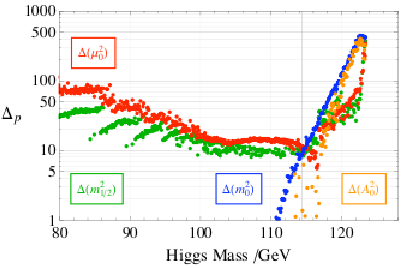
The results obtained are plotted in Figure 1. In the left figure, 2-loop is presented as a function of the Higgs mass. Interestingly, there is a minimum of which predicts a value of which is just above the LEP2 bound, at GeV. The quoted theoretical uncertainty of GeV is due to higher order perturbative corrections that account for differences between the results of SoftSusy and FeynHiggs codes and can be even larger, up to 3 GeV. This value of is found with the above experimental and theoretical constraints, but without imposing the LEP2 bound. It just turns out that minimal fine-tuning wrt to UV parameters indicates a size for the quantum corrections that prefer a total value for close to this bound.
Notice the presence in Figure 1 of the steep, exponential increase of minimal on both sides of its minimum value situated near the LEP2 bound, effect largely due to quantum corrections (note the log OY scale). This behaviour underlines the importance of the minimal value of . Variations of around the central values of and of the top mass, give the results shown by the dotted and dashed lines: a 1 increase of gives very similar results to a 1 decrease of top mass; thus these have opposite effects. Indeed a larger top Yukawa helps a radiative EWSB, while a larger strong coupling has an opposite effect, at two-loop. The minimum of is where these effects are balanced, in other words - assuming minimal , the Higgs mass prediction cannot be larger due to QCD quantum effects. In other words, QCD does not “like” a larger Higgs mass, unless one is prepared to accept the fine tuning cost that comes with it (this is indeed very high for GeV, when one already has ). The conclusion is that, from a 2-loop evaluation of , one finds, rather intriguingly, that minimal favours the value GeV.


|


|


|


|
In the right plot of Figure 1 are shown the individual contributions , ,, , , , to the electroweak fine-tuning . At low , below the LEP2 bound is dominant, while above this bound and at large , is dominant, with reaching similar values near 120 GeV; this contradicts common claims in the literature that is actually the largest and dominant part of , (true only below the LEP2 bound). The transition between the two regions is happening at about 114.5 GeV, shown also in the left plot. With largely related to the EW effects while related to QCD effects, one sees again the significance of the minimal value of overall , at the interplay of these effects. Again, the LEP2 bound is not imposed at any time.
In principle ( is the top Yukawa coupling) could be included in the overall definition of of eq.(2). However, its contribution to is always sub-dominant (relative to ) when assuming the modified definition of [20], appropriate for measured parameters. Under this modified definition one must replace: , where is the 1 error of experimentally measured , in this case . With this modified definition does not change . See also figure 2 in [1] where is actually computed and shown but without the modified definition. The largest for all in the right plot of Figure 1 generates the lower continuous curve of in the left plot in Fig 1.
Let us now put together the short distance (EW/TeV scale) physics effects that we have discussed so far with the large distance physics (dark matter) effects. We therefore analyze the dark matter constraints on CMSSM, whose LSP is a good dark matter candidate. To this purpose, one takes the phase space points in Figure 1, and evaluates for each of them the relic density, , using micrOMEGAs [21] and test if it is consistent with WMAP [4]. The result is presented in Figure 2, where we show the points consistent with the WMAP value as well as those that saturate it within . The plot is very similar for a 1 saturation of WMAP value, with only minor differences. Requiring minimal and consistency with WMAP leads to the predictions:
| (9) |
We checked that using a different definition for , such as of (3) does not change these results for , since is found at similar values for and its plot as a function of with its dark matter constraints is indeed very similar (not shown here). The main difference is an overall shift of the fine-tuning plots of Figure 2 towards higher values of fine tuning, by a factor between 1.5 and 2. The minimum of indicates however the same value of .
To conclude, minimizing the fine-tuning together with the constraints from precision electroweak data, the bounds on Susy masses and the requirement of the observed dark matter abundance lead to a prediction for , without imposing the LEP2 bound, that is marginally above this bound. This is an interesting result, and represents our prediction [1] for the CMSSM lightest Higgs mass based on assuming as a quantitative test of Susy as a solution to the hierarchy problem.
While minimal values of are preferable, one can nevertheless ask what the bounds on the parameter space are, for a beyond which supersymmetry is considered to fail to solve the hierarchy problem. It is in general agreed that this happens for or so. Therefore the bound together with the dark matter consistency (3 upper limit), generates the following upper limits on the CMSSM parameters and :
| (10) |
These values can be re-evaluated for a different upper value of . Note the value of that corresponds to EW fine-tuning of 1 part in 100. Given the exponential increase of with , one sees that at GeV one already has a very large, unacceptable fine-tuning . The mass limits in Table 1 scale approximately as , so they may be adapted depending on how much tuning one is willing to accept.
| 1720 | 305 | 550 | 660 | 665 | 550 | 670 | 2080 | 2660 | 2660 | 3140 |
It is interesting to compare the results in eq.(10) for the parameter space of CMSSM with and dark matter consistency, with the recent exclusion limits of the Atlas/CMS experiments [18, 19], shown in Figure 3. As it can be seen from Figures 4, 5, 6, LHC experiments already probe points in the parameter space that have fine-tuning . Note however that the experimental exclusion curves are for very specific values of the parameters () which are not summed over, and therefore points below these curves that have different values for these parameters are not tested or ruled out.


|
The situation changes for different values of that one is prepared to accept, see the plots in Figures 5 together with the Atlas/CMS exclusion limits. In particular the case with selects points with the smallest fine tuning. It should be stressed that the presence of fewer points (smaller, shrinking area) in the “moduli” space () does not imply anything special for the overall fine-tuning amount, like a larger (disproved by Figures 5). It can for example be related to the quality of the scan of the parameter space. Apart from this, it indicates the most likely values of the parameter (moduli) space that are preferred by the low energy physics, that a fundamental theory (like a string model) should explain or fix dynamically. For related interpretations of the recent LHC results see [23, 24].
It is important to note that most of the region with of the parameter space is being tested by the combined LHC (at 7 TeV) and CDMS-II and Xenon experiments [36], as it was discussed in [22] together with the possible detection signals. Here we only make some comments on the impact of LHC and dark matter experiments on the various regions of the fine-tuning plots shown so far. In figure 6 colour encoding corresponds to the structure of the LSP and shows where points of different are located in the plane . Red points (1) have a low gluino mass, the LSP is mostly bino with a cross section off nuclei too small to be probed by the next generation of direct dark matter searches. Green points (3) have lighter squarks, mostly bino LSP and together with the red points are reachable by LHC run I (right plot). Black points (5) have gluino and squarks near the TeV scale and an almost pure bino LSP. Purple points (2) have a significant higgsino component (), a heavy gluino, ( GeV or larger) and TeV-scale squarks. Although they are not within the reach of LHC run I, they are sensitive to direct dark matter searches; the CDMS II bound is applied in their case while Xenon100 (not applied) can reduce their area further [36]. Also, as seen from the left plot the purple region includes points of very low fine-tuning. In conclusion dark matter and LHC run I searches are rather complementary in covering the entire plane in the TeV region. To cover all the parameter space, beyond will require running at the full 14 TeV CM energy.
3 The impact of “new physics” beyond MSSM on and .
Following this analysis, some natural questions emerge. How do the above predictions for and change under the presence of “new physics” that may exist at some high scale (few TeV or so), beyond the MSSM Higgs sector? Recall that the MSSM Higgs potential is the most minimal construction allowed by supersymmetry, but new physics in this sector can exist: for example extra Higgs doublets, gauge singlets, additional massive U(1)′ bosons, which can all affect the MSSM Higgs sector, its quartic effective coupling and its predictions. Another question is the following: assume for a moment that a Higgs particle is not found at the minimal as discussed above, is it then possible to have a larger , of say 121 GeV but with instead of the corresponding value found above of ?
One answer is that the model considered is too constrained, and this may lead to a large . Indeed, it is known that gaugino universality condition considered here, if relaxed, reduces the value of [25]; another possibility is to relax the universal Higgs mass which can also reduce . Finally, another possibility is that “new physics” missed by the CMSSM Higgs sector, can increase the effective quartic Higgs coupling which leads to a reduction of the fine-tuning amount. The ways to achieve this are numerous but also model dependent.
A simple possibility is to consider the case of MSSM with a low supersymmetry breaking scale ( few TeV ) in the hidden sector [26, 27]. In this case, when integrating out the auxiliary field of the goldstino superfield that is coupled to the MSSM, one generates apart from the usual soft terms, additional quartic terms, without introducing new parameters in the visible sector of the model. Indeed, the scalar potential contains a term [27]
| (11) |
in addition to the MSSM potential, in the standard notation. This term can be significant for low while in the more familiar cases of high scale Susy breaking is strongly suppressed. Such term can help to increase the SM-like Higgs mass at the tree level and reduce since
| (12) |
can be reduced compared to its MSSM counterpart in eq.(8), due to the extra term in the denominator. For more details of this class of models see [27] and references therein.
Other possibilities to increase and reduce can exist, due to “new physics”. To perform a model independent analysis, below we consider an effective theory approach, that parametrizes in a general way the “new physics” that may exist beyond the MSSM Higgs sector. This is done by using a series of effective operators, whose consequences for and are explored below. Let us mention that introducing such operators comes at the cost of having new parameters in the theory, beyond those of the MSSM.
The power of such an effective approach resides in its organizing principle that relies on an expansion in inverse powers of the scale of the ”new physics” that generated these operators. To this purpose we consider the effective operators of dimensions d=5 and d=6 that can exist in the Higgs sector. The reason of considering both classes is twofold: first, the latter can be present as a leading contribution even in the absence of the former. For example integrating out a massive U(1)′ generates d=6 operators, with no d=5 ones. The second reason is that, if generated by the same physics, at large the d=5 operators receive additional suppression and then become of similar order of magnitude to the d=6 operators. In other words, the convergence of the expansion (in ) for large requires one include both classes of operators, when originating from same massive state that was integrated out.
3.1 The case of d=5 operators and their corrections to .
We start with the d=5 operators in the MSSM Higgs sector. There are two of them:
| (13) |
where is the spurion field and we assume so that the expansion is convergent. Here are all dimensionless functions of the spurion that have the form , and similar for and .
can be generated by integrating out a massive gauge singlet or triplet. Let us consider the former case. Indeed, in the MSSM with a massive gauge singlet, with an F-term , when integrating out via the eqs of motion, one generates . This result is similar to considering a generalised NMSSM with a supersymmetric mass term , in the decoupling limit of the singlet. Therefore our results for fine tuning are relevant for the generalised NMSSM model, in this limit.
Regarding , this can be generated in various ways (see Appendix A, B in [28]) but perhaps the simplest way is via an additional pair of massive Higgs doublets of mass of order . However, is actually ”redundant”, since it can be removed by general spurion-dependent field redefinitions, up to soft terms renormalisation, term redefinition and corrections [28]. Therefore plays no role in the following. Note that also includes a particular operator of the form which can be re-written as a Kahler term (for details see [33] and the Appendix in the first work in [2]).


|
Due to the scalar potential acquires additional terms which bring a correction to the effective quartic coupling: . So may increase and as a result we expect that fine-tuning can be reduced. The correction to the MSSM lightest Higgs mass is then
| (14) | |||||
and
| (15) |
for the pseudoscalar Higgs. and are due to and, if present, also operators. The upper (lower) signs correspond to (), and is given by . With this result one can show that the mass can be increased above the LEP2 bound, for low , also with the help of quantum corrections.
Let us now see the amount of fine-tuning as a function of the Higgs mass, in the presence of d=5 operators11 1 There is a subtle point: notice that the RG eqs are not affected at one loop by the presence of a massive gauge singlet that was assumed to generate in the first instance. Therefore this analysis is consistent. The situation is more complicated in the presence of SU(2) triplet; however, the Higgs mass increase and the reduction of fine-tuning due to it remain true, even though the exact value of may be different.. Unlike the MSSM case the analysis of is done at one-loop only, for a sample of points in parameter space with: , TeV, GeV TeV, and GeV, consistent with the signs for chosen so as to reduce the fine tuning. One-loop analytical results for were obtained (for details see [12]), and the corresponding numerical results are shown in Figure 7. Note that in these figures the structure apparent at small and large is a scanning artifact, with the under-dense wedge shaped regions to be filled in with a more dense parameter sample. For a fixed value of and relative to the CMSSM case, one may see a systematic shift towards higher . This is due to an increase of the effective quartic Higgs coupling (which also increases relative to its MSSM value) and, as a result, also decreases . The overall result is that the minimum amount of fine-tuning in the presence of effective operators is reduced relative to the MSSM case, so values of as large as GeV can still have a low . The reduction in the fine tuning at low () relative to the MSSM case is actually much more marked than that shown, given that in the MSSM, in this limit and above the LEP2 bound, actually increases.
Let us examine the scale of new physics needed for this reduction in fine tuning. One has
| (16) |
With between the EW scale and 1 TeV, this shows that large values of are allowed: TeV for GeV, respectively. Also, in this case for GeV. To relax these values one can use that an increase (decrease) of by increases (decreases) by to GeV for the same .
Let us conclude with a remark on fine-tuning in the presence of a massive gauge singlet that was assumed to generate the above operator, and a comparison to the NMSSM case. The above case is less fine tuned than the NMSSM because of the nature of the supersymmetric contribution of the gauge singlet to effective quartic higgs coupling. In our case receives a contribution (see eqs.(14)), while in the NMSSM the corresponding contribution of the singlet is further suppressed, being proportional to . As a result the NMSSM is more fine-tuned (for a similar ). This difference can be further traced back to the absence in NMSSM of a bilinear F-term , that could increase the mass of the singlet significantly (and generated the d=5 operator). Correspondingly, the increase of and thus the reduction of the fine-tuning in NMSSM is not as significant as in the case discussed above (for a fixed ).
3.2 The case of d=6 operators and their correction to .
We can extend the previous discussion to also include the corrections to from effective operators of dimension that can exist beyond the MSSM Higgs sector. Computing the analytical corrections to from individual effective operators is indeed possible. It is however difficult to evaluate the fine tuning in this case, since the operators can be generated in various ways by (unknown) states charged under the SM group, that affect the RG flow of couplings in the model and thus the fine tuning. This is unlike the case of in the case which was assumed to be generated by a massive gauge singlet. Nevertheless, it is obvious that an increase of by the effective operators reduces the fine tuning . For these reasons, in the following we restrict ourselves to computing the corrections to .
| (17) |
where is the chiral field strength of or vector superfields and respectively. Also with the upper sign for . Finally, the wavefunction coefficients are spurion dependent and have the structure
| (18) |
where . can be generated in the MSSM with an additional, massive gauge boson or triplets, when these are integrated out [30]. can be generated by a massive gauge singlet or triplet, while can be generated by a combination of doublets and massive gauge singlet. is essentially a threshold correction to the gauge coupling, with a moduli field replaced by the Higgs, difficult to generate in a renormalisable theory with additional massive states. Finally, exists only in the non-Susy case, but is generated when removing the derivative operator by field redefinitions [28], therefore we keep it. There are also operators which involve derivatives (see later).


|


|
Let us see the implications of these operators for the corrections to the Higgs spectrum. They bring corrections denoted in eq.(14), (15) and their exact expressions can be found in [2, 31]. However, for most purposes, an expansion of these in is accurate enough. At large , operators bring corrections comparable to those of operators. The relative enhancement of corrections compensates for their extra suppression relative to operators. However, in some models only operators may be present, depending on the details of the “new physics” generating the effective operators. If is kept fixed, one finds in order [2] (see also [31]):
| (19) | |||||
The full value of is that obtained by using eq.(19) in (14) where is replaced by the 2-loop leading log value22 2 In the numerical evaluations and figures below we used the exact expression of [2], see also [31].. So the effective operators correction is regarded as a classical correction (“perturbation”) added to the 2-loop leading-log CMSSM value, and crossed-terms that involve products of loop-corrections and effective operators coefficients are neglected, being of higher order. For an easier reading of the effects of the operators, one can introduce the correction
| (20) |
with as in (19). The total Higgs mass value is then . Further, it is preferable to search for possible increases of by supersymmetric rather than supersymmetry-breaking effects of the effective operators, because the latter are less under control in the effective approach33 3 Also, one would prefer a supersymmetric solution to the fine-tuning problem associated with increasing the MSSM Higgs mass well above the LEP2 bound.. In any case, the non-Susy part of the effective operators has an impact on that is comparable to that of the supersymmetric part considered here. So in the following we concentrate only on Susy corrections, induced by the coefficients with to label the corresponding operator .
The results obtained are illustrated in Figures 9, 9 where the correction is shown as a function of the CMSSM value of (2-loop, leading-log). The results are obtained in the the following way. We consider all the phase space points displayed in Figure 2 that respect all experimental and dark matter constraints (except the LEP2 bound on that is not imposed). On this “background” we consider the perturbation due to the effective operators of dimension d=6 and evaluate as outlined above and shown in these figures, as a function of the 2-loop leading-log value of in CMSSM.
From these figures one can conclude that the CMSSM points with lowest fine-tuning corresponding to GeV, have a rather small , of few GeV. For TeV is up to 4 GeV ( GeV for ), and this decreases (increases) by GeV for a 1 TeV increase (decrease) of . However, the value of is usually restricted to be in the region of TeV or higher, from parameter constraints44 4 This bound applies to a combination of operators and can in principle be reduced for individual operators. [32] and our expansion parameter was always taken , where is any scale of the model (, , ). This is considered conservative enough for a convergent perturbative expansion. Note that points which were below the LEP2 bound by the correction mentioned, become now phenomenologically viable. The special point of CMSSM of minimal that saturates the relic density within 3 and with GeV, could receive a correction GeV, so that increases to GeV. Correspondingly, its earlier associated is likely to decrease by a factor proportional to the square of the ratio of the final to the initial value of .
Given the relatively small size of their correction one can say that the particular CMSSM points with and their predictions are rather stable against the presence of supersymmetric “new physics” at the scale TeV. This finding can be explained by the fact that these points generically have a light and also light , and thus the supersymmetric corrections , (, etc) are rather suppressed. The corrections can increase or decrease if one also includes effects of Susy breaking associated to , but these bring additional model dependence and extra parameters.
Let us now discuss about the CMSSM points in Figures 9, 9 with fine tuning , situated above the upper continuous line. They can bring an increase of which can be significant, of 10-30 GeV. For example there are points which for near 100 GeV can receive corrections of order 15-20 GeV, to reach and comply with the LEP2 bound. Interestingly, for the Higgs mass increase is such that total remains close to 122 GeV. Points that are largely fine-tuned and have a value for significantly below the LEP2 bound, are often receiving the largest corrections . This opens the possibility that the phase space of the CMSSM be increased and points which were otherwise ruled out on grounds of extreme fine tuning and/or LEP2 bound, can be “recovered” and become phenomenologically viable.
Finally, notice that we kept all operators independent of each other. By doing so, one can single out the individual contributions of each operator (labelled by ), which helps in model building, since not all operators are present in a specific model. Also it is unlikely that “new physics” will bring up in the leading order, simultaneously, all these operators. What does all this mean for EW scale fine-tuning? The value of for those points initially strongly fine-tuned can decrease by a factor equal to the square of the ratio of the Higgs mass after and before adding the correction and this effect can be significant, as seen earlier for ( case). A similar effect is expected for the case of d=6 operators. So one expects a change of
| (21) |
One cannot obtain a more exact evaluation of in our model-independent approach, i.e. in the absence of the details of the new physics (quantum numbers of massive states) that generated the effective operators in the first instance. For further discussions on this see [2].
3.2.1 Effective operators: removing redundant operators.
The reader may notice that the discussion for the d=6 operators ignored a class of operators that could be present (and that are similar to of the d=5 case). These operators involve extra derivatives and are
| (22) |
Here and is the field strength of . does not depend on Higgs explicitly, but could affect its scalar potential. To be general, in the above operators one should include spurion () dependence under any to account for supersymmetry breaking effects associated to them. Such operators are easily generated when integrating out massive states in 4D models. They can also be generated at one-loop by compactification, after integrating out towers of Kaluza-Klein states, in the presence of localised (Yukawa) interactions [34] (for example , ) or due to bulk (gauge) interactions [35] ().
Such operators are however redundant in the sense that they can be removed by non-linear field redefinitions [2, 28]. To see how this works, consider for example operator , without the gauge field dependence, and in the presence of an otherwise standard Lagrangian, with an arbitrary superpotential :
| (23) |
Here comes from with the replacement . Further, one replaces . This can be unfolded into a “standard” Lagrangian without extra derivatives (see [33], also Appendix B in the first paper in [2]). To see how this works, consider a change of basis to : and where , form an unitary matrix, so that the eigenvalue problem is not changed; is a very small, non-zero mass scale of the theory that can be taken to zero at the end of the calculation. Since and are not independent, such transformation must be accompanied by a Lagrangian constraint, which must vanish in the limit . This constraint has the form:
| (24) |
where is a chiral superfield which plays the role of a Lagrange multiplier, so that the total, equivalent Lagrangian in the new basis is . One then brings to a diagonal form to find the result:
| (25) |
where and where we took the limit . This Lagrangian is that of a second order theory, only polynomial in superfields, and classically equivalent to the initial one (23). Given the signs in the D-term, two massive superghosts () are present, of mass near the effective cut-off, . Their presence is just an effect of truncating the operators series expansion to terms55 5 Indeed, in a renormalisable or ghost-free theory with a massive state, when integrating out this state (by the eqs of motion) one finds in the low-energy effective action an infinite series of derivative terms, suppressed by powers of . The “truncated” theory will have a finite number of derivatives, and, as seen above, this will bring superghosts (or just ghosts in the non-Susy case), i.e. fields with negative kinetic term. This happens even though the theory with the infinite series is ghost-free, since the original theory was so.. Also observe that the field was “spectator” throughout this analysis and did not affect it; in fact the -dependence can be replaced by an arbitrary polynomial function. Further, since the superghost degrees of freedom are massive, one can integrate them out, by the equations of motion. After a careful calculation and consistent Taylor expansion, the result is (see appendix in [2])
| (26) |
where the derivatives of are taken wrt its first argument. This Lagrangian contains only polynomial interactions (renormalisable or not) and standard kinetic terms, and is equivalent to the original one, eq.(23), but has no extra-derivative terms.
This result agrees with that obtained by using the equations of motion in the derivative term in (23), but this is not true in general, as we argue below. Indeed, as shown in the appendix of [2], the presence of a derivative term66 6 Such term is part of discussed in the case of d=5 operators since . in the superpotential of an otherwise arbitrary Lagrangian leads, via the method shown above, to a result that is similar in order to that obtained via the eqs of motion. However, in the the result found by using ordinary eqs of motion is different and actually wrong. The discrepancy is due to the fact that Euler-Lagrange eqs are changed in the higher order theory, and this should be taken into account when using eqs of motion to eliminate the higher-derivative operators. We find the method presented above more elegant and transparent.
Returning to the CMSSM with an additional , the second term in (26) together with the standard MSSM superpotential () can bring only wavefunction renormalization of the Higgs kinetic term or other effective operators polynomial in fields. When Susy breaking is included, such terms also bring soft terms and -term redefinition. A similar strategy applies to the rest of the operators listed in (22). Therefore all these operators are “redundant” in the sense that they can be eliminated, up to redefinitions of the fields, soft masses and -term [28]. For this reason they were not considered in the phenomenological studies of the previous sections.
4 Conclusions
A quantitative test of supersymmetry as a solution to the hierarchy problem is the fine-tuning of the electroweak scale with respect to variations of the UV parameters of the model, after including the quantum corrections and experimental and theoretical constraints. While the largest value of for which Susy is still a solution to this problem is somewhat subjective, it is very natural to ask that be minimal in a given model. This point of view is also supported in part by Bayesian approaches to data fits, in which is automatically included in the effective prior expression as an extra factor, so that the method brings naturally a fine-tuning penalty for points of large . This underlines the physical meaning of in general and the need of minimizing the overall fine-tuning as done in this work, to select the points of physical relevance.
We applied this idea of minimizing to the CMSSM at two-loop leading log, and investigated its results for the value of the radiatively corrected value of the lightest Higgs mass, . Remarkably, although depends exponentially on , there does exist a minimum at a very acceptable value () corresponding to a mass GeV. The very existence of such a minimum situated at the intersection of two exponential dependences on both sides of this value for , and induced by quantum corrections, cannot be stressed enough. The exponential growth of for above this value is largely due to QCD quantum effects which overcome the “good” Yukawa loop effects needed to induce radiative EW symmetry breaking. Thus QCD “does not like” a larger unless one is prepared to pay the associated (high) fine-tuning cost. Imposing consistency with the WMAP bound, the above value changes mildly to leading to GeV, while saturating this bound within 3 leads to with GeV (the quoted theoretical uncertainty ( GeV) can actually be larger, up to GeV).
It is indeed remarkable that constraints from short distance physics (EW precision data) and from large distance physics (dark matter) can be consistent with each other so accurately, and together can help one to make physical predictions. We also checked that using a different definition for , such as does not change this result for , since is found at similar values for and its plot as a function of is very similar. Finally, let us note that points with are currently being tested by the LHC 7 TeV run and by dark matter experiments (CDMS, Xenon, etc) and their impact was briefly discussed.
We further discussed how the results for and change under the addition of “new physics” beyond the MSSM Higgs sector and also whether one could have a larger with a low . This is relevant for MSSM since for GeV, is already , and becomes 1000 for GeV! The “new physics” could reduce to acceptable values, even at larger . It could be represented by additional Higgs doublets, massive gauge singlets or massive U(1)′, etc, and its effects can be generally parametrized by series of effective operators, suppressed by the scale of massive states that generated them. We considered both d=5 and d=6 operators. In the presence alone of the former, one can achieve a low even for as large as GeV. Such a effective operator can be generated by integrating out a massive gauge singlet beyond MSSM, whose effect is to increase the quartic higgs coupling and reduce the fine tuning for similar . This case is nothing but the decoupling limit of the generalised NMSSM which contains a supersymmetric mass term for the gauge singlet (in ordinary NMSSM, the fine tuning reduction is smaller). Other ways to generate such operator can however exist.
Regarding the operators of dimension d=6, we considered their individual, supersymmetric corrections to the CMSSM 2-loop leading log value of , for an expansion parameter with any scale of the model . Their effects were treated as a perturbation of the CMSSM “background” points that respected all experimental constraints. It was shown that CMSSM points with having GeV (, GeV) receive supersymmetric corrections of up to 4 (6) GeV from individual operators, respectively. Therefore, the points in the CMSSM of lowest fine-tuning receive rather modest (supersymmetric) corrections from individual operators, and are therefore rather stable under ”new physics” at a scale considered here of 8 TeV. Applied to the point of minimal fine tuning (GeV), the correction mentioned of 4(6) GeV from individual d=6 operators brings up to a value of GeV. Including a 3 consistency with WMAP changes this result mildly up to GeV. Finally, an increase (decrease) of the scale by 1 TeV brings a decrease (increase) of the correction by about 1 GeV. A next step in this study is to impose dark matter constraints on the CMSSM with d=6 operators, since by supersymmetry these extend the neutralino sector too. The obtained bounds on can then be used to re-evaluate the quoted correction to in the presence of these operators.
Acknowledgments
The work of SC was supported by the UK Science and Technology Facilities Council under contract PPA/S/S/2006/04503. This work was supported in part by a grant of the Romanian National Authority for Scientific Research, CNCS – UEFISCDI, project number PN-II-ID-PCE-2011-3-0607.
References
- [1] S. Cassel, D. M. Ghilencea and G. G. Ross, “Testing SUSY at the LHC: Electroweak and Dark matter fine tuning at two-loop order,” Nucl. Phys. B 835 (2010) 110. [arXiv:1001.3884 [hep-ph]]. “Testing SUSY,” Physics Letters B 687 (2010) 214.
- [2] I. Antoniadis, E. Dudas, D. M. Ghilencea and P. Tziveloglou, “MSSM Higgs with dimension-six operators,” Nucl. Phys. B 831 (2010) 133. [arXiv:0910.1100 [hep-ph]]. “Beyond the MSSM Higgs with d=6 effective operators,” Nucl. Phys. B 848 (2011) 1 [arXiv:1012.5310 [hep-ph]].
- [3] J. R. Ellis, K. Enqvist, D. V. Nanopoulos and F. Zwirner, “Observables In Low-Energy Superstring Models,” Mod. Phys. Lett. A 1 (1986) 57. R. Barbieri and G. F. Giudice, “Upper Bounds On Supersymmetric Particle Masses,” Nucl. Phys. B 306 (1988) 63;
- [4] G. Hinshaw et al. [WMAP Collaboration], “Five-Year Wilkinson Microwave Anisotropy Probe (WMAP) Observations:Data Processing, Sky Maps, & Basic Results,” Astrophys. J. Suppl. 180 (2009) 225 [arXiv:0803.0732 [astro-ph]].
- [5] See for example: S. S. AbdusSalam, B. C. Allanach, F. Quevedo, F. Feroz and M. Hobson, “Fitting the Phenomenological MSSM,” Phys. Rev. D81 (2010) 095012. [arXiv:0904.2548 [hep-ph]].
- [6] B. C. Allanach, “Naturalness priors and fits to the constrained minimal supersymmetric standard model,” Phys. Lett. B635 (2006) 123-130. [hep-ph/0601089].
- [7] M. E. Cabrera, J. A. Casas, R. Ruiz de Austri, “Bayesian approach and Naturalness in MSSM analyses for the LHC,” JHEP 0903, 075 (2009). [arXiv:0812.0536 [hep-ph]]. “MSSM Forecast for the LHC,” JHEP 1005 (2010) 043. [arXiv:0911.4686 [hep-ph]].
- [8] S. P. Martin and M. T. Vaughn, “Two Loop Renormalization Group Equations For Soft Supersymmetry Breaking Couplings,” Phys. Rev. D 50, 2282 (1994) [Erratum-ibid. D 78, 039903 (2008)] [arXiv:hep-ph/9311340].
- [9] M. S. Carena, J. R. Espinosa, M. Quiros and C. E. M. Wagner, “Analytical expressions for radiatively corrected Higgs masses and couplings in the MSSM,” Phys. Lett. B 355 (1995) 209 [arXiv:hep-ph/9504316].
- [10] R. Barate et al. [LEP Working Group for Higgs boson searches], “Search for the standard model Higgs boson at LEP,” Phys. Lett. B 565, 61 (2003) [arXiv:hep-ex/0306033]; S. Schael et al. [ALEPH Collaboration], “Search for neutral MSSM Higgs bosons at LEP,” Eur. Phys. J. C 47, 547 (2006) [arXiv:hep-ex/0602042.
- [11] J. A. Casas, J. R. Espinosa and I. Hidalgo, “The MSSM fine tuning problem: A way out,” JHEP 0401 (2004) 008 [arXiv:hep-ph/0310137]; “A relief to the supersymmetric fine tuning problem,” [arXiv:hep-ph/0402017].
- [12] S. Cassel, D. M. Ghilencea and G. G. Ross, “Fine tuning as an indication of physics beyond the MSSM,” Nucl. Phys. B 825 (2010) 203 [arXiv:0903.1115 [hep-ph]].
- [13] S. Dimopoulos and G. F. Giudice, “Naturalness constraints in supersymmetric theories with nonuniversal soft terms,” Phys. Lett. B 357 (1995) 573 [arXiv:hep-ph/9507282].
- [14] P. H. Chankowski, J. R. Ellis and S. Pokorski, “The fine-tuning price of LEP,” Phys. Lett. B 423 (1998) 327 [arXiv:hep-ph/9712234].
- [15] P. H. Chankowski, J. R. Ellis, M. Olechowski and S. Pokorski, “Haggling over the fine-tuning price of LEP,” Nucl. Phys. B 544 (1999) 39 [arXiv:hep-ph/9808275].
- [16] B. C. Allanach, “SOFTSUSY: A C++ program for calculating supersymmetric spectra,” Comput. Phys. Commun. 143 (2002) 305 [arXiv:hep-ph/0104145].
- [17] The Tevatron Electroweak Working Group (TevEWWG) and CDF Collaboration and D0 Collab, “A Combination of CDF and D0 Results on the Mass of the Top Quark,” [arXiv:0803.1683 [hep-ex]].
- [18] J. B. G. da Costa et al. [Atlas Collaboration], “Search for squarks and gluinos using final states with jets and missing transverse momentum with the ATLAS detector in sqrt(s) = 7 TeV proton-proton collisions,” arXiv:1102.5290 [hep-ex].
- [19] G. Aad et al. [ATLAS Collaboration], “Search for squarks and gluinos using final states with jets and missing transverse momentum with the ATLAS detector in sqrt(s) = 7 TeV proton-proton collisions,” arXiv:1109.6572 [hep-ex].
- [20] P. Ciafaloni and A. Strumia, “Naturalness upper bounds on gauge mediated soft terms,” Nucl. Phys. B 494 (1997) 41 [arXiv:hep-ph/9611204];
- [21] G. Belanger, F. Boudjema, A. Pukhov and A. Semenov, “micrOMEGAs2.0: A program to calculate the relic density of dark matter in a generic model,” Comput. Phys. Commun. 176, 367 (2007) [arXiv:hep-ph/0607059].
- [22] S. Cassel, D. M. Ghilencea, S. Kraml, A. Lessa, G. G. Ross, “Fine-tuning implications for complementary dark matter and LHC SUSY searches,” [arXiv:1101.4664 [hep-ph]].
- [23] B. C. Allanach, T. J. Khoo, C. G. Lester, S. L. Williams, “The impact of the ATLAS zero-lepton, jets and missing momentum search on a CMSSM fit,” [arXiv:1103.0969 [hep-ph]].
- [24] O. Buchmueller, R. Cavanaugh, D. Colling, A. De Roeck, M. J. Dolan, J. R. Ellis, H. Flacher, S. Heinemeyer et al., “Implications of Initial LHC Searches for Supersymmetry,” [arXiv:1102.4585 [hep-ph]]. S. Cassel, D. M. Ghilencea, S. Kraml, A. Lessa, G. G. Ross, “Fine-tuning implications for complementary dark matter and LHC SUSY searches,” [arXiv:1101.4664 [hep-ph]]. S. Akula, N. Chen, D. Feldman, M. Liu, Z. Liu, P. Nath and G. Peim, “Interpreting the First CMS and ATLAS SUSY Results,” arXiv:1103.1197 [hep-ph]. D. Feldman, K. Freese, P. Nath, B. D. Nelson and G. Peim, “Predictive Signatures of Supersymmetry: Measuring the Dark Matter Mass and Gluino Mass with Early LHC data,” arXiv:1102.2548 [hep-ph]. P. Bechtle, K. Desch, H. K. Dreiner, M. Kramer, B. O’Leary, C. Robens, B. Sarrazin, P. Wienemann, “What if the LHC does not find supersymmetry in the sqrt(s)=7 TeV run?,” [arXiv:1102.4693 [hep-ph]]. S. Akula, D. Feldman, Z. Liu, P. Nath, G. Peim, “New Constraints on Dark Matter from CMS and ATLAS Data,” [arXiv:1103.5061 [hep-ph]]
- [25] G. L. Kane, S. F. King, “Naturalness implications of LEP results,” Phys. Lett. B451 (1999) 113 [arXiv:hep-ph/9810374]; D. Horton and G. G. Ross, “Naturalness and Focus Points with Non-Universal Gaugino Masses”, Nucl.Phys.B830 (2010) 221, arXiv:0908.0857 [hep-ph].
- [26] A. Brignole, J. A. Casas, J. R. Espinosa and I. Navarro, “Low-scale supersymmetry breaking: Effective description, electroweak breaking and phenomenology”, Nucl. Phys. B 666 (2003) 105 [arXiv:hep-ph/0301121].
- [27] I. Antoniadis, E. Dudas, D. M. Ghilencea and P. Tziveloglou, “Non-linear MSSM,” Nucl. Phys. B 841 (2010) 157 [arXiv:1006.1662 [hep-ph]].
- [28] I. Antoniadis, E. Dudas, D. M. Ghilencea and P. Tziveloglou, “MSSM with Dimension-five Operators,” Nucl. Phys. B 808 (2009) 155 [arXiv:0806.3778 [hep-ph]].
- [29] D. Piriz and J. Wudka, “Effective operators in supersymmetry,” Phys. Rev. D 56 (1997) 4170 [arXiv:hep-ph/9707314].
- [30] M. Dine, N. Seiberg and S. Thomas, “Higgs Physics as a Window Beyond the MSSM (BMSSM),” Phys. Rev. D 76 (2007) 095004 [arXiv:0707.0005 [hep-ph]].
- [31] M. Carena, K. Kong, E. Ponton and J. Zurita, “Supersymmetric Higgs Bosons and Beyond,” Phys. Rev. D 81 (2010) 015001 [arXiv:0909.5434 [hep-ph]]. M. Carena, E. Ponton, J. Zurita, “BMSSM Higgs Bosons at the Tevatron and the LHC,” Phys. Rev. D82 (2010) 055025. [arXiv:1005.4887 [hep-ph]]. “BMSSM Higgs Bosons at the 7 TeV LHC,” [arXiv:1111.2049 [hep-ph]].
- [32] K. Blum, C. Delaunay and Y. Hochberg, “Vacuum (Meta)Stability Beyond the MSSM,” Phys. Rev. D 80 (2009) 075004 [arXiv:0905.1701 [hep-ph]].
- [33] I. Antoniadis, E. Dudas and D. M. Ghilencea, “Supersymmetric Models with Higher Dimensional Operators,” JHEP 0803 (2008) 045 [arXiv:0708.0383 [hep-th]].
- [34] D. M. Ghilencea, “Higher derivative operators as loop counterterms in one-dimensional field theory orbifolds,” JHEP 0503 (2005) 009 [arXiv:hep-ph/0409214]. D. M. Ghilencea and H. M. Lee, “Higher derivative operators from transmission of supersymmetry breaking on S(1)/Z(2),” JHEP 0509 (2005) 024 [arXiv:hep-ph/0505187].
- [35] S. Groot Nibbelink and M. Hillenbach, “Renormalization of supersymmetric gauge theories on orbifolds: Brane gauge couplings and higher derivative operators,” Phys. Lett. B 616 (2005) 125 [arXiv:hep-th/0503153]. D. M. Ghilencea, “Compact dimensions and their radiative mixing,” Phys. Rev. D 70 (2004) 045018 [arXiv:hep-ph/0311264]. S. G. Nibbelink and M. Hillenbach, “Quantum corrections to non-Abelian SUSY theories on orbifolds,” Nucl. Phys. B 748 (2006) 60 [arXiv:hep-th/0602155]. D. M. Ghilencea, H. M. Lee and K. Schmidt-Hoberg, “Higher derivatives and brane-localised kinetic terms in gauge theories on orbifolds,” JHEP 0608 (2006) 009 [arXiv:hep-ph/0604215].
- [36] Z. Ahmed et al. [ The CDMS-II Collaboration ], “Dark Matter Search Results from the CDMS II Experiment,” Science 327 (2010) 1619-1621. [arXiv:0912.3592 [astro-ph.CO]]. E. Aprile et al. [ XENON100 Collaboration ], “Dark Matter Results from 100 Live Days of XENON100 Data,” Phys. Rev. Lett. 107 (2011) 131302. [arXiv:1104.2549 [astro-ph.CO]].