Robust Lattice Alignment for -user MIMO Interference Channels with Imperfect Channel Knowledge
Abstract
In this paper, we consider a robust lattice alignment design for -user quasi-static MIMO interference channels with imperfect channel knowledge. With random Gaussian inputs, the conventional interference alignment (IA) method has the feasibility problem when the channel is quasi-static. On the other hand, structured lattices can create structured interference as opposed to the random interference caused by random Gaussian symbols. The structured interference space can be exploited to transmit the desired signals over the gaps. However, the existing alignment methods on the lattice codes for quasi-static channels either require infinite SNR or symmetric interference channel coefficients. Furthermore, perfect channel state information (CSI) is required for these alignment methods, which is difficult to achieve in practice. In this paper, we propose a robust lattice alignment method for quasi-static MIMO interference channels with imperfect CSI at all SNR regimes, and a two-stage decoding algorithm to decode the desired signal from the structured interference space. We derive the achievable data rate based on the proposed robust lattice alignment method, where the design of the precoders, decorrelators, scaling coefficients and interference quantization coefficients is jointly formulated as a mixed integer and continuous optimization problem. The effect of imperfect CSI is also accommodated in the optimization formulation, and hence the derived solution is robust to imperfect CSI. We also design a low complex iterative optimization algorithm for our robust lattice alignment method by using the existing iterative IA algorithm that was designed for the conventional IA method. Numerical results verify the advantages of the proposed robust lattice alignment method compared with the TDMA, two-stage ML decoding, generalized Han-Kobayashi (HK), distributive IA and conventional IA methods in the literature.
Index Terms:
lattice codes, interference alignment, interference channel, MIMO, imperfect CSII Introduction
Interference is a fundamental bottleneck in wireless systems. This is partially due to the lack of understanding interference from an information theoretic view. For example, the capacity region of the two-user Gaussian interference channels has been an open problem for over 30 years. It was only shown recently that the Han-Kobayashi (HK) achievable region [1] achieves the capacity region to within one bit[2]. Lately, there have been some breakthroughs on the understanding of -user interference channels. In [3] and [4], the authors propose an interference alignment (IA) method to align interference onto a lower dimensional subspace of each receiver so that the desired signal can be transmitted on the interference-free dimensions. The authors show that IA is optimal in the degrees-of-freedom (DoF) sense (which is a high SNR performance measure) and the total capacity of the -user interference channels is given by [3]. There are a number of extensions [5, 6] that have studied the application of IA in -user quasi-static MIMO interference channels. However, the conventional IA method for -user interference channels requires infinite dimension in time-varying or frequency-selective channels, and has the feasibility problem. For example, it is shown in [7] that conventional IA in quasi-static MIMO ( transmit and receive antennas) interference channels is not able to achieve a per user DoF greater than . As a result, there is no satisfactory solution for quasi-static MIMO interference channels for large due to the feasibility problem.
Besides the feasibility problem, conventional IA solutions have assumed Gaussian input symbols and it is unclear whether it is optimal to employ Gaussian input for interference channels. With the Gaussian input symbols, the interference space is random and all the conventional IA methods try to align all interference to a smaller dimension space and utilize the remaining interference-free dimensions to transmit the desired signals. While Gaussian inputs (using random codebook argument) are capacity optimal in multi-access and broadcast channels[8, 9], they are not optimal for interference channels [10, 2]. It is revealed in [10] that structured interference is more preferred in interference networks. Instead of giving up the space that is reserved for the interference and transmitting the desired signal on the remaining interference-free dimensions, one could also exploit the structured interference space and transmit desired signals over the gaps. This motivates the lattices based study of interference alignment. In [11, 12], the authors propose a lattice interference alignment method to align the interfering lattices on a common basis but it only works for symmetric SISO interference channels (where all cross links have the same fading coefficients) or a specialized class of 3-user SISO interference channels (where the products of the fading coefficients are assumed to be rational). In [13, 14], the authors propose interference alignment over real line for -user quasi-static MIMO interference channels with real channel coefficients and demonstrate that the DoF can be achieved. This approach is further extended to the complex channel in [15] for the compound MIMO broadcast channel. In addition to interference channels, lattice codes have also been widely studied in many communication networks [16] such as point-to-point channels and wireless relay networks. Specifically, in [17], the author shows that lattice codes can achieve the capacity of in the point-to-point additive white Gaussian noise (AWGN) channel. In [18], the authors exploit the lattice codes and propose a compute-and-forward method in wireless relay networks. They show that each relay can decode a linear function of messages from multiple source nodes by using lattice codes. A destination node can decode the desired message, given sufficient linear combinations forwarded from the relay nodes.
All these results indicate that we can potentially benefit from the structured interference created by lattice codes. However, in order to have a practical method for exploiting the advantage of the structured interference due to lattice transmissions, there are still some key technical challenges to be addressed.
- •
How to align the received lattices on a common basis over irrational quasi-static MIMO interference channels: Creating an ideal structured interference space [11, 12] requires that all the interfering lattices to be received on a common basis at each of the receivers. However, this is a difficult requirement and is impossible for irrational fading matrices. While [11, 12] study lattice alignment methods for user quasi-static interference channels, the methods therein only work for symmetric interference channels or a specialized class of 3-user SISO interference channels. These approaches cannot be used for general non-symmetric irrational interference channels.
- •
How to exploit structured interference at finite SNR: In [13, 14], the authors propose a lattice alignment algorithm for MIMO interference channels, which is optimal in the DoF sense. However, it is not known whether this approach can be applied at finite SNR, which is an important operating regime in practice. In [19], the authors propose an ergodic interference alignment method which could work at finite SNR regime. However, it requires either infinite time or frequency extension and cannot be applied for constant channels.
- •
How to ensure robustness due to imperfect knowledge of CSI: All of the above works assume perfect knowledge of channel state information (CSI) for facilitating interference alignment. In practice, this is not possible and interference alignment performs very poorly with imperfect CSI [20]. It is quite challenging to incorporate robustness with respect to (w.r.t.) imperfect CSI and exploit the structured interference space at the same time.
In this paper, we explore a robust precoder and decorrelator design for -user general irrational quasi-static MIMO interference channels with imperfect CSI. We propose a robust lattice alignment method (which does not have the feasibility problem) for general irrational constant interference channels, and deduce a two-stage decoding algorithm to decode the desired signal from the structured interference space. We derive the achievable data rate based on the proposed method and formulate the precoders, decorrelators, scaling coefficients as well as the interference quantization coefficients11 1 Please refer to Section IV for details about these design parameters. design as a mixed integer and continuous optimization problem [21]. By utilizing the alternating optimization technique and by exploiting the structured interference, we derive a low complexity algorithm to determine the precoders, decorrelators as well as the interference quantization coefficients. The effect of imperfect CSI is also accommodated in the optimization formulation and hence, the derived solution is robust to imperfect CSI. To illustrate the benefit of the proposed method, we compare the achievable data rates with those of the conventional IA method [3], the distributed IA method based on alternating optimization [5], the TDMA method, the brute-force two-stage maximum likelihood (ML) decoding method and the generalized HK method [1, 2] with random Gaussian input symbols. We show that the proposed method achieves the same DoF as the conventional IA method if the problem is feasible. On the other hand, when the conventional IA is not feasible, our proposed solution can still offer significant performance gain compared with these baselines.
This paper is organized as follows. In Section II, we outline the system model of the -user quasi-static MIMO interference channels. In Section III, we review some common interference alignment methods in the literature and provide some preliminary discussions on the lattices. In Section IV, we propose the robust lattice alignment method and formulate it as a mixed integer and continuous optimization problem. In Section V, by using the alternating optimization technique, we derive a low complexity solution. In Section VI, we derive closed-form analysis of the proposed method and the baseline methods under specialized channel realizations. The performance of the proposed method and the existing methods under complex channel realizations is illustrated in Section VII. We conclude with a brief summary of the results in Section VIII.
II System Model
II-A -user Quasi-Static MIMO Interference Channels
We consider the -user quasi-static MIMO Gaussian interference channels as illustrated in Fig. 1. Each transmitter, equipped with antennas, tries to communicate to its corresponding receiver, which is equipped with antennas. Specifically, we consider a block of channel symbols. The channel output at the -th receiver is described as follows:
| (1) |
where, is the MIMO complex fading coefficients from the -th transmitter to the -th receiver. is the complex signal vector transmitted by transmitter . is the circularly symmetric AWGN vector at receiver . We assume all noise terms are i.i.d. zero mean complex Gaussian with unit variance.

II-B Precoding at Transmitters
In this paper, we assume that each transmitter transmits independent data streams. Specifically, is the precoder for the -th complex data stream () at transmitter . Therefore, . The average power for each data stream is given by . The precoders are chosen such that the total transmit power for each transmitter is no more than , i.e.,
| (2) |
where .
II-C Imperfect Channel State Information Model
The imperfect CSI model can be expressed as:
| (3) |
where is the estimated CSI that is known at the central coordinator. is the CSI error satisfying:
| (4) | |||||
This deterministic channel estimation error model is widely used in the literature [22, 23, 24]. Therefore, given the estimated CSI , the uncertainty of is an ellipsoid centered at with radius .
III Summary of the Existing Interference Alignment Methods and Lattices
III-A Interference Alignment on a Quasi-Static MIMO Space
It is shown in [3] that in the 3-user quasi-static MIMO interference channels with antennas, DoF can be achieved. Specifically, when is even, each transmitter sends independent streams over the precoder for transmitter , i.e.,
| (5) |
The precoders are designed in terms of the channel matrices, where the dimension of the interference space is equal to at each receiver. Each receiver can simply cancel the interference by zero-forcing and then decode the desired streams. When is odd, similar results can be obtained by considering a two time-slot symbol extension of the channel, with the same channel coefficients over the two symbols. However, it is shown in [7] that the above method is not able to achieve a per user DoF greater than .
III-B Interference Alignment on a Lattice
In [12], the authors consider IA on a lattice for some special 3-user SISO interference channels . Specifically, the real channel fading coefficients have to satisfy the following requirement:
| (6) |
where and are integers such that . is the greatest common divider of the integers. Transmitter chooses the lattice generated by using construction A described in [25]. In order to align the interfering lattices at each receiver, the lattices are chosen by:
| (7) |
As a result, a two-stage decoding algorithm can be done at each receiver, which decodes the aggregate interference first and then subtracts the aggregate interference from the received signal to decode the desired information. Note that the symmetric channel considered in [11] is a special case in (6). This method requires strong interference channels to decode the interference first (treating the desired signal as additive noise). Furthermore, the requirement of adding the interfering lattice on a common basis at each receiver as in (7) becomes infeasible for general irrational -user quasi-static interference channels. A simple counter example is given below.
Example 1 (A Simple Counter Example)
A simple counter example is given by: . It is not possible to align the interfering lattices on a common basis at each of the 3 receivers. ∎
III-C Interference Alignment over the Real Line
It is shown in [14] that DoF can be achieved for quasi-static MIMO using IA on the real line [13]. This approach is extended to the complex channel in [15] for the compound MIMO broadcast channel. Here we review the basic idea for the SISO interference channels in [13], and it is easy to extend to the MIMO case as in [14, 15]. Specifically, the received signal at receiver can be represented as [13]
| (8) |
where controls the input power of all users. is one of the integers in the set , and carries information for the -th data stream for user . is a constant real number, which is the direction of the transmitted -th data stream. It is chosen as monomials with variables from channel coefficients. is the aggregated interference caused by all users. The data streams are aligned if they arrive at the same direction. e.g., interference and are aligned at receiver 3 if . By carefully designing the transmit directions, it is shown in [13, 14] that DoF can be achieved. However, this method requires infinite SNR and it is not known if this method could be modified for finite SNR regime.
III-D Lattices
In this section, we shall review some preliminaries on lattices from [18, 16] and the references therein. A -dimensional lattice is a set of points in , and is given in terms of the lattice generator matrix :
| (9) |
A lattice quantization is a function, , that maps a point to the nearest lattice point in Euclidean distance:
| (10) |
The fundamental Voronoi region, , of , is the set of points in closest to the zero vector, i.e., . The modulo- operation w.r.t. the lattice is defined as
| (11) |
which is also the quantization error of w.r.t. .
A nested lattice code is the set of all points of a fine lattice that are within the fundamental Voronoi region of a coarse lattice :
| (12) |
where is said to be nested in , i.e., . Please refer to Fig. 2 in [18] for an illustration of nested lattice. The rate of a nested lattice code is given by:
| (13) |
where is the volume of .
IV Robust Lattice Alignment
In this section, we introduce the framework of our robust lattice alignment method and the associated two-stage decoding algorithm. We derive the minimum achievable data rate and design the precoder, decorrelator and the interference quantization coefficients via an optimization approach.
IV-A Encoding at Transmitters
In this paper, we adopt the lattice encoding method, which is used both in point-to-point channels [17] and relay networks [18]. Specifically, the data stream is given by:
| (14) |
where is the coarse lattice used in the nested lattice encoding method for the transmitted symbols . are points in the nested lattice code (corresponding to the fine lattice ) that carry information. are the dither vectors [17, 18] which are independently uniformly distributed over and are available to all transmitters and receivers. Specifically, all the nested lattices are AWGN good, and the coarse lattice is quantization good22 2 Please refer to [16] for the definition of goodness for lattice codes. Specifically, the lattice codes should have both good statistical and good algebraic properties[18].. In [18], such lattices and dither vectors satisfying the transmit power constraint are proved to exist.
Remark 1 (Complexity of the Encoding Method)
The complexity of the encoding method is similar to that in the baselines. In the baseline methods, standard Gaussian random codebook is assumed to achieve the mutual information rate. On the other hand, there exists efficient coding schemes by using a scalar constellation coupled with a linear code and this could come close to the nested lattice performance (without the shaping gain)[26]. ∎
Note that, dithering is a common randomization technique in lattice quantization for source coding [17]. The following two lemmas from [17, 18] capture the key properties of the dithered nested lattice codes.
Lemma 1 (Erez-Zamir[17])
For any random variable , if is statistically independent of and uniformly distributed over , is uniformly distributed over , and is statistically independent of . ∎
Lemma 2 (Nazer-Gastpar[18])
Let and be statistically independently uniformly distributed over with , and for some constant and . The density of is upper bounded by the density of an i.i.d. zero-mean Gaussian vector whose variance approaches as , where . ∎
IV-B Lattice Alignment with Imperfect CSI
In this section, we shall discuss the proposed robust lattice alignment method (using vector space strategies) and the motivations. When Gaussian signals are transmitted in interference channels, the associated interference space is random as illustrated in Fig. 2[10]. Intuitively, the aggregate interference will fill the entire signal space and there is no room left for desired signal transmission. Furthermore, the penalty of interference scales with the number of interferers. As a result, the key idea behind the IA methods in [3, 4] is to align all interferences to a lower dimensional subspace and utilize the remaining interference free dimensions to transmit the desired signals. However, one problem associated with the IA method in [3, 4] is the feasibility problem. In fact, it is shown in [7] that the per user DoF greater than is not achievable.
On the other hand, when structured lattices are used at the transmitters, the aggregate interference at each of the receiver may be structured (if the interfering lattices are properly aligned) as illustrated in Fig. 2[10]. In this case, the interference space contains regular gaps that can be utilized to transmit desired signals. More importantly, the penalty of the interference does not scale with the number of interferers. Therefore, another possible direction of alignment is to align the transmit lattices on a common basis at each of the receivers to create a structured interference space as illustrated in Fig. 2[10]. However, it is not always possible to simultaneously align all the interfering lattices, as shown in Example 1. Furthermore, perfect lattice alignment requires perfect CSI, which is impractical.

Motivated by the advantages of having structured interference, we propose a robust lattice alignment method in which the precoders are designed to align the received lattices as much as possible. We accept the fact that lattice alignment may not be perfect (due to infeasible irrational channel coefficients and imperfect CSI) and we try to minimize the effect of the residual lattice alignment error. Specifically, instead of decoding and subtracting each interference individually, we wish to decode the structured aggregate interference composed of all the interferences and remove them all at once. Furthermore, due to the structural constraints of the lattice, we must choose integer coefficient for each data stream to approximate the equivalent channel coefficient. Therefore, the aggregate interference lattice for the data stream is written as:
| (15) |
where (complex integer) is defined as the interference quantization coefficient to approximate the equivalent channel coefficient for , and (see Fig. 3 for an illustration). Specifically, given the precoder for , the decorrelator at receiver , and the interference quantization coefficients , the alignment error is given by:
| (16) |

Remark 3 (The Effect of Design Parameters on )
Based on the aggregate interference lattice in (15), a two-stage decoding algorithm can be constructed at each of the receivers as illustrated in Fig. 4. The first stage is to decode the structured aggregate interference, whereas the second stage is to decode the desired signal after canceling the decoded aggregate interference. The decoding process and the associated error analysis in the presence of the residual alignment errors are discussed in detail in the following subsections.
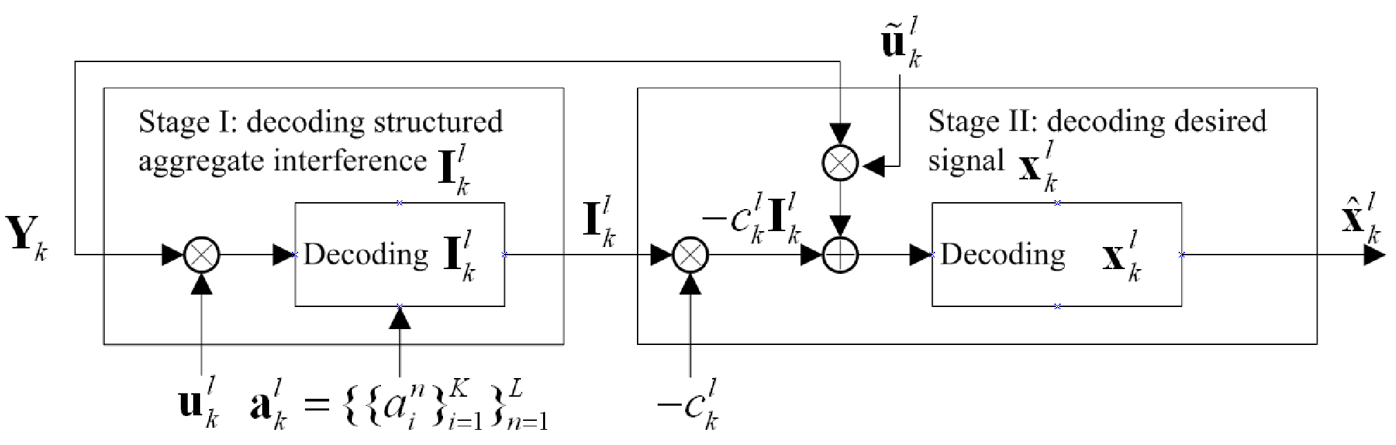
IV-C Stage I - Decoding the Aggregate Interference
| (17) |
| (18) |
Note that the received signal at the -th receiver is given by:
| (19) |
At stage I, a complex linear decorrelator () is applied at receiver , i.e.,
| (20) |
From (), we wish to decode the structured aggregate interference, i.e.,
| (21) |
where , and . Let denote the interference quantization coefficients for decoding the desired data stream . and denote the real and imaginary parts, respectively. To successfully decode , there are some requirements on the transmit data rates of the streams in the term. The achievable rate region of the users for successful stage I decoding under the imperfect CSI model in (4) is summarized in Lemma 3.
Lemma 3
(A Sufficient Condition for Successful Stage I Decoding under Imperfect CSI): Under the imperfect CSI model in (4), the structured aggregate interference can be decoded from with arbitrarily small error probability if the data rate satisfies the condition (for all ) given in (17), where means the product of the two terms . ∎
Proof:
Please refer to Appendix A. Note that a similar result with perfect CSI is derived in [18] for single-stream wireless relay networks. ∎
Note that when for all , i.e., , there will be no stage I decoding for the desired data stream and the proposed method reduces to the conventional precoder-decorrelator optimization with one-stage decoding. The first term and the second term in the denominator of (17) correspond to the noise term and the residual lattice alignment errors, respectively.
IV-D Stage II - Decoding the Desired Signal
After successfully decoding the structured aggregate interference at stage I, we wish to decode the desired signal at stage II. This is illustrated in Fig. 4. Specifically, the scaled structured aggregate interference is subtracted from the received signal and the desired signal is decoded via given by:
where is the second stage decorrelator, is the scaling coefficient33 3 We may need to scale the decoded aggregate interference first before subtracting from the received signal so as to compensate for the amplitude change due to the second stage decorrelator . for the -th data stream at receiver , is the -function (all except ), and
| (25) |
where follows from for all , follows from and for all . Similarly, we have
| (26) |
From (IV-D) note that, if we set , then , and hence the stage II decoding in (IV-D) would try to directly null off the interference . Similarly, the sufficient condition in terms of the rate region for successful stage II decoding is given in the next lemma:
Lemma 4
Proof:
The proof follows from a similar approach as in Appendix A. Specifically, it is obtained by replacing and (obtained from (25) and (26)) with and in the proof of Lemma 3, respectively. Note that, from (25) and (26), the equivalent channel coefficient for data stream in stage II decoding is . Furthermore, since we wish to decode , in (18) indicates the coefficient for and the coefficients for the other data streams are all 0. ∎
Note that the rate region in (18) is a function of interference quantization coefficients , scaling coefficients , precoders , and second stage decorrelators .
Remark 4 (Complexity of the Decoding Method)
The decoding complexity of the proposed design and the baselines are similar. For instance, all baseline methods have assumed ML decoding to achieve the mutual information rate. On the other hand, there exists efficient lattice decoding methods [17, 18] that could exploit the lattice symmetry in the decoding process. ∎
IV-E Precoder, Decorrelator and Interference Quantization Coefficients Optimization
In this subsection, we shall formulate the precoders, decorrelators, scaling coefficients and interference quantization coefficients design problem formally as an optimization problem. The problem consists of the following components:
- •
Optimization Variables: Specifically, the optimization variables consist of the set of precoders , the set of stage I decorrelators , the set of stage II decorrelators , the set of interference quantization coefficients (used in stage I processing), and the set of scaling coefficients (used in stage II processing).
- •
Optimization Objective: For fairness, we consider the worst-case data rate as the optimization objective, i.e., , where .
- •
Optimization Constraints: The optimization constraints consist of the transmit power constraint , the interference quantization coefficients constraint , and the scaling coefficients constraint .
As a result, the optimization problem is summarized below:
| (27) |
The above optimization problem involves complex and integer variables , which is a mixed integer and continuous optimization problem. As a result, the problem is non-convex and requires exhaustive search[21].
V Low Complexity Iterative Solution
In this section, we shall propose a low complexity iterative algorithm by exploiting the special structure of the problem in (27).
V-A Properties of the Optimal Interference Quantization Coefficients
Although obtaining the optimal integer solution in (27) is a difficult problem, we have the following lemma to reduce the search space for .
Lemma 5 (Properties of the Optimal )
The optimal integer solution in (27) should belong to the following set, i.e.,
| (28) |
V-B Optimization of under fixed
In this section, we fix the precoder and interference quantization coefficients , and we optimize the remaining parameters . Note that, only influences in (17), and only influences in (18). For given , we shall first determine the optimal and by maximizing and , respectively, which can be obtained by solving the following convex problems
| (29) |
For perfect CSI (), closed form solutions exist for (29) and the optimal solutions are given by [27]:
| (30) | |||||
| (31) |
where is a matrix, is a vector, and is also a vector. On the other hand, when the CSI is imperfect, there is no closed form solution. Since (29) is a standard convex problem, and can be obtained iteratively using an interior-point method or efficient gradient search [28].
Next, we shall optimize the complex integers for a given . The solution of for given is summarized in the lemma below.
Lemma 6 (Optimal Integer Solution of given )
Proof:
only influences in (18). If we relax to , the function is a convex function. Therefore, if , the optimal is one of the complex integers close to , i.e.,
| (36) |
where , . ∎
As a result, given , we shall use the following algorithm to optimize .
| Subalgorithm A: Optimization Algorithm for and under fixed |
| • Step 1: For a given realization of , , initialize . Set the iteration steps . • Step 2: For the given , solve the convex optimization problem (29) to obtain the corresponding optimal first stage decorrelator . • Step 3: For the given , solve the convex optimization problem (29) to obtain the corresponding optimal second stage decorrelator . • Step 4: For the given , obtain the optimal positive integers by solving the problem (32). Specifically, solve the convex problem (35) to obtain the relaxed value , and then check the nearby integers around to obtain as shown in (32). • Step 5: Continue until , and . |
The convergence proof is given in Appendix B.
V-C Optimization of under fixed
Given , optimizing is not trivial. To obtain low complexity solutions, we shall first relax the interference quantization coefficients from to . Define
where the right hand side of these two equations are the denominator of (17) and (18), respectively. are convex functions w.r.t. for all . Given , the max-min problem in (27) is equivalent to
| (37) | |||||
| s.t. | |||||
which is not a convex problem, because and are not convex functions w.r.t. for all . However, we show that (37) is equivalent to a convex problem given in the following lemma.
Lemma 7 (Equivalent Convex Problem)
The problem in (37) is equivalent to the following convex problem
| (38) | |||||
| s.t. | |||||
As a result, given , we shall use the following algorithm to optimize by using an interior-point method[28, Chap.11].
- •
Step 1: For a given realization of , initialize , , and tolerance .
- •
Step 2: Solve the unconstrained convex problem , starting at by efficient gradient search44 4 For example, using the Newton’s method [28, Alg 9.5]..
- •
Step 3: If , stop and set , otherwise go to the next step.
- •
Step 4: Set ,
- •
Step 5: Set , and go to the step 2.
The convergence proof is shown in Appendix B.
V-D A Summary of the Overall Solution
The top-level optimization algorithm is summarized below (and illustrated in Fig. 5):

| Algorithm 1: Top-Level Optimization Algorithm |
| • Step 1: Initialize , and . Set the iteration steps . • Step 2: For the given , apply the subalgorithm A to obtain . • Step 3: For the obtained , apply subalgorithm B to obtain the corresponding optimal . • Step 4: Continue until , , , , and . |
The convergence proof of Algorithm 1 is shown in Appendix B. Finally, suppose is the solution to Algorithm 1, we could quantize to the nearest complex integers such that
| (41) |
Remark 5
Qualitative Comparison of the Algorithm with Conventional Approaches):
- •
(a) Complexity comparisons: The proposed method has a complexity that is close to the conventional Distributive IA method using alternating optimization [5] but as expected converges slower as seen in Table I. This is because the subproblems to be solved in each step of the proposed algorithm (e.g. Problem (29) and Problem (38)) are convex and hence, there exists efficient algorithms (such as interior-point method [28]).
- •
- •
(c) Imperfect CSI considerations: Furthermore, none of the baselines consider imperfect CSI while the proposed method takes into account imperfect CSI in the design. Hence, they have very different performance in the presence of imperfect CSI. ∎
| Number of Users | Methods | Time (s) | Worst-Case Goodput (b/s/Hz) | Sum Goodput (b/s/Hz) |
| Proposed Method | 4.442407 | 1.4864 | 4.4593 | |
| Distributive IA | 1.579973 | 0.3306 | 2.4724 | |
| Proposed Method | 9.009197 | 0.9036 | 3.6144 | |
| Distributive IA | 2.995086 | 0.2537 | 2.7012 |
VI Quantitative Analysis of the Proposed Robust Lattice Alignment Solution under Symmetric Interference Channels
In this section, we shall illustrate analytically the potential benefits of the proposed robust lattice alignment solution versus the brute-force two-stage ML decoding with Gaussian random inputs. To obtain a first order comparison, we consider a symmetric interference channel as in [11], where each user has one antenna and each transmitter tries to transmit one data stream for the desired receiver. The symmetric channel model is as follows:
| (42) |
where we assume that the interference channel coefficients . In [11], only real channel coefficients are considered.
VI-A Performance of the Proposed Method for Symmetric Interference Channels
Since all channels are symmetric and , we have for all , and we can consider user 1 without loss of generality. During stage I decoding, the optimal interference quantization coefficients are given by from Lemma 5. As a result, we would decode the aggregate interference without any quantization approximation. By solving the optimization problem in (29), we can obtain the optimal first stage decorrelator,
| (43) |
where , and hence we have
| (44) |
During the second stage decoding, we have and , where the data rate for user 1 is given by . As a result, the minimal achievable data rate is given by:
| (45) |
As shown from (45), the performance bottleneck of the proposed method is the stage I decoding at the medium SNR regime. Furthermore, the proposed method achieves similar performance as in [11] and hence, the proposed method is backward compatible with that in [11] under the same symmetric interference channel realizations.
VI-B Comparison with Brute-Force Two Stage ML Decoding with Gaussian Inputs
In this section, we shall compare the performance of the proposed method with a baseline, namely the brute-force two-stage ML decoding with random Gaussian inputs. Specifically, each transmitter transmits random Gaussian signals and each receiver of the -user symmetric interference channel in (42) performs brute-force two-stage ML decoding. Without loss of generality, we consider user 1 in the analysis. During the first stage decoding, the Gaussian interferences are decoded by using brute-force ML. The decoded aggregate interference is canceled from the received signal and the desired signal is decoded by a second stage ML decoding. Note that unlike the proposed method, random Gaussian signals are transmitted and hence, the interference space is random. In order to have successful decoding in both stages of this system, the data rate has to satisfy the following constraints [9]:
| (46) |
Therefore, the minimal achievable data rate for all the users is given by:
| (47) |
where the bottleneck is also to decode the interference at medium SNR regime. Similarly, the conditions in which the proposed method offers a performance gain over the baseline system is given by:
| (48) |
The condition reduces to for large and for medium SNR. In other words, only mild conditions are needed for a performance gain over the baseline system.
VII Performance of Proposed Method under -user Interference Channels
VII-A Comparison with Conventional Interference Alignment Solution
As pointed out in Section III-A, conventional IA can achieve DoF in the 3-user quasi-static MIMO interference channels with antennas for all transmitters and receivers[3]. However, it requires full rank channel matrices whose coefficients are randomly drawn from a continuous distribution55 5 Therefore, the special cases are not considered in conventional IA. e.g., key hole effect, line-of-sight and closely spaced antennas., as well as the feasibility condition. On the other hand, our proposed method works for any channel realizations and does not have feasibility problem. In this section, we shall illustrate that the proposed method could achieve the same DoF as the conventional IA[3] if it is feasible. Without loss of generality, consider the case when is even and denote the solution of the alignment method in [3] by
| (49) |
where and are the precoder and decorrelator for the -th data stream of user respectively, such that
| (50) |
The same DoF of can be achieved in our proposed method by setting and choosing the design parameters as
| (51) |
where . Since , there is no stage I decoding and hence, from (17), the data rate constraint on the data stream is . This means that there is no data rate constraint associated with stage I decoding. As a result, the desired data stream is decoded directly at stage II. From (18) and (51), the achievable data rate for data stream is given by:
| (52) |
Therefore, the DoF can also be achieved in our proposed method. Hence, our proposed method achieves the same DoF performance as the conventional interference alignment method in [3, 4], as long as the problem is feasible. On the other hand, when the conventional alignment method is infeasible, our proposed solution still offers significant performance gains compared with various baseline systems.
VII-B Numerical Simulations
In this section, we shall compare the system goodput (b/s/Hz successfully received) of the proposed robust lattice alignment method (designed to optimize the worst-case data rate) with five baselines. Baseline 1 refers to the TDMA method. Baseline 2 refers to the brute-force two-stage ML decoding with Gaussian inputs described in Section VI-B. Baseline 3 refers to the generalized HK method for users, where each user’s message is split into one private part and several common parts as described in [12]. Baseline 4 refers to distributive IA based on the alternating optimization method in [5], which tries to minimize the sum leakage interference. Baseline 5 refers to the conventional IA method in [3]. In the simulation, we assume that all the channel coefficients are i.i.d. zero mean unit variance circularly symmetric complex Gaussian.
Fig. 6 and Fig. 7 illustrate the average worst-case goodput and the sum goodput versus transmit SNR (dB), respectively, at CSI errors for , and . It can be observed that our proposed method outperforms all the baselines under both perfect and imperfect CSI. Furthermore, the conventional IA and distributive IA methods achieve good performance with perfect CSI but they are very sensitive to CSI errors, especially in the high SNR region. On the other hand, our proposed method is robust to CSI errors and outperforms all the baselines as illustrated in Fig. 6. Note that our optimization objective is chosen to be the worst-case data rate for fairness consideration, which may cause some penalty66 6 Had we changed the optimization objective to sum rate, the proposed method would also outperform the others in Fig. 7(a). on the system sum rate (as illustrated in Fig. 7(a)).


Fig. 8 illustrates the average worst-case goodput versus transmit SNR (dB) with CSI errors for , and . Note that in this configuration, the conventional IA method [3] is not feasible but the proposed method could achieve significant performance gain over all the other baselines.


Fig. 9 illustrates the average sum and worst-case goodput versus CSI error at transmit SNR=11.5dB for , and . It can be observed that all the baselines are very sensitive to imperfect CSI. Even a small CSI error will result in a significant degradation in the system performance. On the other hand, our method is quite robust to imperfect CSI. Fig. 10 illustrates the cumulative distribution function (CDF) of the worst-case instantaneous mutual information per user at the transmit SNR=11.5dB for , and with CSI error . Observe that our proposed method still offers significant performance gain in the outage sense.


Fig. 11 illustrates the average worst-case goodput per user versus the number of users at transmit SNR=dB for and with CSI error . Observe that the performance degrades as increases, and it is more difficult to decode the desired signal. Nevertheless, the proposed method outperforms all the baselines at all . Finally, we compare the performance of the proposed method at low SNR with a naive method that treats interference as noise77 7 It is shown in [2] that treating interference as noise is a reasonable strategy at low SNR. Furthermore, the naive method does not require CSI at the transmitter and is a robust method. in Fig. 12. Observe that the proposed method outperforms the naive method at low SNR and the gain is contributed by precoding.


VIII Conclusion
In this paper, we proposed a robust lattice alignment design for -user quasi-static MIMO interference channels. We exploit the structured interference and propose a robust lattice alignment method for irrational interference channels with imperfect CSI at all SNR regimes as well as a two-stage decoding algorithm to decode the desired signal from the structured interference space. For fairness, we maximize the worst-case data rate by formulating the design of the precoders, decorrelators, scaling coefficients and the interference quantization coefficients as a mixed integer and continuous optimization problem. By using an alternating optimization technique and by incorporating imperfect CSI in the design, we derive robust solutions with low complexity. Numerical results verify the advantages of the proposed robust lattice alignment method compared with various baseline systems.
Appendix A Proof of Lemma 3
From (21), the real part of the structured aggregate interference is given by:
| (53) |
Thus, decoding is equivalent to decoding . Note that the rate of is determined by the maximal rate of . Without loss of generality, the maximal data rate is denoted as and the corresponding nested lattice is given by . The estimate of the at receiver is given by:
| (54) |
where . From Lemma 1, and are independently uniformly distributed over with , and . From Lemma 2, the density is upper bounded by the density of an i.i.d. zero mean Gaussian vector whose variance approaches
| (55) |
We set the volume of as , since is AWGN good, the probability of goes to zero exponentially in [17, 16, 18]. Let denote the normalized second moment of lattice , then [16]. From (13), the rate of the nested lattice code is given by:
| (56) |
Furthermore, for arbitrarily small , and large enough , [16]. By Lemma 2, if is large enough, . As a result, the following rate is achievable for :
| (57) |
By choosing as sufficiently small, we can neglect the second term, and the first term can be approached as desired. Similarly, can also be successfully decoded from with the same achievable data rate in (57) for . Note that, if (all except that ), , and . Therefore, can be decoded in stage I and completely nulled out at stage II.
Since the data rate is twice the lattice codes (due to the real and the imaginary parts), the minimal achievable data rate of due to the effect of the CSI error is given by
| (58) |
For given , a lower bound of is to choose maximizing each term of the sum in the denominator, which is given by:
| (59) |
where
| (60) |
Therefore, given in (58) is lower bounded by:
| (61) |
which shows that is the sufficient condition for the achievable data rate under imperfect CSI.
The proof of the Lemma 3 is an extension of the results in [18]. However, there are the following differences. Firstly, the results in [18] are for perfect CSI while our results are an extension of [18] for imperfect CSI. Secondly, the results in [18] consider single stream relay systems while our results are extended to multi-stream MIMO interference channels. Finally, the results in [18] are analysis based whereas our solution is optimization based where we shall optimize the precoders , first stage decorrelators , the scaling coefficients and the interference quantization coefficients . The detailed formulation is illustrated in Section IV-E.
Appendix B Convergence Proof of Subalgorithms A and B, and Top Algorithm 1
We first provide the convergence proof of subalgorithm A. Note that Given , after each iteration in subalgorithm A (the alternating optimization between and ), the data rate in (18) is increasing. Specifically, we have in step 3 of subalgorithm A, and we have in step 4 of subalgorithm B. Therefore,
| (62) |
As a result, subalgorithm A converges. In addition, we have formulated subalgorithm B to a standard interior-point algorithm, i.e., the barrier method [28]. Therefore the results of subalgorithm B converge to a -optimal solution for fixed , and are subject to the tolerance of [28].
Note that , and by using the above results we have , and in step 2 of top algorithm 1, in other words, . Furthermore, we have in step 3 of top algorithm 1, where is given in (38). In other words, . Therefore we can conclude that
| (63) |
Since objective increases after each iteration as indicated in (63), Algorithm 1 shall converge.
Acknowledgment
The authors would like to thank F. Mckay at the Hong Kong University of Science and Technology, and the anonymous reviewers for their helpful comments and suggestions that significantly improved the quality and the presentation of the paper.
References
- [1] T. S. Han and K. Kobayashi, “A new achievable rate region for the interference channel,” IEEE Trans. Inf. Theory, vol. 27, pp. 49–60, Jan. 1981.
- [2] R. H. Etkin, D. N. C. Tse, and H. Wang, “Gaussian interference channel capacity to within one bit,” IEEE Trans. Inf. Theory, vol. 54, pp. 5534–5562, Dec. 2008.
- [3] V. R. Cadambe and S. A. Jafar, “Interference alignment and degrees of freedom of the K-user interference channel,” IEEE Trans. Inf. Theory, vol. 54, pp. 3425–3441, Aug. 2008.
- [4] T. Gou and S. Jafar, “Degrees of freedom of the K user MxN MIMO interference channel,” IEEE Trans. Inf. Theory, vol. 56, pp. 6040–6057, Dec. 2010.
- [5] K. S. Gomadam, V. R. Cadambe, and S. A. Jafar, “Approaching the capacity of wireless networks through distributed interference alignment,” 2008. available: http://arxiv.org/abs/0803.3816.
- [6] S. W. Peters and R. W. Heath, “Interference alignment via alternating minimization,” in in Proc. ICASSP¡¯09, Apr. 2009.
- [7] C. M. Yetis, T. Gou, S. A. Jafar, and A. H. Kayran, “On feasibility of interference alignment in MIMO interference networks,” IEEE Trans. Signal Process., vol. 58, pp. 4771–4782, Sep. 2010.
- [8] H. Weingarten, Y. Steinberg, and S. Shamai, “The capacity region of the Gaussian multiple-input multiple-output broadcast channel,” IEEE Trans. Inf. Theory, vol. 52, pp. 3936–3964, Sep. 2006.
- [9] T. M. Cover and J. A. Thomas, Elements of Information Theory (Second Edition). John Wiley & Sons, Inc., 2006.
- [10] G. Bresler, A. Parekh, and D. N. C. Tse, “The approximate capacity of the many-to-one and one-to-many gaussian interference channels,” IEEE Trans. Inf. Theory, vol. 56, pp. 4566–4592, Sep. 2010.
- [11] S. Sridharan, A. Jafarian, S. Vishwanath, and S. A. Jafar, “Capacity of symmetric K-user Gaussian very strong interference channels,” Proceedings of IEEE GLOBECOM 2008.
- [12] S. Sridharan, A. Jafarian, S. Vishwanath, S. A. Jafar, and S. Shamai, “A layered lattice coding scheme for a class of three user Gaussian interference channels,” Proceedings of 46th Annual Allerton Conference on Communication, Control and Computing, Sep 2008.
- [13] A. S. Motahari, S. O. Gharan, M. Maddaha-Ali, and A. K. Khandani, “ Real interference alignment: exploiting the potential of single antenna systems,” 2009. available: http://arxiv.org/abs/0908.2282.
- [14] A. Ghasemi, A. S. Motahari, and A. K. Khandani, “Interference alignment for the K user MIMO interference channel,” in ISIT 2010, Austin, Texas, U.S.A., June 2010.
- [15] M. Maddaha-Ali, “On the degrees of freedom of the compound MIMO broadcast channels with finite states,” 2009. available: http://arxiv.org/abs/0909.5006.
- [16] R. Zamir, “Lattices are everywhere,” in in 4th Annual Workshop on Information Theory and its Applications, UCSD, (La Jolla, CA), Feb. 2009.
- [17] U. Erez and R. Zamir, “Achieving on the AWGN channel with lattice encoding and decoding,” IEEE Trans. Inf. Theory, vol. 50, pp. 2293–2314, Oct. 2004.
- [18] B. Nazer and M. Gastpar, “Compute-and-forward: harnessing interference through structured codes,” 2009. available: http://arxiv.org/abs/0908.2119.
- [19] B. Nazer, M. Gastpar, S. A. Jafar, and S. Vishwanath, “Ergodic interference alignment,” in Proc. ISIT, June-July 2009.
- [20] R. Tresch and M. Guillaud, “Cellular interference alignment with imperfect channel knowledge,” in Proc. ICC, June 2009.
- [21] D. Li, Nonlinear Integer Programming. New York: Springer, 2006.
- [22] J. h. Wang and D. P. Palomar, “Worst-case robust MIMO transmission with imperfect channel knowledge,” IEEE Trans. Signal Process., vol. 57, pp. 3086–3100, Aug. 2009.
- [23] A. Abdel-Samad, T. N. Davidson, and A. B. Gershman, “Robust transmit eigen beamforming based on imperfect channel state information,” IEEE Trans. Signal Process., vol. 54, pp. 1596–1609, May 2006.
- [24] A. Pascual-Iserte, D. P. Palomar, A. I. Prez-Neira, and M. A. Lagunas, “A robust maximin approach for MIMO communications with partial channel state information based on convex optimization,” IEEE Trans. Signal Process., vol. 54, pp. 346–360, Jan. 2006.
- [25] H. A. Loeliger, “Averaging bounds for lattices and linear codes,” IEEE Trans. Inf. Theory, vol. 43, pp. 1767–1773, Nov. 1997.
- [26] U. Erez and S. ten Brink, “A close-to-capacity dirty paper coding scheme,” IEEE Trans. Inf. Theory, vol. 51, pp. 3417–3432, Oct. 2005.
- [27] J. N. Zhan, B. Nazer, M. Gastpar, and U. Erez, “MIMO compute-and-forward,” in Proc. ISIT, June-July 2009.
- [28] S. Boyd and L. Vandenberghe, Convex Optimization. Cambridge, U.K.: Cambridge University Press, 2004.