跳到论文正文
W Papers独立论文阅读器 arXiv:1103.4398 论文正文 计算阅读时间 · 0%
引用这篇论文根据当前论文元数据生成,正式投稿前建议核对。


License: arXiv.org perpetual non-exclusive license
arXiv:1103.4398v2 [math.QA] 24 Mar 2011

Equivalence theorems and an explicit formula for the biquantization character.

Panagiotis Batakidis11 1 Department of Mathematics, Aristotle University of Thessaloniki. e-mails: panagiotis.batakidis@gmail.com, batakidis@math.jussieu.fr

Abstract. Let 𝔤\mathfrak{g} be a Lie algebra, 𝔥⊂𝔤\mathfrak{h}\subset\mathfrak{g} a subalgebra and λ\lambda a character of 𝔥\mathfrak{h} and ϵ\epsilon a formal deformation parameter. In this paper we compute a character for the reduction algebra H(ϵ)0​(𝔥λ⊥,d𝔥λ⊥,𝔮(ϵ))H^{0}_{(\epsilon)}(\mathfrak{h}_{\lambda}^{\bot},d^{(\epsilon)}_{\mathfrak{h}_{\lambda}^{\bot},\mathfrak{q}}) and its specialization H(ϵ=1)0​(𝔥λ⊥,d𝔥λ⊥,𝔮(ϵ=1))H^{0}_{(\epsilon=1)}(\mathfrak{h}_{\lambda}^{\bot},d^{(\epsilon=1)}_{\mathfrak{h}_{\lambda}^{\bot},\mathfrak{q}}) via deformation quantization as in [18],[9],[7]. Then we compare this construction with the computation of the character for the Penney eigendistribution <α⁡(f),ψ>:=∫H/H∩Bψ⁡(h)​ef⁡(H)​dH/H∩B​(h),ψ∈Cc∞​(G,B,χf)<\alpha(f),\psi>:=\int_{H/H\cap B}\psi(h)e^{f(H)}\mathrm{d}_{H/H\cap B}(h),\;\psi\in C^{\infty}_{c}(G,B,\chi_{f}), as in [11],[12],[14],[15]. Using a double induction on dim𝔤,dim𝔥\dim\mathfrak{g},\;\dim\mathfrak{h} it is proved that if the lagrangian condition (𝔤\mathfrak{g} nilpotent and ∃𝒪⊂λ+𝔥⊥,s.t​∀l∈𝒪, 2​[d​i​m​(H⋅l)]=d​i​m​(G⋅l)\exists\mathcal{O}\subset\lambda+\mathfrak{h}^{\bot},\;\textlatin{s.t}\;\forall l\in\mathcal{O},\;2[dim(H\penalty\ \cdot\penalty\ l)]=dim(G\cdot l)) holds, then the two computations coincide on the level of H(ϵ=1)0​(𝔥λ⊥,d𝔥λ⊥,𝔮(ϵ=1))H^{0}_{(\epsilon=1)}(\mathfrak{h}_{\lambda}^{\bot},d^{(\epsilon=1)}_{\mathfrak{h}_{\lambda}^{\bot},\mathfrak{q}}). Finally we apply our results in an example of a 5-dimensional nilpotent Lie algebra and compute a term or order 3 with rational coefficients in the character formula.

Keywords: Deformation quantization, Penney eigendistribution, invariant differential operators, nilpotent Lie algebras.

1 Introduction.

In this section we recall basic results from non-commutative harmonic analysis and review the construction of a character of (U⁡(𝔤)/U⁡(𝔤)​𝔥f)𝔥(U(\mathfrak{g})/U(\mathfrak{g})\mathfrak{h}_{f})^{\mathfrak{h}} from representation theory. We also recall the facts and techniques that we need from deformation quantization. Our main references here are [4], [10], [14], [15] and [16] for the representation theoretic part, and [18],[6],[7],[9],[3] for deformation quantization.

General setting. Let GG be a real nilpotent, connected and simply connected Lie group with 𝔤\mathfrak{g} its Lie algebra, 𝔥\mathfrak{h} a subalgebra of 𝔤\mathfrak{g}, λ∈𝔥∗\lambda\in\mathfrak{h}^{\ast} such that λ⁡([𝔥,𝔥])=0\lambda([\mathfrak{h},\mathfrak{h}])=0, a character of 𝔥\mathfrak{h}. For Y∈𝔥\;Y\in\mathfrak{h}, χλ:H⟶ℂ\chi_{\lambda}:\;H\longrightarrow\mathbb{C} defined by χλ​(exp⁡Y)=ei​λ​(Y)\chi_{\lambda}(\exp Y)=e^{i\lambda(Y)}, is a unitary character of HH, the Lie group associated to 𝔥\mathfrak{h}. Let C∞​(G,H,χλ)C^{\infty}(G,H,\chi_{\lambda}) be the vector space of complex smooth functions θ\theta on GG that satisfy the property ∀h∈H,∀g∈G,θ⁡(g​h)=χλ−1​(h)​θ​(g)\forall h\in H,\forall g\in G,\;\;\theta(gh)=\chi^{-1}_{\lambda}(h)\theta(g). Let also 𝔻⁡(𝔤,𝔥,λ)\mathbb{D}(\mathfrak{g},\mathfrak{h},\lambda) be the algebra of linear differential operators, that leave the space C∞​(G,H,χλ)C^{\infty}(G,H,\chi_{\lambda}) invariant and commute with the left translation on GG, i.e ∀g∈G,∀D∈𝔻⁡(𝔤,𝔥,λ),∀θ∈C∞​(G,H,χλ)\forall g\in G,\;\forall D\in\mathbb{D}(\mathfrak{g},\mathfrak{h},\lambda),\;\;\forall\theta\in C^{\infty}(G,H,\chi_{\lambda}), it is D⁡(C∞​(G,H,χλ))⊂C∞​(G,H,χλ),and​D​(L⁡(g)​θ)=L⁡(g)​(D⁡(θ))D(C^{\infty}(G,H,\chi_{\lambda}))\subset C^{\infty}(G,H,\chi_{\lambda}),\;\;\textlatin{and}\;\;D(L(g)\theta)=L(g)(D(\theta)). Koornwinder in [19] proved that there is an algebra isomorphism

(U⁡(𝔤)/U⁡(𝔤)​𝔥λ)𝔥→∼𝔻⁡(𝔤,𝔥,λ).(U(\mathfrak{g})/U(\mathfrak{g})\mathfrak{h}_{\lambda})^{\mathfrak{h}}\stackrel{{\scriptstyle\sim}}{{\rightarrow}}\mathbb{D}(\mathfrak{g},\mathfrak{h},\lambda). (1)

One can furthermore define the induced representation from H,χλH,\chi_{\lambda} as τλ:=Ind(G↑H,χλ)\tau_{\lambda}:=Ind(G\uparrow H,\chi_{\lambda}) with Hilbert space ℋλ:=L2​(G,H,λ)\mathcal{H}_{\lambda}:=L^{2}(G,H,\lambda) the separable completion of Cc∞​(G,H,χλ)C^{\infty}_{c}(G,H,\chi_{\lambda}), the compactly supported functions of C∞​(G,H,χλ)C^{\infty}(G,H,\chi_{\lambda}), with respect to the norm ‖ϕ‖2=∫G/H|ϕ⁡(g)|2​dG/H​(g)||\phi||_{2}=\int_{G/H}|\phi(g)|^{2}d_{G/H}(g). The action of GG on ϕ∈L2​(G,H,λ)\phi\in L^{2}(G,H,\lambda) is translations by left: τλ​(g)​(ϕ)​(g′)=ϕ⁡(g−1​g′)\tau_{\lambda}(g)(\phi)(g^{\prime})=\phi(g^{-1}g^{\prime}). These data correspond to a line bundle ℒλ\mathcal{L}_{\lambda} with base space G/HG/H and space of sections these functions ϕ\phi. Set 𝔤ℂ:=𝔤⊗ℂ\mathfrak{g}_{\mathbb{C}}:=\mathfrak{g}\otimes\mathbb{C} and Uℂ​(𝔤):=U⁡(𝔤)⊗ℂU_{\mathbb{C}}(\mathfrak{g}):=U(\mathfrak{g})\otimes\mathbb{C}. Let u∈(Uℂ​(𝔤)/Uℂ​(𝔤)​𝔥i​λ)𝔥u\in(U_{\mathbb{C}}(\mathfrak{g})/U_{\mathbb{C}}(\mathfrak{g})\mathfrak{h}_{i\lambda})^{\mathfrak{h}}, where Uℂ​(𝔤)​𝔥i​λU_{\mathbb{C}}(\mathfrak{g})\mathfrak{h}_{i\lambda} is the left ideal of Uℂ​(𝔤)U_{\mathbb{C}}(\mathfrak{g}) generated by 𝔥i​λ:={H+i​λ​(H),H∈𝔥}\mathfrak{h}_{i\lambda}:=\{H+i\lambda(H),\;H\in\mathfrak{h}\}, and DuD_{u} be the left invariant differental operator associated to uu. The action of 𝔤\mathfrak{g} on ℋλ\mathcal{H}_{\lambda} will be noted by d​τλ\mathrm{d}\tau_{\lambda} and for X∈𝔤,g∈GX\in\mathfrak{g},\;g\in G, it is defined by d​τλ​(X)​(ϕ)​(g)=dd​t​ϕ​(exp−t​X⋅g)|t=0\mathrm{d}\tau_{\lambda}(X)(\phi)(g)=\frac{d}{dt}\phi(\exp-tX\cdot g)|_{t=0}. Sometimes we’ll write also d​τλ​(X)​(ϕ)​(g)=LX​(ϕ)​(g)\mathrm{d}\tau_{\lambda}(X)(\phi)(g)=L_{X}(\phi)(g). This action induces an action of Uℂ​(𝔤)U_{\mathbb{C}}(\mathfrak{g}), on ℋλ\mathcal{H}_{\lambda} that will be denoted also by d​τλ\mathrm{d}\tau_{\lambda}. Let ℋλ−∞\mathcal{H}^{-\infty}_{\lambda} be the space of antilinear continuous forms on ℋλ∞\mathcal{H}_{\lambda}^{\infty}, the later being the dense subspace space of C∞−C^{\infty}- vectors of ℋλ\mathcal{H}_{\lambda} (a function ϕ∈ℋλ\phi\in\mathcal{H}_{\lambda} is C∞C^{\infty} if the map G∋g↦τλ​(g)​ϕG\ni g\mapsto\tau_{\lambda}(g)\phi is smooth w.r.t the norm). The action of Uℂ​(𝔤)U_{\mathbb{C}}(\mathfrak{g}) on ℋλ−∞\mathcal{H}^{-\infty}_{\lambda} will be denoted by d​τλ−∞\mathrm{d}\tau_{\lambda}^{-\infty} and the action of Uℂ​(𝔤)U_{\mathbb{C}}(\mathfrak{g}) on ℋλ∞\mathcal{H}_{\lambda}^{\infty} is denoted respectively by d​τλ∞\mathrm{d}\tau_{\lambda}^{\infty}. If u=X1X2⋯Xn,Xi∈𝔤u=X_{1}X_{2}\cdots X_{n},\;\;X_{i}\in\mathfrak{g} is an element of Uℂ​(𝔤)U_{\mathbb{C}}(\mathfrak{g}) we set ut:=(−Xn)(−Xn−1)⋯(−X1)u^{t}:=(-X_{n})(-X_{n-1})\cdots(-X_{1}), u∗:=(−X¯n)(−X¯n−1)⋯(−X¯1)u^{\ast}:=(-\overline{X}_{n})(-\overline{X}_{n-1})\cdots(-\overline{X}_{1}) where the bar stands for the complex conjugate. Let now {X1,…,Xn}\{X_{1},\ldots,X_{n}\} be a PBW basis of 𝔤\mathfrak{g}. For u∈Uℂ​(𝔤)u\in U_{\mathbb{C}}(\mathfrak{g}), ∃(ks)s∈ℕn\exists(k_{s})_{s\in\mathbb{N}^{n}}, ks∈ℂk_{s}\in\mathbb{C}, such that uu can be expressed uniquely as u=∑s=(s1,…,sn)ksX1s1⋯Xnsnu=\sum_{s=(s_{1},\ldots,s_{n})}k_{s}X_{1}^{s_{1}}\cdots X_{n}^{s_{n}}. Let R⁡(X)​(ϕ)​(g):=dd​t​ϕ​(g⋅exp⁡t​X)|t=0R(X)(\phi)(g):=\frac{d}{dt}{\phi(g\cdot\exp tX)}|_{t=0}. Then the differential operator DuD_{u} acts on the space of sections by Du​(ϕ)​(g):=Ru​(ϕ)​(g)D_{u}(\phi)(g):=R_{u}(\phi)(g) where Ru=∑sksR(X1)s1⋯R(Xn)snR_{u}=\sum_{s}k_{s}R(X_{1})^{s_{1}}\cdots R(X_{n})^{s_{n}}. Let 𝔟\mathfrak{b} be a polarization of f∈λ+𝔥⊥f\in\lambda+\mathfrak{h}^{\bot} and BB the associated to 𝔟\mathfrak{b} Lie subgroup of GG. The map χf:B⟶ℂ\chi_{f}:\;B\longrightarrow\mathbb{C}, defined as ∀K∈𝔟,χf​(exp⁡K)=ei​f​(K),\forall K\in\mathfrak{b},\;\;\chi_{f}(\exp K)=e^{if(K)}, is a unitary character for BB and the induced representation from B,χfB,\chi_{f} is τf=Ind(G↑B,χf)\tau_{f}=Ind(G\uparrow B,\chi_{f}) with Hilbert space ℋf=L2​(G,B,f)\mathcal{H}_{f}=L^{2}(G,B,f). The norm used here is the one coming from the product ∀ϕ1,∀ϕ2∈L2​(G,B,χf),<ϕ1​(x),ϕ2​(x)>:=∫G/Bϕ1​(g)​ϕ2​(g)¯​dG/B​(g)\forall\phi_{1},\forall\phi_{2}\in L^{2}(G,B,\chi_{f}),\;<\phi_{1}(x),\phi_{2}(x)>:=\int_{G/B}\phi_{1}(g)\overline{\phi_{2}(g)}\mathrm{d}_{G/B}(g), for an invariant measure dG/B\mathrm{d}_{G/B} on G/BG/B. Finally denote as ℋf−∞\mathcal{H}_{f}^{-\infty} the antidual space of the C∞−C^{\infty}- vectors of ℋf\mathcal{H}_{f} and as ℋf−∞,H\mathcal{H}_{f}^{-\infty,H} the H−H- semi-invariant distribution vectors ([15]).

Penney vectors. Let dH/H∩B\mathrm{d}_{H/H\cap B} be a left-invariant measure on H/H∩BH/H\cap B and αf∈ℋf−∞\alpha_{f}\in\mathcal{H}_{f}^{-\infty} defined as

<αf,ϕ>=∫H/H∩Bϕ⁡(h)​χλ​(h)¯​dH/H∩B​(h)​for​ϕ∈ℋf∞.<\alpha_{f},\phi>=\int_{H/H\cap B}\overline{\phi(h)\chi_{\lambda}(h)}\mathrm{d}_{H/H\cap B}(h)\;\;\;\textlatin{for}\;\;\;\phi\in\mathcal{H}_{f}^{\infty}. (2)

The vector αf\alpha_{f} is H−H- semi-invariant ( [4]). Because of this equivariance property of αf\alpha_{f}, the algebra (Uℂ​(𝔤)/Uℂ​(𝔤)​𝔥−i​f)𝔥\left(U_{\mathbb{C}}(\mathfrak{g})/U_{\mathbb{C}}(\mathfrak{g})\mathfrak{h}_{-if}\right)^{\mathfrak{h}} is acting on αf\alpha_{f}. Denote as 𝔥⊥:={l∈𝔤∗/l(𝔥)=0}\mathfrak{h}^{\bot}:=\{l\in\mathfrak{g}^{\ast}/l(\mathfrak{h})=0\} the annihilator of 𝔥\mathfrak{h}. A very important condition for this paper is the lagrangian condition which in algebraic terms is the following:

∃𝒪⊂λ+𝔥⊥​a non-empty Zariski-open set, such that​∀f∈𝒪,dim(𝔥⋅f)=12​dim(𝔤⋅f).\exists\mathcal{O}\subset\lambda+\mathfrak{h}^{\bot}\;\;\textlatin{a non-empty Zariski-open set, such that}\;\;\forall f\in\mathcal{O},\;\dim(\mathfrak{h}\cdot f)=\frac{1}{2}\dim(\mathfrak{g}\cdot f). (3)

We will say that f∈𝔤∗f\in\mathfrak{g}^{\ast} satisfies the lagrangian condition (w.r.t 𝔥\mathfrak{h}) if dim(𝔥⋅f)=12​dim(𝔤⋅f)\dim(\mathfrak{h}\cdot f)=\frac{1}{2}\dim(\mathfrak{g}\cdot f). Alternatively and depending on the context, we will call 𝔥\mathfrak{h} lagrangian with respect to ff if it’s simultaneously isotropic and coisotropic with respect to BfB_{f}, the Kostant form for ff. Recall that if the H⋅fH\cdot f orbits are lagrangian in the G⋅fG\cdot f orbits (as Poisson submanifolds), then (Uℂ​(𝔤)/Uℂ​(𝔤)​𝔥−i​f)𝔥(U_{\mathbb{C}}(\mathfrak{g})/U_{\mathbb{C}}(\mathfrak{g})\mathfrak{h}_{-if})^{\mathfrak{h}} is commutative (for this result see [11] 𝓍\mathcal{x} 5, Theorem 5.4 and Corollary 5.5). Let l∈λ+𝔥⊥l\in\lambda+\mathfrak{h}^{\bot} and 𝔤⁡(l)\mathfrak{g}(l) be the stabilizer of ł\l. Such an ll will be called regular if dim(𝔤⁡(l))\dim(\mathfrak{g}(l)) is minimal among the dimensions dim(𝔤⁡(ξ)),ξ∈λ+𝔥⊥\dim(\mathfrak{g}(\xi)),\;\xi\in\lambda+\mathfrak{h}^{\bot}. The regular elements form a non-empty Zariski-open set. Furthermore, an l∈λ+𝔥⊥l\in\lambda+\mathfrak{h}^{\bot} will be called generic if it is regular and satisfies the lagrangian condition. The set of generic elements is still a Zariski-open set. We suppose here that this set is non-empty. For the proof of the next result see [15] Theorem 1, pp.757.

Theorem 1.1 ( [16])

Let 𝔤\mathfrak{g} be a finite dimensional Lie algebra, 𝔥⊂𝔤\mathfrak{h}\subset\mathfrak{g} a subalgebra and λ\lambda a character of 𝔥\mathfrak{h}. Suppose that generically τλ=Ind(G↑H,χλ)\tau_{\lambda}=Ind(G\uparrow H,\chi_{\lambda}) is of finite multiplicities. Then for generic l∈λ+𝔥⊥l\in\lambda+\mathfrak{h}^{\bot} and for A∈(Uℂ​(𝔤)/Uℂ​(𝔤)​𝔥i​l)𝔥A\in(U_{\mathbb{C}}(\mathfrak{g})/U_{\mathbb{C}}(\mathfrak{g})\mathfrak{h}_{il})^{\mathfrak{h}}, d​τl​(A¯)​(αl)\mathrm{d}\tau_{l}(\overline{A})(\alpha_{l}) is a multiple of αl\alpha_{l}, and there is defined a character λl:(Uℂ​(𝔤)/Uℂ​(𝔤)​𝔥i​l)𝔥⟶ℂ\lambda_{l}:\;(U_{\mathbb{C}}(\mathfrak{g})/U_{\mathbb{C}}(\mathfrak{g})\mathfrak{h}_{il})^{\mathfrak{h}}\longrightarrow\mathbb{C} such that

d​τl​(A¯)​(αl)=λl​(A)¯​αl.\mathrm{d}\tau_{l}(\overline{A})(\alpha_{l})=\overline{\lambda_{l}(A)}\alpha_{l}. (4)

Deformation quantization ([18]). If XX is a Poisson manifold, a star-product on C∞​(X)C^{\infty}(X) is an ℝ⁡[[ϵ]]\mathbb{R}[[\epsilon]]-bilinear map C∞​(X)​[[ϵ]]×C∞​(X)​[[ϵ]]⟶C∞​(X)​[[ϵ]],(f,g)↦f∗gC^{\infty}(X)[[\epsilon]]\times C^{\infty}(X)[[\epsilon]]\longrightarrow C^{\infty}(X)[[\epsilon]],\;(f,g)\mapsto f\ast g, such that for f,g,h∈C∞​(X)f,g,h\;\;\in C^{\infty}(X), f∗g=f⋅g+∑i=1∞Bi​(f,g)​ϵif\ast g=f\cdot g+\sum_{i=1}^{\infty}B_{i}(f,g)\epsilon^{i}, the BiB_{i} being bidifferential operators, (f∗g)∗h=f∗(g∗h)(f\ast g)\ast h=f\ast(g\ast h) and f∗1=1∗f=ff\ast 1=1\ast f=f. To write his ∗⁣−\ast- product formula, Kontsevich used a family 𝐐n,2\mathbf{Q}_{n,2} of graphs Γ\Gamma described as follows: The set V⁡(Γ)V(\Gamma) of vertices of Γ\Gamma is the disjoint union of two ordered sets V1​(Γ)V_{1}(\Gamma) and V2​(Γ)V_{2}(\Gamma), isomorphic to {1,…,n}\{1,\ldots,n\} and {1,2}\{1,2\} respectively. Their elements are called type I vertices, for V1​(Γ)V_{1}(\Gamma), and type II vertices, for V2​(Γ)V_{2}(\Gamma). The set E⁡(Γ)E(\Gamma) of edges of the graph is finite and all elements of E⁡(Γ)E(\Gamma) are oriented. If S⁡(r)S(r) is the set of edges leaving from r∈V1​(Γ)r\in V_{1}(\Gamma) then #​S​(r)=2\#S(r)=2 and ∑r∈V1​(Γ)∩V2​(Γ)S⁡(r)=2​n\sum_{r\in V_{1}(\Gamma)\cap V_{2}(\Gamma)}S(r)=2n, that is no edge leaves from a type II vertex. Furthermore every set S⁡(r)S(r) is ordered and no loops or double edges are allowed. E⁡(Γ)E(\Gamma) is ordered in a compatible way with the order in V1​(Γ)V_{1}(\Gamma), and S⁡(r),r∈V1​(Γ)S(r),\;r\in V_{1}(\Gamma). One associates a differential operator to each such graph: If {x1,…,xk}\{x_{1},\ldots,x_{k}\} are coordinate variables of XX and π\pi is the Poisson bivector describing the Poisson structure on XX, then to π\pi and a graph Γ∈𝐐n,2\Gamma\in\mathbf{Q}_{n,2} we associate a differential operator BΓπB_{\Gamma}^{\pi} in the following way: Let L:E⁡(Γ)⟶[1,k]:={1,…,k}L:\;E(\Gamma)\longrightarrow[1,k]:=\{1,\ldots,k\} be a labelling function of the edges of the graph. Fix a vertex r∈[1,n]r\in[1,n] and let S⁡(r)={er1,…,er2}S(r)=\{e_{r}^{1},\ldots,e_{r}^{2}\} be the ordered set of edges leaving rr. Associate the function πL⁡(er1),L⁡(er2)\pi^{L(e_{r}^{1}),L(e_{r}^{2})} to rr, where πi​j\pi^{ij} is the matrix describing the Poisson structure. On each vertex of V2​(Γ)V_{2}(\Gamma) we associate respectively a function F,G∈C∞​(X)F,G\in C^{\infty}(X). To the pt​h−p^{th}- edge of S⁡(r)S(r), associate the partial derivative w.r.t the coordinate variable xL⁡(erp)x_{L(e_{r}^{p})}.This derivative is acting on the function associated to the vertex w∈V1​(Γ)∪V2​(Γ)w\in V_{1}(\Gamma)\cup V_{2}(\Gamma) where the edge erpe_{r}^{p} arrives. Let (p,m)∈E⁡(Γ)(p,m)\in E(\Gamma) represent an oriented edge from pp to mm. Then if {1¯,2¯}=V2​(Γ)\{\overline{1},\overline{2}\}=V_{2}(\Gamma),

BΓπ(F,G):=∑L:E⁡(Γ)→[1,k][∏r=1#​(V1​(Γ))(∏δ∈E⁡(Γ),δ=(⋅,r)∂L⁡(δ))πL⁡(υr1)​L​(υr2)]×B_{\Gamma}^{\pi}(F,G):=\sum_{L:E(\Gamma)\rightarrow[1,k]}\left[\prod_{r=1}^{\#(V_{1}(\Gamma))}\left(\prod_{\delta\in E(\Gamma),\;\delta=(\cdot,r)}\partial_{L(\delta)}\right)\pi^{L(\upsilon_{r}^{1})L(\upsilon_{r}^{2})}\right]\times (5)
×(∏δ∈E⁡(Γ),δ=(⋅,1¯)∂L⁡(δ))(F)×(∏δ∈E⁡(Γ),δ=(⋅,2¯)∂L⁡(δ))(G).\times\left(\prod_{\delta\in E(\Gamma),\;\delta=(\cdot,\overline{1})}\partial_{L(\delta)}\right)(F)\times\left(\prod_{\delta\in E(\Gamma),\;\delta=(\cdot,\overline{2})}\partial_{L(\delta)}\right)(G).

The last ingredient for Kontsevich’s ∗⁣−\ast- product formula, the coefficient ωΓ\omega_{\Gamma}. Let ℋ={z∈ℂ/ℑ𝔪(z)≥0}\mathcal{H}=\{z\in\mathbb{C}/\mathfrak{Im}(z)\geq 0\} be the upper-half plane and let ℋ+={z∈ℂ/ℑ𝔪(z)>0}\mathcal{H}^{+}=\{z\in\mathbb{C}/\mathfrak{Im}(z)>0\}. Embed an admissible graph Γ\Gamma in ℋ\mathcal{H} by putting the type II vertices on the real axis and letting the type I vertices move in ℋ+\mathcal{H}^{+}. Let C^n,m¯+\widehat{C}_{n,\overline{m}}^{+} be the connected configuration manifold C^n,2¯+:={(z1,…,zn,z1¯,z2¯)∈C^n,2¯/∀i<j,z1¯<z2¯}\widehat{C}_{n,\overline{2}}^{+}:=\{(z_{1},\ldots,z_{n},z_{\overline{1}},z_{\overline{2}})\in\widehat{C}_{n,\overline{2}}/\forall i<j,\;\;z_{\overline{1}}<z_{\overline{2}}\}. Consider now the manifold C^2,0\widehat{C}_{2,0} (the hat denotes its invariance under horizontal translations and dilations), and a map, called the angle map, ϕ:C^2,0⟶ℝ/2πℤ,(z1,z2)↦angle(<z1,+i∞>,<z1,z2>),\phi:\widehat{C}_{2,0}\longrightarrow\mathbb{R}/2\pi\mathbb{Z},\;(z_{1},z_{2})\mapsto angle(<z_{1},+i\infty>,<z_{1},z_{2}>), where <z1,+i∞><z_{1},+i\infty> stands for the geodesic (with respect to the Poincare metric) passing by z1z_{1} and +i​∞+i\infty, and <z1,z2><z_{1},z_{2}> stands for the geodesic passing by z1z_{1} and z2z_{2}. For e=(zi,zj)e=(z_{i},z_{j}) an edge of Γ\Gamma, let pe:C^n,m¯⟶C^2,0,(z1,…,zn,z1¯,…,zm¯)↦(zi,zj)p_{e}:\widehat{C}_{n,\overline{m}}\longrightarrow\widehat{C}_{2,0},\;(z_{1},\ldots,z_{n},z_{\overline{1}},\ldots,z_{\overline{m}})\mapsto(z_{i},z_{j}) be the natural projection. One then defines a form on C^n,m¯\widehat{C}_{n,\overline{m}}, setting pe∗​(d​ϕ)=:d​ϕe∈Ω1​(C^n,m¯)p^{\ast}_{e}(\mathrm{d}\phi)=:\mathrm{d}\phi_{e}\in\Omega^{1}(\widehat{C}_{n,\overline{m}}). Then define ΩΓ\Omega_{\Gamma} to be the form ΩΓ:=⋀e∈E⁡(Γ)d​ϕe\Omega_{\Gamma}:=\bigwedge_{e\in E(\Gamma)}\mathrm{d}\phi_{e} and finally the Kontsevich coefficient ωΓ:=1(2​π)2​n+m¯−2​∫C^n,m¯+ΩΓ\omega_{\Gamma}:=\frac{1}{(2\pi)^{2n+\overline{m}-2}}\int_{\widehat{C}_{n,\overline{m}}^{+}}\Omega_{\Gamma}.

Theorem 1.2 ( [18])

Let X,πX,\pi be a Poisson manifold. Then for f,g∈C∞​(X)f,g\in C^{\infty}(X), the operator f∗Kg:=f​g+∑n=1∞ϵn​(1n!​∑Γ∈𝐐𝐧,𝟐ωΓ​BΓπ​(f,g))f\ast_{K}g:=fg+\sum_{n=1}^{\infty}\epsilon^{n}\left(\frac{1}{n!}\sum_{\Gamma\in\mathbf{Q_{n,2}}}\omega_{\Gamma}B_{\Gamma}^{\pi}(f,g)\right) is an associative product.

Biquantization, colored graphs, bidifferential operators and coefficients ([6],[7],[9]). In two fundamental papers [6], [7], A. Cattaneo and G. Felder, expanded the formality Theorem of M. Kontsevich for the case of one coisotropic submanifold CC of a Poisson manifold XX. We adjust their results in our setting in the sense of [9]. Let (X,π)(X,\pi) be a Poisson manifold and CC a submanifold. Then CC is called coisotropic if the ideal I​(C)⊂C∞​(X)I(C)\subset C^{\infty}(X) of functions vanishing on CC is a Poisson ideal of C∞​(X)C^{\infty}(X). It is clear that in the Lie case, for a subalgebra 𝔥⊂𝔤\mathfrak{h}\subset\mathfrak{g}, the annihilator 𝔥⊥\mathfrak{h}^{\bot} (and also 𝔤∗\mathfrak{g}^{\ast}) is a coisotropic submanifold of 𝔤∗\mathfrak{g}^{\ast} with the natural Poisson structure induced by the Lie bracket, π=12​[⋅,⋅]\pi=\frac{1}{2}[\cdot,\cdot]. Let now the edges of a graph be colored, either as (+)(+) or as (−)(-). Double edges are not allowed, meaning edges with the same color, source and target. Let 𝔮\mathfrak{q} be a supplementary space of 𝔥\mathfrak{h}, that is 𝔤=𝔥⊕𝔮\mathfrak{g}=\mathfrak{h}\oplus\mathfrak{q}. Let also {H1,H2,…,Ht}\{H_{1},H_{2},\ldots,H_{t}\} be a basis for 𝔥\mathfrak{h} and {Q1,…,Qr}\{Q_{1},\ldots,Q_{r}\} a basis for 𝔮\mathfrak{q}. We identify spaces 𝔮∗≃𝔤∗/𝔥∗≃𝔥⊥\mathfrak{q}^{\ast}\simeq\mathfrak{g}^{\ast}/\mathfrak{h}^{\ast}\simeq\mathfrak{h}^{\bot}. Graphically, the color (−)(-) will be represented with a dotted edge and the color (+)(+) will be represented with a straight edge. Recall that in order to construct the differential operator BΓB_{\Gamma} corresponding to a given graph, we associated a coordinate variable to each edge of the graph. In terms of 𝔤∗\mathfrak{g}^{\ast}, let {H1∗,H2∗,…,Ht∗}\{H_{1}^{\ast},H_{2}^{\ast},\ldots,H_{t}^{\ast}\} be the corresponding basis of 𝔥∗\mathfrak{h}^{\ast} and {Q1∗,…,Qr∗}\{Q_{1}^{\ast},\ldots,Q_{r}^{\ast}\} the basis of 𝔮∗\mathfrak{q}^{\ast}. Let (xi∗)i=1,…,n(x_{i}^{\ast})_{i=1,\ldots,n} be the coordinates relatively to the basis {H1∗,…,Ht∗,Q1∗,…,Qr∗}\{H_{1}^{\ast},\ldots,H_{t}^{\ast},Q_{1}^{\ast},\ldots,Q_{r}^{\ast}\} and let Γ\Gamma be an admissible graph with two colors. To Γ\Gamma is associated a 2-colored 1-form Ω¯Γ\overline{\Omega}_{\Gamma} and a 2-colored coefficient ω¯Γ\overline{\omega}_{\Gamma} setting ϕ+:C2,0⟶ℝ/2​π​ℤ\phi_{+}:\;C_{2,0}\longrightarrow\mathbb{R}/2\pi\mathbb{Z} to be the function ϕ+​(z1,z2):=a​r​g​(z1−z2)+a​r​g​(z1−z2¯)\phi_{+}(z_{1},z_{2}):=arg(z_{1}-z_{2})+arg(z_{1}-\overline{z_{2}}) and ϕ−:C2,0⟶ℝ/2​π​ℤ\phi_{-}:\;C_{2,0}\longrightarrow\mathbb{R}/2\pi\mathbb{Z} be the function ϕ−​(z1,z2):=a​r​g​(z1−z2)−a​r​g​(z1−z2¯).\phi_{-}(z_{1},z_{2}):=arg(z_{1}-z_{2})-arg(z_{1}-\overline{z_{2}}). These functions extend to C^2,0\widehat{C}_{2,0} and thus can be used for definitions analogous to Kontsevich’s. Note that d​ϕ+​(z1,z2)=d​ϕ−​(z2,z1).\mathrm{d}\phi_{+}(z_{1},z_{2})=\mathrm{d}\phi_{-}(z_{2},z_{1}). This means that for the calculation of ω¯Γ\overline{\omega}_{\Gamma}, an edge is equivalent with the reversed edge carrying the opposite color. The form Ω¯Γ\overline{\Omega}_{\Gamma} of a 2-colored graph Γ\Gamma is similarly defined as Ω¯Γ:=∧e∈E⁡(Γ)dϕ⋅,e\overline{\Omega}_{\Gamma}:=\wedge_{e\in E(\Gamma)}\mathrm{d}\phi_{\cdot,e} where d​ϕ+,e=pe∗​(d​ϕ+),d​ϕ−,e=pe∗​(d​ϕ−)\mathrm{d}\phi_{+,e}=p_{e}^{\ast}(\mathrm{d}\phi_{+}),\;\mathrm{d}\phi_{-,e}=p_{e}^{\ast}(\mathrm{d}\phi_{-}), when e∈E⁡(Γ)e\in E(\Gamma) has color +/−+/- respectively, and the colored coefficient is ω¯Γ:=1(2​π)2​n​∫C^n,2+Ω¯Γ\overline{\omega}_{\Gamma}:=\frac{1}{(2\pi)^{2n}}\int_{\widehat{C}_{n,2}^{+}}\overline{\Omega}_{\Gamma}. If 𝐐n,2(2)\mathbf{Q}_{n,2}^{(2)} denotes the set of admissible graphs with two colors and two type II vertices, the formula (5 of B⁡(Γ)B(\Gamma) in this case has to be modified in the following sense: For e∈E⁡(Γ)e\in E(\Gamma), let ce∈{+,−}c_{e}\in\{+,-\} be its color and let L:E⁡(Γ)⟶{1,…,t,t+1,…​t+r}L:\;E(\Gamma)\longrightarrow\{1,\ldots,t,t+1,\ldots t+r\}, where t=dim(𝔥∗),r=dim(𝔮∗)t=\dim(\mathfrak{h}^{\ast}),\;r=\dim(\mathfrak{q}^{\ast}), satisfying L(e)∈{1,…,t}ifce=−,L(e)∈{t+1,…,t+r}ifce=+L(e)\in\{1,\ldots,t\}\;\;\textlatin{if}\;c_{e}=-\;\;,\;\;L(e)\in\{t+1,\ldots,t+r\}\;\;\textlatin{if}\;c_{e}=+ be a 2-colored labelling function. By its form, variables of 𝔥∗\mathfrak{h}^{\ast} are associated to the color (−)(-) and variables of 𝔮∗\mathfrak{q}^{\ast} are associated to (+)(+). Then, for F,G∈S⁡(𝔤)F,G\in S(\mathfrak{g}), the formula of colored bidifferential operators BΓπB_{\Gamma}^{\pi} is the same as in (5) but using the 2-colored labelling function LL that we just described and the family 𝐐n,2(2)\mathbf{Q}_{n,2}^{(2)} instead of 𝐐n,2\mathbf{Q}_{n,2}. Theorem 1.2 can be generalized in the following sense: The product ∗C​F,ϵ:C∞(C)[ϵ]×C∞(C)[ϵ]⟶C∞(C)[ϵ]\ast_{CF,\epsilon}:\;C^{\infty}(C)[\epsilon]\times C^{\infty}(C)[\epsilon]\longrightarrow C^{\infty}(C)[\epsilon] given by the formula F∗C​F,ϵG:=F⋅G+∑n=1∞ϵn​(1n!​∑Γ∈𝐐𝐧,𝟐(𝟐)ω¯Γ​BΓπ​(F,G))F\ast_{CF,\epsilon}G:=F\cdot G+\sum_{n=1}^{\infty}\epsilon^{n}\left(\frac{1}{n!}\sum_{\Gamma\in\mathbf{Q^{(2)}_{n,2}}}\overline{\omega}_{\Gamma}B_{\Gamma}^{\pi}(F,G)\right), is associative and will be called the Cattaneo-Felder product. We now specify some special colored graphs that we will use (see [9] 𝓍\mathcal{x} 1.3, 1.6 and [2] 𝓍\mathcal{x} 2.3). They are colored graphs that have an edge with no end colored as (−)(-) (associated to variables in 𝔮∗\mathfrak{q}^{\ast}). We’ll say that this edge ”points to ∞\infty”, denote it by e∞e_{\infty}. Denote this family of graphs as 𝐐n,m¯∞\mathbf{Q}^{\infty}_{n,\overline{m}}.

Bernoulli. The Bernoulli type graphs with ii type I vertices, i∈ℕi\in\mathbb{N}, will be denoted by ℬi\mathcal{B}_{i}. They derive the function FF ii times, have 2​i2i edges and leave an edge towards ∞\infty. These conditions imply the existence of a vertex s∈V1​(Γ)s\in V_{1}(\Gamma) that receives no edge, called the root of Γ\Gamma.

Wheels. The wheel type graphs with ii type I vertices, i∈ℕi\in\mathbb{N}, will be denoted by 𝒲i\mathcal{W}_{i}. They derive the function FF ii times, have 2​i2i edges and leave no edge to ∞\infty.

Bernoulli attached to a wheel. Graphs of this type with ii type I vertices, i∈ℕi\in\mathbb{N}, will be denoted by ℬ​𝒲i\mathcal{BW}_{i}. They derive the function FF i−1i-1 times and leave an edge to ∞\infty. For an 𝒲m−\mathcal{W}_{m}- type graph WmW_{m} attached to a ℬl−\mathcal{B}_{l}- type graph BlB_{l}, we’ll write Bl​Wm∈ℬl​𝒲mB_{l}W_{m}\in\mathcal{B}_{l}\mathcal{W}_{m}. Obviously ℬl​𝒲m⊂ℬ​𝒲l+m\mathcal{B}_{l}\mathcal{W}_{m}\subset\mathcal{BW}_{l+m}.

Let us now give the definition of the reduction algebra without character. Let {el1,…,elk}\{e^{1}_{l},\ldots,e^{k}_{l}\} be the ordered set of edges leaving the vertex l∈V1​(Γ)l\in V_{1}(\Gamma) of a colored graph Γ∞∈𝐐s,1∞\Gamma_{\infty}\in\mathbf{Q}^{\infty}_{s,1}. For such a Γ\Gamma and using the notation Hi∗:=∂iH_{i}^{\ast}:=\partial_{i}, let BΓ:S⁡(𝔮)⟶S⁡(𝔮)⊗𝔥∗,F↦BΓ​(F)B_{\Gamma}:\;S(\mathfrak{q})\longrightarrow S(\mathfrak{q})\otimes\mathfrak{h}^{\ast},\;F\mapsto B_{\Gamma}(F) be the operator defined by the formula

BΓ(F)=∑L:E⁡(Γ)→[[1,t+r]]L colored[∏r=1n(∏∈E⁡(Γ),e=(⋅,r)∂L⁡(e))πL⁡(er1)​L​(er2)]×(∏e∈E⁡(Γ)e=(⋅,1¯)∂L⁡(e)F)⊗HL⁡(e∞)∗B_{\Gamma}(F)=\sum_{\begin{subarray}{c}L:E(\Gamma)\rightarrow[[1,t+r]]\\ \textlatin{L colored}\\ \end{subarray}}\left[\prod_{r=1}^{n}\left(\prod_{\in E(\Gamma),\;e=(\cdot,r)}\partial_{L(e)}\right)\pi^{L(e_{r}^{1})L(e_{r}^{2})}\right]\times\left(\prod_{\begin{subarray}{c}e\in E(\Gamma)\\ e=(\cdot,\overline{1})\\ \end{subarray}}\partial_{L(e)}F\right)\otimes H^{\ast}_{L(e_{\infty})} (6)

We denote as d𝔥⊥,𝔮(ϵ):S⁡(𝔮)​[ϵ]⟶S⁡(𝔮)​[ϵ]⊗𝔥∗d^{(\epsilon)}_{\mathfrak{h}^{\bot},\mathfrak{q}}:\;S(\mathfrak{q})[\epsilon]\longrightarrow S(\mathfrak{q})[\epsilon]\otimes\mathfrak{h}^{\ast} the differential operator d𝔥⊥,𝔮(ϵ)=∑i=1∞ϵi​d𝔥⊥,𝔮(i)d^{(\epsilon)}_{\mathfrak{h}^{\bot},\mathfrak{q}}=\sum_{i=1}^{\infty}\epsilon^{i}d^{(i)}_{\mathfrak{h}^{\bot},\mathfrak{q}} where d𝔥⊥,𝔮(i)=∑Γ∈ℬi∪ℬ​𝒲iω¯Γ​BΓd^{(i)}_{\mathfrak{h}^{\bot},\mathfrak{q}}=\sum_{\Gamma\in\mathcal{B}_{i}\cup\mathcal{BW}_{i}}\overline{\omega}_{\Gamma}B_{\Gamma} and define the reduction algebra H(ϵ)0​(𝔥⊥,d𝔥⊥,𝔮(ϵ))H^{0}_{(\epsilon)}(\mathfrak{h}^{\bot},d^{(\epsilon)}_{\mathfrak{h}^{\bot},\mathfrak{q}}) of polynomials in ϵ\epsilon as the vector space of solutions of the equation

d𝔥⊥,𝔮(ϵ)​(F(ϵ))=0,F(ϵ)∈S⁡(𝔮)​[ϵ]d^{(\epsilon)}_{\mathfrak{h}^{\bot},\mathfrak{q}}(F_{(\epsilon)})=0,\;F_{(\epsilon)}\in S(\mathfrak{q})[\epsilon] (7)

equipped with the ∗C​F,ϵ−\ast_{CF,\epsilon}- product, (which is associative on H(ϵ)0​(𝔥⊥,d𝔥⊥,𝔮(ϵ))H^{0}_{(\epsilon)}(\mathfrak{h}^{\bot},d^{(\epsilon)}_{\mathfrak{h}^{\bot},\mathfrak{q}}) by [7]).

𝐇𝟎​(𝔥⊥,𝐝𝔥⊥,𝔮).\mathbf{H^{0}(\mathfrak{h}^{\bot},d_{\mathfrak{h}^{\bot},\mathfrak{q}}).} The system (7) can also be written as homogeneous equations this time not using the degree on ϵ\epsilon, but instead the degree deg𝔮\mathrm{deg}_{\mathfrak{q}} of each operator BΓB_{\Gamma}. This results in the same system of homogeneous equations for a function F=∑i=0nF(n−i)F=\sum_{i=0}^{n}F^{(n-i)} in S⁡(𝔮)S(\mathfrak{q}) with each F(k)F^{(k)} being a homogeneous polynomial of degree k (deg𝔮​(F(k))=k\mathrm{deg}_{\mathfrak{q}}(F^{(k)})=k). For d𝔥⊥,𝔮:S⁡(𝔮)⟶S⁡(𝔮)⊗𝔥d_{\mathfrak{h}^{\bot},\mathfrak{q}}:\;S(\mathfrak{q})\longrightarrow S(\mathfrak{q})\otimes\mathfrak{h}, the differential operator d𝔥⊥,𝔮=∑i=1∞d𝔥⊥,𝔮(i)d_{\mathfrak{h}^{\bot},\mathfrak{q}}=\sum_{i=1}^{\infty}d^{(i)}_{\mathfrak{h}^{\bot},\mathfrak{q}} where d𝔥⊥,𝔮(i)=∑Γ∈ℬi∪ℬ​𝒲iω¯Γ​BΓd^{(i)}_{\mathfrak{h}^{\bot},\mathfrak{q}}=\sum_{\Gamma\in\mathcal{B}_{i}\cup\mathcal{BW}_{i}}\overline{\omega}_{\Gamma}B_{\Gamma}, we denote as H0​(𝔥⊥,d𝔥⊥,𝔮)H^{0}(\mathfrak{h}^{\bot},d_{\mathfrak{h}^{\bot},\mathfrak{q}}) the vector space of polynomials FF, solutions of the equation d𝔥⊥,𝔮​(F)=0d_{\mathfrak{h}^{\bot},\mathfrak{q}}(F)=0. The Cattaneo-Felder construction without ϵ\epsilon is still valid for polynomial functions and defines an associative product ∗C​F\ast_{CF} on H0​(𝔥⊥,d𝔥⊥,𝔮)H^{0}(\mathfrak{h}^{\bot},d_{\mathfrak{h}^{\bot},\mathfrak{q}}). In the sequence H0​(𝔥⊥,d𝔥⊥,𝔮)H^{0}(\mathfrak{h}^{\bot},d_{\mathfrak{h}^{\bot},\mathfrak{q}}) will stand for the algebra (H0(𝔥⊥,d𝔥⊥,𝔮),∗C​F)\left(H^{0}(\mathfrak{h}^{\bot},d_{\mathfrak{h}^{\bot},\mathfrak{q}}),\ast_{CF}\right).

𝐇(ϵ)𝟎​(𝔥λ⊥,𝐝𝔥λ⊥,𝔮(ϵ))\mathbf{H^{0}_{(\epsilon)}(\mathfrak{h}_{\lambda}^{\bot},d^{(\epsilon)}_{\mathfrak{h}^{\bot}_{\lambda},\mathfrak{q}})} and 𝐇(ϵ=𝟏)𝟎​(𝔥λ⊥,𝐝𝔥λ⊥,𝔮(ϵ=𝟏))\mathbf{H^{0}_{(\epsilon=1)}(\mathfrak{h}_{\lambda}^{\bot},d^{(\epsilon=1)}_{\mathfrak{h}^{\bot}_{\lambda},\mathfrak{q}})}. Let 𝔥λ⊥:={f∈𝔤∗/f|𝔥=−λ}=−λ+𝔥⊥⊂𝔤∗\mathfrak{h}_{\lambda}^{\bot}:=\{f\in\mathfrak{g}^{\ast}/f|_{\mathfrak{h}}=-\lambda\}=-\lambda+\mathfrak{h}^{\bot}\subset\mathfrak{g}^{\ast}. On −λ+𝔥⊥-\lambda+\mathfrak{h}^{\bot} define the reduction algebra H(ϵ)0​(𝔥λ⊥,d𝔥λ⊥,𝔮(ϵ))H^{0}_{(\epsilon)}(\mathfrak{h}_{\lambda}^{\bot},d^{(\epsilon)}_{\mathfrak{h}^{\bot}_{\lambda},\mathfrak{q}}) using the deformation parameter ϵ\epsilon with the same way as in the vector space case. We denote by H(ϵ)0​(𝔥λ⊥,d𝔥λ⊥,𝔮(ϵ))H^{0}_{(\epsilon)}(\mathfrak{h}_{\lambda}^{\bot},d^{(\epsilon)}_{\mathfrak{h}^{\bot}_{\lambda},\mathfrak{q}}) the algebra of non deg𝔮−\mathrm{deg}_{\mathfrak{q}}- homogeneous ϵ−\epsilon- polynomials P(ϵ)P_{(\epsilon)}, solutions of the equation d𝔥λ⊥,𝔮(ϵ)​(P(ϵ))=0d^{(\epsilon)}_{\mathfrak{h}^{\bot}_{\lambda},\mathfrak{q}}(P_{(\epsilon)})=0, equipped with the ∗C​F,ϵ\ast_{CF,\epsilon} product, and the specialized algebra of 𝔥λ⊥\mathfrak{h}_{\lambda}^{\bot} as H(ϵ=1)0(𝔥λ⊥,d𝔥λ⊥,𝔮(ϵ=1)):=(H(ϵ)0(𝔥λ⊥,d𝔥λ⊥,𝔮(ϵ))/<ϵ−1>)H^{0}_{(\epsilon=1)}(\mathfrak{h}_{\lambda}^{\bot},d^{(\epsilon=1)}_{\mathfrak{h}_{\lambda}^{\bot},\mathfrak{q}}):=\left(H^{0}_{(\epsilon)}(\mathfrak{h}_{\lambda}^{\bot},d^{(\epsilon)}_{\mathfrak{h}_{\lambda}^{\bot},\mathfrak{q}})/<\epsilon-1>\right). The Cattaneo-Felder product on H(ϵ=1)0​(𝔥λ⊥,d𝔥λ⊥,𝔮(ϵ=1))H^{0}_{(\epsilon=1)}(\mathfrak{h}_{\lambda}^{\bot},d^{(\epsilon=1)}_{\mathfrak{h}_{\lambda}^{\bot},\mathfrak{q}}) will be denoted also as ∗C​F,(ϵ=1)\ast_{CF,(\epsilon=1)}. In the same way we will consider the associative algebra(H0(𝔥λ⊥,d𝔥λ⊥,𝔮),∗C​F)\left(H^{0}(\mathfrak{h}_{\lambda}^{\bot},d_{\mathfrak{h}_{\lambda}^{\bot},\mathfrak{q}}),\ast_{CF}\right) denoted simply as H0​(𝔥λ⊥,d𝔥λ⊥,𝔮)H^{0}(\mathfrak{h}_{\lambda}^{\bot},d_{\mathfrak{h}_{\lambda}^{\bot},\mathfrak{q}}).

An important feature introduced in [6]-[7] is the biquantization (and triquantization) diagrams. In this paper we are using the biquantization diagrams of 𝔤∗,𝔥λ⊥\mathfrak{g}^{\ast},\mathfrak{h}^{\bot}_{\lambda}, of −f+𝔟⊥,𝔥λ⊥-f+\mathfrak{b}^{\bot},\mathfrak{h}^{\bot}_{\lambda} and the triquantization diagram of 𝔤∗,𝔥λ⊥,−f+𝔟⊥\mathfrak{g}^{\ast},\mathfrak{h}_{\lambda}^{\bot},-f+\mathfrak{b}^{\bot}, for 𝔟\mathfrak{b} polarization with respect to ff. More specifically there are bimodule structures of the reduction space (corresponding to the intersection of the two coisotropic submanifolds) at the corner of each such diagram with respect to the reduction algebras in the axes. For example in the biquantization diagram of −f+𝔟⊥,−λ+𝔥⊥-f+\mathfrak{b}^{\bot},-\lambda+\mathfrak{h}^{\bot}, there is a right H(ϵ)0​(𝔥λ⊥,d𝔥λ⊥,𝔮(ϵ))−H^{0}_{(\epsilon)}(\mathfrak{h}_{\lambda}^{\bot},d^{(\epsilon)}_{\mathfrak{h}^{\bot}_{\lambda},\mathfrak{q}})- module and a left H(ϵ)0​(−f+𝔟⊥,d𝔟⊥(ϵ))−H^{0}_{(\epsilon)}(-f+\mathfrak{b}^{\bot},d^{(\epsilon)}_{\mathfrak{b}^{\bot}})- module structure of H(ϵ)0​(−f+(𝔥+𝔟)⊥,d𝔥⊥,𝔟⊥(ϵ))H^{0}_{(\epsilon)}(-f+(\mathfrak{h}+\mathfrak{b})^{\bot},d^{(\epsilon)}_{\mathfrak{h}^{\bot},\mathfrak{b}^{\bot}}) (reduction space at the origin of this diagram).

The paper is structured as follows: Section 2.1 contains Theorem 2.2 that constructs a character for the associative algebra (U(ϵ)​(𝔤)/U(ϵ)​(𝔤)​𝔥f)𝔥(U_{(\epsilon)}(\mathfrak{g})/U_{(\epsilon)}(\mathfrak{g})\mathfrak{h}_{f})^{\mathfrak{h}}. We explain how the lagrangian condition permits us to construct many characters for this algebra. Section 2.2 is introducing the algebra 𝕊⁡(𝔤,h,λ)\mathbb{S}(\mathfrak{g},h,\lambda) of affine symbols. It is equipped with a more or less natural Poisson structure and we use it to relate the commutativity of this algebra with the commutativity of H(ϵ)0​(𝔥λ⊥,d𝔥λ⊥,𝔮(ϵ))H^{0}_{(\epsilon)}(\mathfrak{h}_{\lambda}^{\bot},d^{(\epsilon)}_{\mathfrak{h}^{\bot}_{\lambda},\mathfrak{q}}). In section 2.3 we prove Theorem 2.6 which is the corresponding result of Theorem 1.1 in the real case for the specialization algebra of differential operators 𝔻⁡(𝔥,λ)\mathbb{D}(\,\mathfrak{h},\lambda), and prepare the ground for the proof of the central result of this paper, Theorem 2.8. It states that the characters constructed in Theorems 2.2 and 2.6 actually coincide. In section 3, a detailed example of a specific nilpotent Lie algebra, originally treated by Fujiwara, is used to compute the same characters but via deformation quantization. The benefit is that an explicit formula for characters of (Uℂ​(𝔤)/Uℂ​(𝔤)​𝔥i​λ)𝔥(U_{\mathbb{C}}(\mathfrak{g})/U_{\mathbb{C}}(\mathfrak{g})\mathfrak{h}_{i\lambda})^{\mathfrak{h}} is obtained thanks to these techniques. An interesting and unknown term with rational coefficients appears in this formula.

2 Construction and comparison of characters.

2.1 Construction.

Let 𝔟\mathfrak{b} be a polarization of f∈𝔤∗f\in\mathfrak{g}^{\ast} and 𝔥⊂𝔤\mathfrak{h}\subset\mathfrak{g} a subalgebra .We’ll call 𝔮\mathfrak{q} a transversal supplementary of 𝔥\mathfrak{h} with respect to 𝔟\mathfrak{b} if it satisfies 𝔟=𝔟∩𝔥⊕𝔟∩𝔮\mathfrak{b}=\mathfrak{b}\cap\mathfrak{h}\oplus\mathfrak{b}\cap\mathfrak{q} and of course 𝔤=𝔥⊕𝔮\mathfrak{g}=\mathfrak{h}\oplus\mathfrak{q}. It will be denoted as 𝔮𝔟\mathfrak{q}_{\mathfrak{b}}. We’ll need the following from [9].

Proposition 2.1 ( [9])

Let 𝔤\mathfrak{g} be a real Lie algebra, 𝔥⊂𝔤\mathfrak{h}\subset\mathfrak{g} a subalgebra and f∈𝔤∗f\in\mathfrak{g}^{\ast} s.t f⁡([𝔥,𝔥])=0f([\mathfrak{h},\mathfrak{h}])=0. Suppose that there is 𝔟\mathfrak{b} a polarization with respect to ff and that 𝔥\mathfrak{h} is lagrangian with respect to ff. Construct the biquantization diagram of −f+𝔥⊥,−f+𝔟⊥-f+\mathfrak{h}^{\bot},\;-f+\mathfrak{b}^{\bot}, with −f+𝔟⊥-f+\mathfrak{b}^{\bot} at the vertical axis. Let 𝔮𝔟\mathfrak{q}_{\mathfrak{b}} be a transversal supplementary space of 𝔥\mathfrak{h} in 𝔤\mathfrak{g} and let P∈H(ϵ)0​(𝔥f⊥,d𝔥f⊥,𝔮𝔟(ϵ))P\in H^{0}_{(\epsilon)}(\mathfrak{h}_{f}^{\bot},d^{(\epsilon)}_{\mathfrak{h}_{f}^{\bot},\mathfrak{q}_{\mathfrak{b}}}). Let also

γ:H(ϵ)0​(𝔥f⊥,d𝔥f⊥,𝔮𝔟(ϵ))⟶H(ϵ)0​(−f+(𝔥+𝔟)⊥,d𝔥⊥,𝔟⊥(ϵ)),\gamma:H^{0}_{(\epsilon)}(\mathfrak{h}_{f}^{\bot},d^{(\epsilon)}_{\mathfrak{h}_{f}^{\bot},\mathfrak{q}_{\mathfrak{b}}})\longrightarrow H^{0}_{(\epsilon)}(-f+(\mathfrak{h}+\mathfrak{b})^{\bot},d^{(\epsilon)}_{\mathfrak{h}^{\bot},\mathfrak{b}^{\bot}}),
P↦P∗1,𝔟1P\mapsto P\ast_{1,\mathfrak{b}}1

where ∗1,𝔟\ast_{1,\mathfrak{b}} is the left H(ϵ)0​(𝔥f⊥,d𝔥f⊥,𝔮𝔟(ϵ))−H^{0}_{(\epsilon)}(\mathfrak{h}_{f}^{\bot},d^{(\epsilon)}_{\mathfrak{h}_{f}^{\bot},\mathfrak{q}_{\mathfrak{b}}})- module structure of Cattaneo-Felder for the reduction space H(ϵ)0​(−f+(𝔥+𝔟)⊥,d𝔥⊥,𝔟⊥(ϵ))H^{0}_{(\epsilon)}(-f+(\mathfrak{h}+\mathfrak{b})^{\bot},d^{(\epsilon)}_{\mathfrak{h}^{\bot},\mathfrak{b}^{\bot}}). Then γ\gamma is a character for H(ϵ)0​(𝔥f⊥,d𝔥f⊥,𝔮𝔟(ϵ))H^{0}_{(\epsilon)}(\mathfrak{h}_{f}^{\bot},d^{(\epsilon)}_{\mathfrak{h}_{f}^{\bot},\mathfrak{q}_{\mathfrak{b}}}).

Proof. Either in [9] or in [2] Prop. 4.3. It is based in proving that H(ϵ)0​(−f+𝔟⊥,d𝔟⊥(ϵ))=ℝ⁡[ϵ]H^{0}_{(\epsilon)}(-f+\mathfrak{b}^{\bot},d^{(\epsilon)}_{\mathfrak{b}^{\bot}})=\mathbb{R}[\epsilon] and that also H(ϵ)0​(−f+(𝔥+𝔟)⊥,d𝔥⊥,𝔟⊥(ϵ))=ℝ⁡[ϵ]H^{0}_{(\epsilon)}(-f+(\mathfrak{h}+\mathfrak{b})^{\bot},d^{(\epsilon)}_{\mathfrak{h}^{\bot},\mathfrak{b}^{\bot}})=\mathbb{R}[\epsilon]. ⋄\diamond

Recall that in [9] 𝓍\mathcal{x} 6.2.1 the authors gave a precise definition of an 8-colored 1-form θj1​j2​j3\theta_{j_{1}j_{2}j_{3}} which in an abstract triquantization diagram interpolates the two 4-colored 1-forms of biquantization at the corners of the diagram. In 𝓍\mathcal{x} 6.2.2 they used the form θj1​j2​j3\theta_{j_{1}j_{2}j_{3}} in a triquantization diagram of f+𝔟1⊥,𝔥,f+𝔟2⊥f+\mathfrak{b}_{1}^{\bot},\mathfrak{h},f+\mathfrak{b}^{\bot}_{2}, where 𝔟1,𝔟2\mathfrak{b}_{1},\mathfrak{b}_{2} are polarizations of ff in normal intersection position (𝔥∩(𝔟1+𝔟2)=𝔥∩𝔟1+𝔥∩𝔟2\mathfrak{h}\cap(\mathfrak{b}_{1}+\mathfrak{b}_{2})=\mathfrak{h}\cap\mathfrak{b}_{1}+\mathfrak{h}\cap\mathfrak{b}_{2}), to prove that the character computed in Proposition 2.1 is independent of the chosen polarization. Let now

ce=(+,+,+)⟶Xe∗∈(𝔤∩𝔥∩𝔟)∗,ce=(−,+,+)⟶Xe∗∈(𝔥∩𝔟)∗/𝔤∗,c_{e}=(+,+,+)\longrightarrow X_{e}^{\ast}\in(\mathfrak{g}\cap\mathfrak{h}\cap\mathfrak{b})^{\ast},\;\;c_{e}=(-,+,+)\longrightarrow X_{e}^{\ast}\in(\mathfrak{h}\cap\mathfrak{b})^{\ast}/\mathfrak{g}^{\ast},
ce=(+,−,+)⟶Xe∗∈(𝔤∩𝔟)∗/(𝔥∩𝔟)∗,ce=(−,−,+)⟶Xe∗∈𝔟∗/(𝔤+𝔥)∗,c_{e}=(+,-,+)\longrightarrow X_{e}^{\ast}\in(\mathfrak{g}\cap\mathfrak{b})^{\ast}/(\mathfrak{h}\cap\mathfrak{b})^{\ast},\;c_{e}=(-,-,+)\longrightarrow X_{e}^{\ast}\in\mathfrak{b}^{\ast}/(\mathfrak{g}+\mathfrak{h})^{\ast}, (8)
ce=(+,+,−)⟶Xe∗∈(𝔤∩𝔥)∗/(𝔥∩𝔟)∗,ce=(−,+,−)⟶Xe∗∈𝔥∗/(𝔤+𝔟)∗,c_{e}=(+,+,-)\longrightarrow X_{e}^{\ast}\in(\mathfrak{g}\cap\mathfrak{h})^{\ast}/(\mathfrak{h}\cap\mathfrak{b})^{\ast},\;\;c_{e}=(-,+,-)\longrightarrow X_{e}^{\ast}\in\mathfrak{h}^{\ast}/(\mathfrak{g}+\mathfrak{b})^{\ast},
ce=(+,−,−)⟶Xe∗∈𝔤∗/(𝔥+𝔟)∗,ce=(−,−,−)⟶Xe∗∈𝔤∗/(𝔤+𝔥+𝔟)∗.c_{e}=(+,-,-)\longrightarrow X_{e}^{\ast}\in\mathfrak{g}^{\ast}/(\mathfrak{h}+\mathfrak{b})^{\ast},\;\;c_{e}=(-,-,-)\longrightarrow X_{e}^{\ast}\in\mathfrak{g}^{\ast}/(\mathfrak{g}+\mathfrak{h}+\mathfrak{b})^{\ast}.

be a coloring of graphs in the triquantization diagram with 𝔤∗\mathfrak{g}^{\ast} at the left vertical axis, −f+𝔥⊥-f+\mathfrak{h}^{\bot} at the horizontal axis and −f+𝔟⊥-f+\mathfrak{b}^{\bot} at the right vertical axis. Obviously the colors in the right column of (8) do not appear, but initially we need to consider ourselves in a triquantization setting. Let T1,T2T_{1},T_{2} be the operators T1:H(ϵ)0​(𝔤∗,d𝔤∗(ϵ))⟶H(ϵ)0​(𝔥λ⊥,d𝔤∗,𝔥λ⊥,𝔮(ϵ)),F↦F∗11,T_{1}:\;H^{0}_{(\epsilon)}(\mathfrak{g}^{\ast},d^{(\epsilon)}_{\mathfrak{g}^{\ast}})\longrightarrow H^{0}_{(\epsilon)}(\mathfrak{h}_{\lambda}^{\bot},d^{(\epsilon)}_{\mathfrak{g}^{\ast},\mathfrak{h}_{\lambda}^{\bot},\mathfrak{q}}),\;\;F\mapsto F\ast_{1}1, and T2:H(ϵ)0​(𝔥λ⊥,d𝔥λ⊥,𝔮(ϵ))⟶H(ϵ)0​(𝔥λ⊥,d𝔤∗,𝔥λ⊥,𝔮(ϵ)),G↦1∗2GT_{2}:\;H^{0}_{(\epsilon)}(\mathfrak{h}^{\bot}_{\lambda},d^{(\epsilon)}_{\mathfrak{h}^{\bot}_{\lambda},\mathfrak{q}})\longrightarrow H^{0}_{(\epsilon)}(\mathfrak{h}_{\lambda}^{\bot},d^{(\epsilon)}_{\mathfrak{g}^{\ast},\mathfrak{h}_{\lambda}^{\bot},\mathfrak{q}}),\;\;G\mapsto 1\ast_{2}G, where ∗1\ast_{1} corresponds to the left H(ϵ)0​(𝔤∗,d𝔤∗(ϵ))−H^{0}_{(\epsilon)}(\mathfrak{g}^{\ast},d^{(\epsilon)}_{\mathfrak{g}^{\ast}})- module structure of H(ϵ)0​(𝔥λ⊥,d𝔤∗,𝔥λ⊥,𝔮(ϵ))H^{0}_{(\epsilon)}(\mathfrak{h}_{\lambda}^{\bot},d^{(\epsilon)}_{\mathfrak{g}^{\ast},\mathfrak{h}_{\lambda}^{\bot},\mathfrak{q}}) and ∗2\ast_{2} corresponds to the right H(ϵ)0​(𝔥λ⊥,d𝔥λ⊥,𝔮(ϵ))−H^{0}_{(\epsilon)}(\mathfrak{h}^{\bot}_{\lambda},d^{(\epsilon)}_{\mathfrak{h}^{\bot}_{\lambda},\mathfrak{q}})- module structure of H(ϵ)0​(𝔥λ⊥,d𝔤∗,𝔥λ⊥,𝔮(ϵ))H^{0}_{(\epsilon)}(\mathfrak{h}_{\lambda}^{\bot},d^{(\epsilon)}_{\mathfrak{g}^{\ast},\mathfrak{h}_{\lambda}^{\bot},\mathfrak{q}}) in the biquantization diagram of 𝔤∗,𝔥λ⊥\mathfrak{g}^{\ast},\mathfrak{h}^{\bot}_{\lambda}. Let also q⁡(Y):=det𝔤(sinh⁡ad​Y2a​d​Y2)q(Y):=\det_{\mathfrak{g}}\left(\frac{\sinh\frac{\mathrm{ad}Y}{2}}{\frac{adY}{2}}\right), and ∀Y∈𝔤\forall Y\in\mathfrak{g} set q(ϵ)​(Y):=q⁡(ϵ​X)q_{(\epsilon)}(Y):=q(\epsilon X). Finally let β:S⁡(𝔤)⟶U⁡(𝔤)\beta:\;S(\mathfrak{g})\longrightarrow U(\mathfrak{g}) denote the symmetrization, β(ϵ):S(ϵ)​(𝔤)⟶U(ϵ)​(𝔤)\beta_{(\epsilon)}:\;S_{(\epsilon)}(\mathfrak{g})\longrightarrow U_{(\epsilon)}(\mathfrak{g}) the deformed symmetrization (the PBW Theorem still holds for S(ϵ)​(𝔤),U(ϵ)​(𝔤)S_{(\epsilon)}(\mathfrak{g}),\;U_{(\epsilon)}(\mathfrak{g})), and β¯𝔮,(ϵ):S⁡(𝔮)​[ϵ]⟶(U(ϵ)​(𝔤)/U(ϵ)​(𝔤)​𝔥λCLOSE\overline{\beta}_{\mathfrak{q},(\epsilon)}:\;S(\mathfrak{q})[\epsilon]\longrightarrow\penalty\ (U_{(\epsilon)}(\mathfrak{g})/U_{(\epsilon)}(\mathfrak{g})\mathfrak{h}_{\lambda} the quotient deformed symmetrization w.r.t a supplementary 𝔮\mathfrak{q}. Recall that the main result of [3] was Theorem 5.1 stating that the map β¯𝔮,(ϵ)∘∂q(ϵ)12∘T¯1−1T2:H(ϵ)0(𝔥λ⊥,d𝔥λ⊥,𝔮(ϵ))⟶∼(U(ϵ)(𝔤)/U(ϵ)(𝔤)𝔥λ)𝔥\overline{\beta}_{\mathfrak{q},(\epsilon)}\circ\partial_{q_{(\epsilon)}^{\frac{1}{2}}}\circ\overline{T}_{1}^{-1}T_{2}:\;H^{0}_{(\epsilon)}(\mathfrak{h}^{\bot}_{\lambda},d^{(\epsilon)}_{\mathfrak{h}^{\bot}_{\lambda},\mathfrak{q}})\stackrel{{\scriptstyle\sim}}{{\longrightarrow}}\left(U_{(\epsilon)}(\mathfrak{g})/U_{(\epsilon)}(\mathfrak{g})\mathfrak{h}_{\lambda}\right)^{\mathfrak{h}} is an non-canonical algebra isomorphism, where T¯1:=T1|S​(𝔮)​[ϵ]\overline{T}_{1}:=T_{1}|_{S(\mathfrak{q})[\epsilon]}.

Theorem 2.2

Let 𝔤\mathfrak{g} be a real Lie algebra, 𝔥⊂𝔤\mathfrak{h}\subset\mathfrak{g} a subalgebra, and f∈𝔤∗f\in\mathfrak{g}^{\ast} s.t 𝔥\mathfrak{h} is lagrangian with respect to ff. Suppose also that there is a polarization 𝔟\mathfrak{b} of ff. Let finally 𝔮𝔟\mathfrak{q}_{\mathfrak{b}} be a transversal supplementary space of 𝔥\mathfrak{h}. The linear map of (U(ϵ)​(𝔤)/U(ϵ)​(𝔤)​𝔥f)𝔥\left(U_{(\epsilon)}(\mathfrak{g})/U_{(\epsilon)}(\mathfrak{g})\mathfrak{h}_{f}\right)^{\mathfrak{h}} to ℝ⁡[ϵ]\mathbb{R}[\epsilon] given by

γC​T:(U(ϵ)​(𝔤)/U(ϵ)​(𝔤)​𝔥f)𝔥⟶ℝ⁡[ϵ]\gamma_{CT}:\;\left(U_{(\epsilon)}(\mathfrak{g})/U_{(\epsilon)}(\mathfrak{g})\mathfrak{h}_{f}\right)^{\mathfrak{h}}\longrightarrow\mathbb{R}[\epsilon]
u↦T¯1L∘β¯𝔮𝔟,(ϵ)−1​(u)​(f)u\mapsto\overline{T}_{1}^{L}\circ\bar{\beta}_{\mathfrak{q}_{\mathfrak{b}},(\epsilon)}^{-1}(u)(f) (9)

is a character i.e ∀u,v∈(U(ϵ)​(𝔤)/U(ϵ)​(𝔤)​𝔥f)𝔥,γC​T​(u​v)=γC​T​(u)​γC​T​(v)\forall u,v\in(U_{(\epsilon)}(\mathfrak{g})/U_{(\epsilon)}(\mathfrak{g})\mathfrak{h}_{f})^{\mathfrak{h}},\;\;\gamma_{CT}(uv)=\gamma_{CT}(u)\gamma_{CT}(v).

Proof. The proof is a combination of results of [9] with Prop. 2.1. Consider the triquantization diagram with 𝔤∗\mathfrak{g}^{\ast} at the left vertical axis, −f+𝔥⊥-f+\mathfrak{h}^{\bot} at the horizontal axis and −f+𝔟⊥-f+\mathfrak{b}^{\bot} at the right vertical axis. Choose a transversal supplementary space 𝔮𝔟\mathfrak{q}_{\mathfrak{b}}. Let P∈H(ϵ)0​(𝔥f⊥,d𝔥f⊥,𝔮𝔟(ϵ))P\in H^{0}_{(\epsilon)}(\mathfrak{h}_{f}^{\bot},d^{(\epsilon)}_{\mathfrak{h}_{f}^{\bot},\mathfrak{q}_{\mathfrak{b}}}) on the horizontal axis approach the right corner of the diagram. By [9], and Prop. 2.1 we calculate there a character for H(ϵ)0​(𝔥f⊥,d𝔥f⊥,𝔮𝔟(ϵ))H^{0}_{(\epsilon)}(\mathfrak{h}_{f}^{\bot},d^{(\epsilon)}_{\mathfrak{h}_{f}^{\bot},\mathfrak{q}_{\mathfrak{b}}}). This character is γ:P↦γ⁡(P)\gamma:\;P\mapsto\gamma(P) where γ⁡(P)=P∗1,𝔟1\gamma(P)=P\ast_{1,\mathfrak{b}}1 and ∗1,𝔟\ast_{1,\mathfrak{b}} is the left H(ϵ)0​(𝔥f⊥,d𝔥f⊥,𝔮𝔟(ϵ))−H^{0}_{(\epsilon)}(\mathfrak{h}_{f}^{\bot},d^{(\epsilon)}_{\mathfrak{h}_{f}^{\bot},\mathfrak{q}_{\mathfrak{b}}})- module structure of H(ϵ)0​(−f+(𝔥+𝔟)⊥,d𝔥⊥,𝔟⊥(ϵ))H^{0}_{(\epsilon)}(-f+(\mathfrak{h}+\mathfrak{b})^{\bot},d^{(\epsilon)}_{\mathfrak{h}^{\bot},\mathfrak{b}^{\bot}}). We prefer to denote the character on the right corner as P↦T2R​(P):=P∗1,𝔟1P\mapsto T_{2}^{R}(P):=P\ast_{1,\mathfrak{b}}1. The action of exterior graphs deriving in the concentration is trivial, since we derive T2R​(P)T_{2}^{R}(P), a constant function on −f+(𝔥+𝔟)⊥-f+(\mathfrak{h}+\mathfrak{b})^{\bot}.

Refer to caption
Figure 1:

The operators T¯1L\overline{T}_{1}^{L} and T2LT_{2}^{L} at the left corner of the triquantization diagram for 𝔤∗,−f+𝔥⊥,−f+𝔟⊥\mathfrak{g}^{\ast},-f+\mathfrak{h}^{\bot},-f+\mathfrak{b}^{\bot}.

Move now PP at the left corner of the diagram. There we denote by ∗2,𝔥\ast_{2,\mathfrak{h}} the right H(ϵ)0​(𝔥f⊥,d𝔥f⊥,𝔮𝔟(ϵ))−H^{0}_{(\epsilon)}(\mathfrak{h}_{f}^{\bot},d^{(\epsilon)}_{\mathfrak{h}_{f}^{\bot},\mathfrak{q}_{\mathfrak{b}}})- module structure of H(ϵ)0​(𝔥f⊥,d𝔤∗,𝔥f⊥,𝔮𝔟(ϵ))H^{0}_{(\epsilon)}(\mathfrak{h}_{f}^{\bot},d^{(\epsilon)}_{\mathfrak{g}^{\ast},\mathfrak{h}_{f}^{\bot},\mathfrak{q}_{\mathfrak{b}}}) and by T2L​(P)=1∗2,𝔥PT_{2}^{L}(P)=1\ast_{2,\mathfrak{h}}P the operator composed of 𝒲\mathcal{W}-type graphs on the left corner of the horizontal axis. Exterior graphs acting nontrivially on T2L​(P)T_{2}^{L}(P), are nonzero operators that have edges colored by (+,+,−)(+,+,-) and (+,−,−)(+,-,-) according to the coloring (8). The 1-form ωk1​k2​k3+​(p,q)\omega^{+}_{k_{1}k_{2}k_{3}}(p,q) of 8 colors that we use to calculate the weight of such graphs, is zero if qq is in the corner. So only egdes of color (+,−,−)(+,-,-), i.e with variables in (𝔥+𝔟)⊥(\mathfrak{h}+\mathfrak{b})^{\bot} can derive nontrivially at this corner. Thus we have to restrict T2L​(P)T_{2}^{L}(P) in this direction and consider the restriction T2L​(P)|−f+(𝔥+𝔟)⊥T_{2}^{L}(P)|_{-f+(\mathfrak{h}+\mathfrak{b})^{\bot}}. Let Γi​n​t\Gamma_{int} be the family of possible interior graphs, i.e graphs appearing in T2LT_{2}^{L}, and Γe​x​t\Gamma_{ext} the family of possible exterior graphs. Let also A=exp⁡(∑Δ∈Γe​x​tΔ)A=\exp(\sum_{\Delta\in\Gamma_{ext}}\Delta) be the operator coming from the exterior contributions acting on the corner, and B=exp⁡(∑Δ∈Γi​n​tΔ)B=\exp(\sum_{\Delta\in\Gamma_{int}}\Delta) be the operator corresponding to graphs in T2LT_{2}^{L}. The operator AA consists of 𝒲\mathcal{W}-type graphs because all the edges arriving at the corner have the same color. That is, the graphs in AA correspond to differential operators with constant coefficients. In this special case, we can write A⁡(B⁡(P))|−f+(𝔥+𝔟)⊥=A⁡(B⁡(P)|−f+(𝔥+𝔟)⊥)A(B(P))|_{-f+(\mathfrak{h}+\mathfrak{b})^{\bot}}=A(B(P)|_{-f+(\mathfrak{h}+\mathfrak{b})^{\bot}}) because AA derives in the same direction as the restriction. That is, the color (+,−,−)(+,-,-) that carry the edges of AA deriving BB, corresponds to variables in (𝔥+𝔟)⊥(\mathfrak{h}+\mathfrak{b})^{\bot}, the space where we have to restrict A⁡(B)A(B). Let A⁡(B⁡(P)|−f+(𝔥+𝔟)⊥)=cfA(B(P)|_{-f+(\mathfrak{h}+\mathfrak{b})^{\bot}})=c_{f} be the result of the evaluation of AA on B⁡(P)|−f+(𝔥+𝔟)⊥B(P)|_{-f+(\mathfrak{h}+\mathfrak{b})^{\bot}}. By [9], cfc_{f} is a constant function on −f+(𝔥+𝔟)⊥-f+(\mathfrak{h}+\mathfrak{b})^{\bot} as it coincides with the evaluation T2R​(P)​(f)T_{2}^{R}(P)(f) of the character P↦T2R​(P)P\mapsto T_{2}^{R}(P) of H(ϵ)0​(𝔥f⊥,d𝔥f⊥,𝔮𝔟(ϵ))H^{0}_{(\epsilon)}(\mathfrak{h}_{f}^{\bot},d^{(\epsilon)}_{\mathfrak{h}_{f}^{\bot},\mathfrak{q}_{\mathfrak{b}}}) at the right corner of the diagram. Since AA is an invertible differential operator of constant coefficients, the fact that cfc_{f} is a constant function means that AA acts trivially on B⁡(P)|−f+(𝔥+𝔟)⊥B(P)|_{-f+(\mathfrak{h}+\mathfrak{b})^{\bot}}. So at the left corner, the map

P↦A⁡(B⁡(P)|−f+(𝔥+𝔟)⊥)=B⁡(P)|−f+(𝔥+𝔟)⊥=T2L​(P)|−f+(𝔥+𝔟)⊥=(1∗2,𝔥P)|−f+(𝔥+𝔟)⊥P\mapsto A(B(P)|_{-f+(\mathfrak{h}+\mathfrak{b})^{\bot}})=B(P)|_{-f+(\mathfrak{h}+\mathfrak{b})^{\bot}}=T_{2}^{L}(P)|_{-f+(\mathfrak{h}+\mathfrak{b})^{\bot}}=(1\ast_{2,\mathfrak{h}}P)|_{-f+(\mathfrak{h}+\mathfrak{b})^{\bot}}

is a character of H(ϵ)0​(𝔥f⊥,d𝔥f⊥,𝔮𝔟(ϵ))H^{0}_{(\epsilon)}(\mathfrak{h}_{f}^{\bot},d^{(\epsilon)}_{\mathfrak{h}_{f}^{\bot},\mathfrak{q}_{\mathfrak{b}}}). By Theorem 5.1 in [3], we write PP as P=(T2L)−1​T¯1L∘β¯𝔮𝔟,(ϵ)−1​(u)∈H(ϵ)0​(𝔥f⊥,d𝔥f⊥,𝔮𝔟(ϵ))P=(T_{2}^{L})^{-1}\overline{T}_{1}^{L}\circ\bar{\beta}_{\mathfrak{q}_{\mathfrak{b}},(\epsilon)}^{-1}(u)\in H^{0}_{(\epsilon)}(\mathfrak{h}_{f}^{\bot},d^{(\epsilon)}_{\mathfrak{h}_{f}^{\bot},\mathfrak{q}_{\mathfrak{b}}}) with u∈(U(ϵ)​(𝔤)/U(ϵ)​(𝔤)​𝔥f)𝔥u\in\left(U_{(\epsilon)}(\mathfrak{g})/U_{(\epsilon)}(\mathfrak{g})\mathfrak{h}_{f}\right)^{\mathfrak{h}}. Thus since the map P↦T2L​(P)|−f+(𝔥+𝔟)⊥P\mapsto T_{2}^{L}(P)|_{-f+(\mathfrak{h}+\mathfrak{b})^{\bot}} is a character for H(ϵ)0​(𝔥f⊥,d𝔥f⊥,𝔮𝔟(ϵ))H^{0}_{(\epsilon)}(\mathfrak{h}_{f}^{\bot},d^{(\epsilon)}_{\mathfrak{h}_{f}^{\bot},\mathfrak{q}_{\mathfrak{b}}}), we get a character for (U(ϵ)​(𝔤)/U(ϵ)​(𝔤)​𝔥f)𝔥\left(U_{(\epsilon)}(\mathfrak{g})/U_{(\epsilon)}(\mathfrak{g})\mathfrak{h}_{f}\right)^{\mathfrak{h}}, namely γC​T:(U(ϵ)​(𝔤)/U(ϵ)​(𝔤)​𝔥f)𝔥⟶ℝ⁡[ϵ]\gamma_{CT}:\left(U_{(\epsilon)}(\mathfrak{g})/U_{(\epsilon)}(\mathfrak{g})\mathfrak{h}_{f}\right)^{\mathfrak{h}}\longrightarrow\mathbb{R}[\epsilon] with γC​T​(u)=T¯1L∘β¯𝔮𝔟,(ϵ)−1​(u)​(f)\gamma_{CT}(u)=\overline{T}_{1}^{L}\circ\bar{\beta}_{\mathfrak{q}_{\mathfrak{b}},(\epsilon)}^{-1}(u)(f). ⋄\diamond

Refer to caption
Figure 2:

The diagram constructing γC​T\gamma_{CT}.

Note for the future that the function (U(ϵ)​(𝔤)/U(ϵ)​(𝔤)​𝔥f)𝔥∋u↦T¯1L∘β¯𝔮𝔟,(ϵ)−1​(u)(U_{(\epsilon)}(\mathfrak{g})/U_{(\epsilon)}(\mathfrak{g})\mathfrak{h}_{f})^{\mathfrak{h}}\ni u\mapsto\overline{T}_{1}^{L}\circ\overline{\beta}^{-1}_{\mathfrak{q}_{\mathfrak{b}},(\epsilon)}(u) is a constant function on −f+(𝔥+𝔟)⊥-f+(\mathfrak{h}+\mathfrak{b})^{\bot}. Also we didn’t supposed so far that (U(ϵ)​(𝔤)/U(ϵ)​(𝔤)​𝔥f)𝔥(U_{(\epsilon)}(\mathfrak{g})/U_{(\epsilon)}(\mathfrak{g})\mathfrak{h}_{f})^{\mathfrak{h}} is commutative. From [17] the condition of existence of an 𝒪⊂λ+𝔥⊥\mathcal{O}\subset\lambda+\mathfrak{h}^{\bot} s.t ∀l∈𝒪\forall l\in\mathcal{O} the H⋅lH\cdot l orbits are lagrangian, is equivalent to the condition 𝔻⁡(𝔤,𝔥,λ)\mathbb{D}(\mathfrak{g},\mathfrak{h},\lambda) is commutative. In view of this we can construct a family of characters.

Proposition 2.3

Let 𝔤\mathfrak{g} be a real nilpotent Lie algebra, 𝔥⊂𝔤\mathfrak{h}\subset\mathfrak{g} a subalgebra and G,HG,H the corresponding connected and simply connected nilpotent Lie groups. Let also λ∈𝔥∗\lambda\in\mathfrak{h}^{\ast} a character of 𝔥\mathfrak{h}, f∈𝔤∗f\in\mathfrak{g}^{\ast} s.t f|𝔥=λf|_{\mathfrak{h}}=\lambda, 𝔟\mathfrak{b} a polarization of ff and 𝔮𝔟\mathfrak{q}_{\mathfrak{b}} a transversal supplementary space. Suppose that ∃𝒪⊂λ+𝔥⊥\exists\mathcal{O}\subset\lambda+\mathfrak{h}^{\bot} non-empty, Zariski-open subset such that ∀l∈𝒪\forall l\in\mathcal{O}, the H⋅lH\cdot l orbits are lagrangian. Then for every such ll, there is a character of (U(ϵ)​(𝔤)/U(ϵ)​(𝔤)​𝔥λ)𝔥(U_{(\epsilon)}(\mathfrak{g})/U_{(\epsilon)}(\mathfrak{g})\mathfrak{h}_{\lambda})^{\mathfrak{h}} namely γC​Tl:(U(ϵ)​(𝔤)/U(ϵ)​(𝔤)​𝔥λ)𝔥⟶ℝ⁡[ϵ],u↦T¯1L∘β¯𝔮𝔟,(ϵ)−1​(u)​(l)\gamma_{CT}^{l}:\left(U_{(\epsilon)}(\mathfrak{g})/U_{(\epsilon)}(\mathfrak{g})\mathfrak{h}_{\lambda}\right)^{\mathfrak{h}}\longrightarrow\mathbb{R}[\epsilon],\;\;u\mapsto\overline{T}_{1}^{L}\circ\bar{\beta}_{\mathfrak{q}_{\mathfrak{b}},(\epsilon)}^{-1}(u)(l).

Proof. Since we are in the nilpotent case, there is always a polarization for the element ff. Due to the lagrangian condition, Theorem 2.2 gives us a character for each l∈𝒪l\in\mathcal{O}. ⋄\diamond

2.2 Affine symbols and applications.

Let 𝔤\mathfrak{g} be a real nilpotent Lie algebra, 𝔥⊂𝔤\mathfrak{h}\subset\mathfrak{g} a subalgebra, λ\lambda a character of 𝔥\mathfrak{h} and f∈𝔤∗f\in\mathfrak{g}^{\ast} s.t f|𝔥=λf|_{\mathfrak{h}}=\lambda. Let P(ϵ)∈H(ϵ)0​(𝔥λ⊥,d𝔥λ⊥,𝔮(ϵ))P_{(\epsilon)}\in H^{0}_{(\epsilon)}(\mathfrak{h}^{\bot}_{\lambda},d^{(\epsilon)}_{\mathfrak{h}^{\bot}_{\lambda},\mathfrak{q}}) with P(ϵ)=∑i=0nϵi​PiP_{(\epsilon)}=\sum_{i=0}^{n}\epsilon^{i}P_{i}. Recall that the terms PiP_{i} are not homogeneous and that H(ϵ)0​(𝔥λ⊥,d𝔥λ⊥,𝔮(ϵ))⊂S⁡(−f+𝔥⊥)⊗ℝ⁡[ϵ]H^{0}_{(\epsilon)}(\mathfrak{h}^{\bot}_{\lambda},d^{(\epsilon)}_{\mathfrak{h}^{\bot}_{\lambda},\mathfrak{q}})\subset S(-f+\mathfrak{h}^{\bot})\otimes\mathbb{R}[\epsilon]. We introduce the notion of ”affine symbol”, that is a map σa​f​f:H(ϵ)0​(𝔥λ⊥,d𝔥λ⊥,𝔮(ϵ))⟶ℝ​[−f+𝔥⊥]𝔥,\sigma_{aff}:\;H^{0}_{(\epsilon)}(\mathfrak{h}^{\bot}_{\lambda},d^{(\epsilon)}_{\mathfrak{h}^{\bot}_{\lambda},\mathfrak{q}})\longrightarrow\mathbb{R}[-f+\mathfrak{h}^{\bot}]^{\mathfrak{h}}, with P(ϵ)↦P0P_{(\epsilon)}\mapsto P_{0}.

Lemma 2.4

The symbol map σa​f​f\sigma_{aff} takes values in ℝ⁡[−f+𝔥⊥]=(S⁡(𝔤)/S⁡(𝔤)​𝔥λ)𝔥\mathbb{R}[-f+\mathfrak{h}^{\bot}]=\left(S(\mathfrak{g})/S(\mathfrak{g})\mathfrak{h}_{\lambda}\right)^{\mathfrak{h}} and is an algebra map.

Proof. Let P(ϵ)∈H(ϵ)0​(𝔥λ⊥,d𝔥λ⊥,𝔮(ϵ))P_{(\epsilon)}\in H^{0}_{(\epsilon)}(\mathfrak{h}^{\bot}_{\lambda},d^{(\epsilon)}_{\mathfrak{h}^{\bot}_{\lambda},\mathfrak{q}}). Recall from the proof of Theorem 5.1 in [3], that the first equation of the system ∑α(∑Γi​n​tα,Γe​x​tα(∑l,k,m(BΓe​x​tαm​(BΓi​n​tαk​(Pn−l)))​ϵm+k+l))=0\sum_{\alpha}\left(\sum_{\Gamma^{\alpha}_{int},\Gamma^{\alpha}_{ext}}\left(\sum_{l,k,m}\left(B^{m}_{\Gamma^{\alpha}_{ext}}(B^{k}_{\Gamma^{\alpha}_{int}}(P_{n-l}))\right)\epsilon^{m+k+l}\right)\right)=0, equivalent to a Stokes equation, was BΓi​n​tα1​(P0)= 0B^{1}_{\Gamma^{\alpha}_{int}}(P_{0})=\penalty\ 0 which implies that P0∈ℝ​[−f+𝔥⊥]𝔥P_{0}\in\mathbb{R}[-f+\mathfrak{h}^{\bot}]^{\mathfrak{h}}. Furthermore, let α=∑k=0∞ϵk​αk∈ℝ⁡[ϵ]\alpha=\sum_{k=0}^{\infty}\epsilon^{k}\alpha_{k}\in\mathbb{R}[\epsilon]. Then α⋅P(ϵ)=∑k=0∞ϵk​(∑i+j=kαi​Pj)\alpha\cdot P_{(\epsilon)}=\sum_{k=0}^{\infty}\epsilon^{k}(\sum_{i+j=k}\alpha_{i}P_{j}) and α​P(ϵ)∈H(ϵ)0​(𝔥λ⊥,d𝔥λ⊥,𝔮(ϵ))\alpha P_{(\epsilon)}\in H^{0}_{(\epsilon)}(\mathfrak{h}^{\bot}_{\lambda},d^{(\epsilon)}_{\mathfrak{h}^{\bot}_{\lambda},\mathfrak{q}}) since P(ϵ)∈H(ϵ)0​(𝔥λ⊥,d𝔥λ⊥,𝔮(ϵ))P_{(\epsilon)}\in H^{0}_{(\epsilon)}(\mathfrak{h}^{\bot}_{\lambda},d^{(\epsilon)}_{\mathfrak{h}^{\bot}_{\lambda},\mathfrak{q}}). In this case, σa​f​f​(α​P(ϵ))=α0​P0\sigma_{aff}(\alpha P_{(\epsilon)})=\alpha_{0}P_{0}, and similarly σa​f​f​(F(ϵ)+G(ϵ))=F0+G0\sigma_{aff}(F_{(\epsilon)}+G_{(\epsilon)})=F_{0}+G_{0}. For the product of F(ϵ),G(ϵ)∈H(ϵ)0​(𝔥λ⊥,d𝔥λ⊥,𝔮(ϵ))F_{(\epsilon)},G_{(\epsilon)}\in H^{0}_{(\epsilon)}(\mathfrak{h}^{\bot}_{\lambda},d^{(\epsilon)}_{\mathfrak{h}^{\bot}_{\lambda},\mathfrak{q}}), let F(ϵ)=∑i=0nϵi​Fi,G(ϵ)=∑j=0pϵj​GjF_{(\epsilon)}=\sum_{i=0}^{n}\epsilon^{i}F_{i},\;G_{(\epsilon)}=\sum_{j=0}^{p}\epsilon^{j}G_{j}. Then σa​f​f​(F(ϵ)∗C​FG(ϵ))=F0​G0.⋄\sigma_{aff}(F_{(\epsilon)}\ast_{CF}G_{(\epsilon)})=F_{0}G_{0}.\;\diamond

Note however that σa​f​f\sigma_{aff} is not an injective map, since ∀F∈H(ϵ)0​(𝔥λ⊥,d𝔥λ⊥,𝔮(ϵ)),F≠0⇒σa​f​f​(ϵ​F)= 0\forall F\in H^{0}_{(\epsilon)}(\mathfrak{h}^{\bot}_{\lambda},d^{(\epsilon)}_{\mathfrak{h}^{\bot}_{\lambda},\mathfrak{q}}),\;F\neq 0\Rightarrow\sigma_{aff}(\epsilon F)=\penalty\ 0. Let now 𝕊⁡(𝔤,𝔥,λ)\mathbb{S}(\mathfrak{g},\mathfrak{h},\lambda) be the algebra 𝕊(𝔤,𝔥,λ):={σa​f​f(P(ϵ))/P(ϵ)∈H(ϵ)0(𝔥λ⊥,d𝔥λ⊥,𝔮(ϵ))}\mathbb{S}(\mathfrak{g},\mathfrak{h},\lambda):=\{\sigma_{aff}(P_{(\epsilon)})/\;P_{(\epsilon)}\in H^{0}_{(\epsilon)}(\mathfrak{h}^{\bot}_{\lambda},d^{(\epsilon)}_{\mathfrak{h}^{\bot}_{\lambda},\mathfrak{q}})\}. It can be equipped with a Poisson structure: Consider two functions P(ϵ)=∑i=0nϵi​Pi,Q(ϵ)=∑j=0pϵj​QjP_{(\epsilon)}=\sum_{i=0}^{n}\epsilon^{i}P_{i},\;Q_{(\epsilon)}=\sum_{j=0}^{p}\epsilon^{j}Q_{j}, with P(ϵ),Q(ϵ)∈H(ϵ)0​(𝔥λ⊥,d𝔥λ⊥,𝔮(ϵ))P_{(\epsilon)},Q_{(\epsilon)}\in H^{0}_{(\epsilon)}(\mathfrak{h}^{\bot}_{\lambda},d^{(\epsilon)}_{\mathfrak{h}^{\bot}_{\lambda},\mathfrak{q}}). Then define

{P0,Q0}:=σa​f​f​(P(ϵ)∗C​FQ(ϵ)−Q(ϵ)∗C​FP(ϵ)ϵ),\{P_{0},Q_{0}\}:=\sigma_{aff}\left(\frac{P_{(\epsilon)}\ast_{CF}Q_{(\epsilon)}-Q_{(\epsilon)}\ast_{CF}P_{(\epsilon)}}{\epsilon}\right),

where σa​f​f​(P(ϵ))=P0,σa​f​f​(Q(ϵ))=Q0\sigma_{aff}(P_{(\epsilon)})=P_{0},\sigma_{aff}(Q_{(\epsilon)})=Q_{0}. This Poisson structure is well defined, that is, it doesn’t depend on the choice of P(ϵ),Q(ϵ)P_{(\epsilon)},Q_{(\epsilon)}. Indeed, let P~(ϵ)\tilde{P}_{(\epsilon)} be another choice such that P~(ϵ)−P(ϵ)=ϵ⋅R\tilde{P}_{(\epsilon)}-P_{(\epsilon)}=\epsilon\cdot R. Then P~(ϵ)∗C​FQ(ϵ)−Q(ϵ)∗C​FP~(ϵ)=P(ϵ)∗C​FQ(ϵ)−Q(ϵ)∗C​FP(ϵ)+ϵ⁡[R,Q(ϵ)]\tilde{P}_{(\epsilon)}\ast_{CF}Q_{(\epsilon)}-Q_{(\epsilon)}\ast_{CF}\tilde{P}_{(\epsilon)}=P_{(\epsilon)}\ast_{CF}Q_{(\epsilon)}-Q_{(\epsilon)}\ast_{CF}P_{(\epsilon)}+\epsilon[R,Q_{(\epsilon)}] with ϵ⁡[R,Q(ϵ)]∈O⁡(ϵ2)\epsilon[R,Q_{(\epsilon)}]\in O(\epsilon^{2}). Thus [P~(ϵ),Q(ϵ)]ϵ=[P(ϵ),Q(ϵ)]ϵ+[R,Q(ϵ)]\frac{[\tilde{P}_{(\epsilon)},Q_{(\epsilon)}]}{\epsilon}=\frac{[P_{(\epsilon)},Q_{(\epsilon)}]}{\epsilon}+[R,Q_{(\epsilon)}] with [R,Q(ϵ)]∈O⁡(ϵ)[R,Q_{(\epsilon)}]\in O(\epsilon), and so

σa​f​f​(P~(ϵ)∗C​FQ(ϵ)−Q(ϵ)∗C​FP~(ϵ)ϵ)=σa​f​f​(P(ϵ)∗C​FQ(ϵ)−Q(ϵ)∗C​FP(ϵ)ϵ).\sigma_{aff}\left(\frac{\tilde{P}_{(\epsilon)}\ast_{CF}Q_{(\epsilon)}-Q_{(\epsilon)}\ast_{CF}\tilde{P}_{(\epsilon)}}{\epsilon}\right)=\sigma_{aff}\left(\frac{P_{(\epsilon)}\ast_{CF}Q_{(\epsilon)}-Q_{(\epsilon)}\ast_{CF}P_{(\epsilon)}}{\epsilon}\right).

As a corollary one sees that 𝕊⁡(𝔤,𝔥,λ)\mathbb{S}(\mathfrak{g},\mathfrak{h},\lambda) is a Poisson subalgebra of (S⁡(𝔤)/S⁡(𝔤)​𝔥λ)𝔥\left(S(\mathfrak{g})/S(\mathfrak{g})\mathfrak{h}_{\lambda}\right)^{\mathfrak{h}} and furthermore if H(ϵ)0​(𝔥λ⊥,d𝔥λ⊥,𝔮(ϵ))H^{0}_{(\epsilon)}(\mathfrak{h}^{\bot}_{\lambda},d^{(\epsilon)}_{\mathfrak{h}^{\bot}_{\lambda},\mathfrak{q}}) is commutative then 𝕊⁡(𝔤,𝔥,λ)\mathbb{S}(\mathfrak{g},\mathfrak{h},\lambda) is a Poisson commutative subalgebra of (S⁡(𝔤)/S⁡(𝔤)​𝔥λ)𝔥\left(S(\mathfrak{g})/S(\mathfrak{g})\mathfrak{h}_{\lambda}\right)^{\mathfrak{h}}. We recall the Vergne polarization for the sequence: Let 𝔤\mathfrak{g} be a real (nilpotent) Lie algebra and let SS be a flag of ideals 𝔤0=0⊂𝔤1⊂⋯⊂𝔤n=𝔤\mathfrak{g}_{0}=0\subset\mathfrak{g}_{1}\subset\cdots\subset\mathfrak{g}_{n}=\mathfrak{g} of 𝔤\mathfrak{g}. Let l∈𝔤∗l\in\mathfrak{g}^{\ast} and BlB_{l} be the corresponding Kostant form. Set 𝔤i(l)={X∈𝔤i/∀Y∈𝔤i,Bl(X,Y)=0}\mathfrak{g}_{i}(l)=\{X\in\mathfrak{g}_{i}/\forall Y\in\mathfrak{g}_{i},\;\;B_{l}(X,Y)=0\}. Then 𝔟l,S:=⨁i=1n𝔤i​(l)\mathfrak{b}_{l,S}:=\bigoplus_{i=1}^{n}\mathfrak{g}_{i}(l) is a polarization called ”the Vergne polarization” ( [5] ch. IV, Prop 1.1.2).

Proposition 2.5

Let 𝔤\mathfrak{g} be a real nilpotent Lie algebra, 𝔥\mathfrak{h} and λ\lambda as usual. If (S⁡(𝔤)/S⁡(𝔤)​𝔥λ)𝔥(S(\mathfrak{g})/S(\mathfrak{g})\mathfrak{h}_{\lambda})^{\mathfrak{h}} is Poisson commutative then H(ϵ)0​(𝔥λ⊥,d𝔥λ⊥,𝔮(ϵ))H^{0}_{(\epsilon)}(\mathfrak{h}^{\bot}_{\lambda},d^{(\epsilon)}_{\mathfrak{h}^{\bot}_{\lambda},\mathfrak{q}}) is commutative and H(ϵ=1)0​(𝔥λ⊥,d𝔥λ⊥,𝔮(ϵ=1))H^{0}_{(\epsilon=1)}(\mathfrak{h}^{\bot}_{\lambda},d^{(\epsilon=1)}_{\mathfrak{h}^{\bot}_{\lambda},\mathfrak{q}}) is commutative.

Proof. Suppose that (S⁡(𝔤)/S⁡(𝔤)​𝔥λ)𝔥(S(\mathfrak{g})/S(\mathfrak{g})\mathfrak{h}_{\lambda})^{\mathfrak{h}} is Poisson commutative. Since 𝔥\mathfrak{h} is nilpotent, (F​r​a​c​(S⁡(𝔤)/S⁡(𝔤)​𝔥λ))𝔥\left(Frac(S(\mathfrak{g})/S(\mathfrak{g})\mathfrak{h}_{\lambda})\right)^{\mathfrak{h}}, is also commutative (see [2] ch.1, 𝓍\mathcal{x} 1.3.3 for this result of Dixmier). Thus by [12], the H−H- orbits are generically lagrangian, that is ∃𝒪⊂λ+𝔥⊥\exists\mathcal{O}\subset\lambda+\mathfrak{h}^{\bot} non-empty, Zariski-open subset such that ∀l∈𝒪,dim(H⋅l)=12​dim(G⋅l)\forall l\in\mathcal{O},\;\dim(H\cdot l)=\frac{1}{2}\dim(G\cdot l). In other words, ∀l∈𝒪,𝔥\forall l\in\mathcal{O},\;\mathfrak{h} is lagrangian with respect to ll. Also, since 𝔤\mathfrak{g} is nilpotent there is a polarization 𝔟l\mathfrak{b}_{l} for each l∈𝒪l\in\mathcal{O} (e.g the Vergne polarization). Thus we can apply Proposition 2.3 and construct a character γC​Tl\gamma_{CT}^{l} of the algebra (U⁡(𝔤)/U⁡(𝔤)​𝔥λ)𝔥(U(\mathfrak{g})/U(\mathfrak{g})\mathfrak{h}_{\lambda})^{\mathfrak{h}} for each l∈𝒪l\in\mathcal{O}. Suppose that H(ϵ)0​(𝔥λ⊥,d𝔥λ⊥,𝔮(ϵ))H^{0}_{(\epsilon)}(\mathfrak{h}^{\bot}_{\lambda},d^{(\epsilon)}_{\mathfrak{h}^{\bot}_{\lambda},\mathfrak{q}}) isn’t commutative. Then ∃P1,P2∈H(ϵ)0​(𝔥λ⊥,d𝔥λ⊥,𝔮(ϵ))\exists P_{1},P_{2}\in H^{0}_{(\epsilon)}(\mathfrak{h}^{\bot}_{\lambda},d^{(\epsilon)}_{\mathfrak{h}^{\bot}_{\lambda},\mathfrak{q}}), such that Q:=P1∗C​F,ϵP2−P2∗C​F,ϵP1∈H(ϵ)0​(𝔥λ⊥,d𝔥λ⊥,𝔮(ϵ))Q:=P_{1}\ast_{CF,\epsilon}P_{2}-P_{2}\ast_{CF,\epsilon}P_{1}\in H^{0}_{(\epsilon)}(\mathfrak{h}^{\bot}_{\lambda},d^{(\epsilon)}_{\mathfrak{h}^{\bot}_{\lambda},\mathfrak{q}}) and Q≠0Q\neq 0. Set Q=Q0+ϵ​Q1+⋯Q=Q_{0}+\epsilon Q_{1}+\cdots with Q0Q_{0} non homogeneous term and Q0∈ℝ​[−f+𝔥⊥]𝔥Q_{0}\in\mathbb{R}[-f+\mathfrak{h}^{\bot}]^{\mathfrak{h}}. We can also suppose without loss of generality that Q0≠0Q_{0}\neq 0 (if necessary we divide QQ by an appropriate power of ϵ\epsilon). Then γC​Tl​(Q)​(l)=Q∗1,𝔟1∈ℝ⁡[ϵ]\gamma_{CT}^{l}(Q)(l)=Q\ast_{1,\mathfrak{b}}1\in\mathbb{R}[\epsilon]. The term without ϵ\epsilon in Q∗1,𝔟1Q\ast_{1,\mathfrak{b}}1 is clearly Q0​(−l)Q_{0}(-l) so ∀l∈𝒪,γC​Tl​(Q)​(l)= 0⇒∀l∈𝒪,Q0​(−l)=0⇒Q0=0\forall l\in\penalty\ \mathcal{O},\;\;\gamma_{CT}^{l}(Q)(l)=\penalty\ 0\Rightarrow\forall l\in\mathcal{O},\;\;Q_{0}(-l)=0\Rightarrow Q_{0}=0 which is a contradiction by construction of QQ. Thus Q=0Q=0 and P1∗C​F,ϵP2=P2∗C​F,ϵP1P_{1}\ast_{CF,\epsilon}P_{2}=P_{2}\ast_{CF,\epsilon}P_{1}. So H(ϵ)0​(𝔥λ⊥,d𝔥λ⊥,𝔮(ϵ))H^{0}_{(\epsilon)}(\mathfrak{h}^{\bot}_{\lambda},d^{(\epsilon)}_{\mathfrak{h}^{\bot}_{\lambda},\mathfrak{q}}) is commutative and of course H(ϵ=1)0​(𝔥λ⊥,d𝔥λ⊥,𝔮(ϵ=1))H^{0}_{(\epsilon=1)}(\mathfrak{h}^{\bot}_{\lambda},d^{(\epsilon=1)}_{\mathfrak{h}^{\bot}_{\lambda},\mathfrak{q}}) is then also commutative. ⋄\diamond

Let TT be a central new variable and define 𝔤T:=𝔤⊕<T>\mathfrak{g}_{T}:=\mathfrak{g}\oplus<T> and 𝔥T:=𝔥⊕<T>\mathfrak{h}_{T}:=\mathfrak{h}\oplus<T> such that dim(𝔤T)=dim(𝔤)+1\dim(\mathfrak{g}_{T})=\dim(\mathfrak{g})+1. Set also UT​(𝔤):=U⁡(𝔤T)U_{T}(\mathfrak{g}):=U(\mathfrak{g}_{T}) to be the U.E.A of 𝔤T\mathfrak{g}_{T} and U⁡(𝔤T)​𝔥λTU(\mathfrak{g}_{T})\mathfrak{h}^{T}_{\lambda} to be the ideal of U⁡(𝔤T)U(\mathfrak{g}_{T}) generated by 𝔥λT=<H+Tλ(H),H∈𝔥>\mathfrak{h}_{\lambda}^{T}=<H+T\lambda(H),\;H\in\mathfrak{h}>. Following (1), we have (U⁡(𝔤T)/U⁡(𝔤T)​𝔥λT)𝔥T≃𝔻⁡(𝔤T,𝔥T,λ)=:𝔻T​(𝔤,𝔥,λ)(U(\mathfrak{g}_{T})/U(\mathfrak{g}_{T})\mathfrak{h}^{T}_{\lambda})^{\mathfrak{h}_{T}}\simeq\mathbb{D}(\mathfrak{g}_{T},\mathfrak{h}_{T},\lambda)=:\mathbb{D}_{T}(\mathfrak{g},\mathfrak{h},\lambda). One can also define as 𝔻(T=1)(𝔤,𝔥,λ):=𝔻T(𝔤,𝔥,λ)/<T−1>\mathbb{D}_{(T=1)}(\mathfrak{g},\mathfrak{h},\lambda):=\mathbb{D}_{T}(\mathfrak{g},\mathfrak{h},\lambda)/<T-1> the corresponding specialization algebra. Recall that in Theorem 6.8 of [3], we showed that H(ϵ=1)0​(𝔥λ⊥,d𝔥λ⊥,𝔮(ϵ=1))≃𝔻(T=1)​(𝔤,𝔥,λ)H^{0}_{(\epsilon=1)}(\mathfrak{h}^{\bot}_{\lambda},d^{(\epsilon=1)}_{\mathfrak{h}^{\bot}_{\lambda},\mathfrak{q}})\simeq\mathbb{D}_{(T=1)}(\mathfrak{g},\mathfrak{h},\lambda). The lagrangian condition (3) implies that H(ϵ=1)0​(𝔥λ⊥,d𝔥λ⊥,𝔮(ϵ=1))≃𝔻(T=1)​(𝔤,𝔥,λ)H^{0}_{(\epsilon=1)}(\mathfrak{h}^{\bot}_{\lambda},d^{(\epsilon=1)}_{\mathfrak{h}^{\bot}_{\lambda},\mathfrak{q}})\simeq\mathbb{D}_{(T=1)}(\mathfrak{g},\mathfrak{h},\lambda) is commutative as a corollary of Proposition 2.5.

2.3 The character from representation theory.

Construction of a real character. We first define a distribution on G/BG/B. Let 𝔤\mathfrak{g} be a nilpotent Lie algebra, 𝔥\mathfrak{h} a subalgebra and λ\lambda a real character of 𝔥\mathfrak{h}. Let f∈𝔤∗f\in\mathfrak{g}^{\ast} s.t f|𝔥=λf|{\mathfrak{h}}=\lambda and 𝔟\mathfrak{b} be a polarization of ff with corresponding group BB. In this section all characters are real, and if there’s no confusion we’ll use the previous notations for them. We denote as Cc∞​(G,B,χf)C^{\infty}_{c}(G,B,\chi_{f}) the C∞C^{\infty} functions ψ\psi with compact support satisfying the equivariance condition for g∈G,X∈𝔟,exp⁡(X)=bg\in G,X\in\mathfrak{b},\exp(X)=b, ψ⁡(g​b)=e−f⁡(X)​ψ​(g)\psi(gb)=e^{-f(X)}\psi(g) and define a distribution α⁡(f)\alpha(f) by the formula for ψ∈Cc∞​(G,B,χf)\psi\in C^{\infty}_{c}(G,B,\chi_{f}),

<α⁡(f),ψ>:=∫H/H∩Bψ⁡(h)​ef⁡(H)​dH/H∩B​(h).<\alpha(f),\psi>:=\int_{H/H\cap B}\psi(h)e^{f(H)}\mathrm{d}_{H/H\cap B}(h). (10)

Since the space <H+f(H),H∈𝔥><H+f(H),\;H\in\mathfrak{h}> acts by zero on α⁡(f)\alpha(f), the algebra (Uℂ​(𝔤)/Uℂ​(𝔤)​𝔥λ)𝔥(U_{\mathbb{C}}(\mathfrak{g})/U_{\mathbb{C}}(\mathfrak{g})\mathfrak{h}_{\lambda})^{\mathfrak{h}} acts on α⁡(f)\alpha(f). In [3], Corollary 6.5 we proved that D(T=1)​(𝔤,𝔥,λ)↪((U⁡(𝔤)/U⁡(𝔤)​𝔥λ)𝔥)D_{(T=1)}(\mathfrak{g},\mathfrak{h},\lambda)\hookrightarrow\left((U(\mathfrak{g})/U(\mathfrak{g})\mathfrak{h}_{\lambda})^{\mathfrak{h}}\right), denoted as 𝔦(ϵ=1)\mathfrak{i}_{(\epsilon=1)} the injective map 𝔦(ϵ=1):H(ϵ=1)0​(𝔥λ⊥,d𝔥λ⊥,𝔮(ϵ=1))↪(U⁡(𝔤)/U⁡(𝔤)​𝔥λ)𝔥\mathfrak{i}_{(\epsilon=1)}:\;H^{0}_{(\epsilon=1)}(\mathfrak{h}_{\lambda}^{\bot},d^{(\epsilon=1)}_{\mathfrak{h}_{\lambda}^{\bot},\mathfrak{q}})\hookrightarrow(U(\mathfrak{g})/U(\mathfrak{g})\mathfrak{h}_{\lambda})^{\mathfrak{h}} and as 𝒫(t=1)​((U⁡(𝔤)/U⁡(𝔤)​𝔥λ)𝔥)\mathcal{P}_{(t=1)}\left((U(\mathfrak{g})/U(\mathfrak{g})\mathfrak{h}_{\lambda})^{\mathfrak{h}}\right) the values at t=1t=1 of polynomial in tt families t⟶ut∈((U⁡(𝔤)/U⁡(𝔤)​𝔥t​λ)𝔥)t\longrightarrow u_{t}\in\left((U(\mathfrak{g})/U(\mathfrak{g})\mathfrak{h}_{t\lambda})^{\mathfrak{h}}\right).

Let 𝔷\mathfrak{z} be the center of 𝔤\mathfrak{g}. The proof of Theorem 1.1 was reduced to the case 𝔷⊂𝔥,k​e​r​(f)∩𝔷={0}\mathfrak{z}\subset\mathfrak{h},\;ker(f)\cap\mathfrak{z}=\{0\}. In that case dim(𝔷)=1\dim(\mathfrak{z})=1, and if 𝔷=<Z>\mathfrak{z}=<Z>, and then there are X,Y∈k​e​r​(f)∩𝔤X,Y\in ker(f)\cap\mathfrak{g} such that [X,Y]=Z[X,Y]=Z, and 𝔤=<X>⊕𝔤0\mathfrak{g}=<X>\oplus\mathfrak{g}_{0} where 𝔤0:={W∈𝔤/[W,Y]=0}\mathfrak{g}_{0}:=\{W\in\mathfrak{g}/[W,Y]=0\} (see [13], 𝓍\mathcal{x} 4.7.7). Also, Theorem 1.1 was proved under the hypothesis that the character ff was unitary. This condition was only used to establish that in the case 𝔥⊂𝔤0\mathfrak{h}\subset\mathfrak{g}_{0}, we have ((U⁡(𝔤)/U⁡(𝔤)​𝔥i​f)𝔥)=((U⁡(𝔤0)/U⁡(𝔤0)​𝔥i​f)𝔥).\left((U(\mathfrak{g})/U(\mathfrak{g})\mathfrak{h}_{if})^{\mathfrak{h}}\right)=\left((U(\mathfrak{g}_{0})/U(\mathfrak{g}_{0})\mathfrak{h}_{if})^{\mathfrak{h}}\right). The triquantization setting we used so far, concerned only the real case. Thus, before we proceed it’s necessary to establish Theorem 1.1 for a real character.

Theorem 2.6

Let 𝔤\mathfrak{g} be a finite dimensional Lie algebra, 𝔥⊂𝔤\mathfrak{h}\subset\mathfrak{g} a subalgebra and λ\lambda a character of 𝔥\mathfrak{h}. Suppose that generically the H−H- orbits are lagrangian in λ+𝔥⊥\lambda+\mathfrak{h}^{\bot}. Then for regular f∈λ+𝔥⊥f\in\lambda+\mathfrak{h}^{\bot} s.t dim(𝔥⋅f)=12​dim(𝔤⋅f)\dim(\mathfrak{h}\cdot f)=\frac{1}{2}\dim(\mathfrak{g}\cdot f) and for A∈D(T=1)​(𝔤,𝔥,λ)A\in D_{(T=1)}(\mathfrak{g},\mathfrak{h},\lambda), d​τf​(A)​(α⁡(f))\mathrm{d}\tau_{f}(A)(\alpha(f)) is a multiple of α⁡(f)\alpha(f), and there is defined a character λ(T=1)f:D(T=1)​(𝔤,𝔥,λ)⟶ℝ\lambda_{(T=1)}^{f}:\;D_{(T=1)}(\mathfrak{g},\mathfrak{h},\lambda)\longrightarrow\mathbb{R} such that

d​τf​(A)​(α⁡(f))=λ(T=1)f​(A)​α​(f).\mathrm{d}\tau_{f}(A)(\alpha(f))=\lambda_{(T=1)}^{f}(A)\alpha(f). (11)

Proof. The proof is based on the proof of [15], Theorem 1. However, we’ll need some modifications in the arguments, very important for the rest of the paper. We can suppose that 𝔷⊂𝔥\mathfrak{z}\subset\mathfrak{h}. Indeed, let KK be the corresponding group of the Lie subalgebra 𝔨:=𝔥+𝔷\mathfrak{k}:=\mathfrak{h}+\mathfrak{z}. Since 𝔷⊂𝔟\mathfrak{z}\subset\mathfrak{b}, for ψ∈Cc∞​(G,B,χf)\psi\in C^{\infty}_{c}(G,B,\chi_{f}) we have

<α⁡(f),ψ>=∫H/H∩Bψ⁡(h)​χλ​dH/H∩B=∫H​Z/(H​Z)∩Bψ⁡(h)​χμ​dH/H∩B=∫K/K∩Bψ⁡(k)​χμ​dK/K∩B,<\alpha(f),\psi>=\int_{H/H\cap B}\psi(h)\chi_{\lambda}\mathrm{d}_{H/H\cap B}=\int_{HZ/(HZ)\cap B}\psi(h)\chi_{\mu}\mathrm{d}_{H/H\cap B}=\int_{K/K\cap B}\psi(k)\chi_{\mu}\mathrm{d}_{K/K\cap B}, (12)

where μ:=f|(𝔥+𝔷)\mu:=f|_{(\mathfrak{h}+\mathfrak{z})} and ZZ is the corresponding group of 𝔷\mathfrak{z}. Then for X∈𝔨X\in\mathfrak{k}, d​τf​(X)​α​(f)=−μ⁡(X)​α​(f)\mathrm{d}\tau_{f}(X)\alpha(f)=-\mu(X)\alpha(f) and thus (Uℂ​(𝔤)/Uℂ​(𝔤)​𝔨μ)𝔨(U_{\mathbb{C}}(\mathfrak{g})/U_{\mathbb{C}}(\mathfrak{g})\mathfrak{k}_{\mu})^{\mathfrak{k}} acts on α⁡(f)\alpha(f). Also, there is a natural projection J𝔨:(U⁡(𝔤)/U⁡(𝔤)​𝔥λ)𝔥⟶(U⁡(𝔤)/U⁡(𝔤)​𝔨​μ)𝔨\mathrm{J}_{\mathfrak{k}}:\;\left(U(\mathfrak{g})/U(\mathfrak{g})\mathfrak{h}_{\lambda}\right)^{\mathfrak{h}}\longrightarrow\left(U(\mathfrak{g})/U(\mathfrak{g})\mathfrak{k}{\mu}\right)^{\mathfrak{k}} and so a natural projection j𝔨:D(T=1)​(𝔤,𝔥,λ)⟶D(T=1)​(𝔤,𝔨,μ)\mathrm{j}_{\mathfrak{k}}:\;D_{(T=1)}(\mathfrak{g},\mathfrak{h},\lambda)\longrightarrow D_{(T=1)}(\mathfrak{g},\mathfrak{k},\mu). Thus if A∈D(T=1)​(𝔤,𝔥,λ)A\in D_{(T=1)}(\mathfrak{g},\mathfrak{h},\lambda) and A¯=j𝔨​(A)\overline{A}=\mathrm{j}_{\mathfrak{k}}(A) is its image in D(T=1)​(𝔤,𝔨,μ)D_{(T=1)}(\mathfrak{g},\mathfrak{k},\mu), then d​τf​(A)​(α⁡(f))=d​τf​(A¯)​(α⁡(f))\mathrm{d}\tau_{f}(A)(\alpha(f))=\mathrm{d}\tau_{f}(\overline{A})(\alpha(f)). Since ff is supposed to be generic and f∈μ+𝔨⊥f\in\mu+\mathfrak{k}^{\bot} we can apply the induction hypothesis and there is defined a real character λ~(T=1)f:D(T=1)​(𝔤,𝔨,μ)⟶ℝ\tilde{\lambda}^{f}_{(T=1)}:\;D_{(T=1)}(\mathfrak{g},\mathfrak{k},\mu)\longrightarrow\mathbb{R} which coincides with λ(T=1)f\lambda^{f}_{(T=1)}. So we can reduce the proof of the Theorem to the case 𝔷⊂𝔥\mathfrak{z}\subset\mathfrak{h}. Furthermore, let 𝔷′:=𝔷∩ker(f)\mathfrak{z}^{{}^{\prime}}:=\mathfrak{z}\cap ker(f). Setting 𝔤′:=𝔤/𝔷′,𝔥′:=𝔥/𝔷′\mathfrak{g}^{{}^{\prime}}:=\mathfrak{g}/\mathfrak{z}^{{}^{\prime}},\mathfrak{h}^{{}^{\prime}}:=\mathfrak{h}/\mathfrak{z}^{{}^{\prime}}, we have that the conditions of the Theorem are satisfied for 𝔤′,𝔥′,f′:=f|𝔤′\mathfrak{g}^{{}^{\prime}},\mathfrak{h}^{{}^{\prime}},f^{{}^{\prime}}:=f|_{\mathfrak{g}^{{}^{\prime}}}. Also, D(T=1)(𝔤,𝔥,λ)=D(T=1)(𝔤′,𝔥′,λ)D_{(T=1)}(\mathfrak{g},\mathfrak{h},\lambda)=D_{(T=1)}(\mathfrak{g}^{{}^{\prime}},\mathfrak{h}^{{}^{\prime}},\lambda) and α⁡(f)\alpha(f) is H′−H^{{}^{\prime}}- semi-invariant. The character λ(T=1)f′:D(T=1)(𝔤′,𝔥′,λ)⟶ℝ\lambda^{f^{\prime}}_{(T=1)}:\;D_{(T=1)}(\mathfrak{g}^{{}^{\prime}},\mathfrak{h}^{{}^{\prime}},\lambda)\longrightarrow\mathbb{R} coincides with λ(T=1)f\lambda^{f}_{(T=1)} so we can further reduce the proof of the Theorem to the case 𝔷∩k​e​r​(f)={0}\mathfrak{z}\cap ker(f)=\{0\}. Then we distinguish two cases: First, suppose that 𝔥⊄𝔤0\mathfrak{h}\not\subset\mathfrak{g}_{0}. Let X∈𝔥∩k​e​r​(f)X\in\mathfrak{h}\cap ker(f) s.t 𝔤=𝔤0⊕X\mathfrak{g}=\mathfrak{g}_{0}\oplus X. Set also 𝔥0=𝔥∩𝔤0​(dim𝔥0<dim𝔥)\mathfrak{h}_{0}=\mathfrak{h}\cap\mathfrak{g}_{0}\;\;(\dim\mathfrak{h}_{0}<\dim\mathfrak{h}). Let uT∈U⁡(𝔤T)u_{T}\in U(\mathfrak{g}_{T}). Then uTu_{T} can be written as uT=∑kvT(k)​Xku_{T}=\sum_{k}v_{T}^{(k)}X^{k} where vT∈U⁡((𝔤0)T)v_{T}\in U((\mathfrak{g}_{0})_{T}). Since X∈𝔥∩k​e​r​(f)X\in\mathfrak{h}\cap ker(f) and U⁡(𝔤T)​𝔥TλU(\mathfrak{g}_{T})\mathfrak{h}_{T}^{\lambda} is the left ideal of U⁡(𝔤T)U(\mathfrak{g}_{T}) generated by elements of the form {H+λ⁡(H)​T,H∈𝔥}\{H+\lambda(H)T,\;H\in\mathfrak{h}\}, we have for 𝔥T0:=𝔥0⊕<T>\mathfrak{h}^{0}_{T}:=\mathfrak{h}_{0}\oplus<T>,

(U⁡(𝔤T)/U⁡(𝔤T)​𝔥Tλ)𝔥T↪(U⁡((𝔤0)T)/U⁡((𝔤0)T)​𝔥T0​λ)𝔥T⊂(U⁡((𝔤0)T)/U⁡((𝔤0)T)​𝔥T0​λ)𝔥T0.\left(U(\mathfrak{g}_{T})/U(\mathfrak{g}_{T})\mathfrak{h}_{T}^{\lambda}\right)^{\mathfrak{h}_{T}}\hookrightarrow\left(U((\mathfrak{g}_{0})_{T})/U((\mathfrak{g}_{0})_{T})\mathfrak{h}_{T}^{0\lambda}\right)^{\mathfrak{h}_{T}}\subset\left(U((\mathfrak{g}_{0})_{T})/U((\mathfrak{g}_{0})_{T})\mathfrak{h}_{T}^{0\lambda}\right)^{\mathfrak{h}^{0}_{T}}. (13)

Specializing (13) at T=1T=1 we get for the corresponding algebras of polynomial families that

D(T=1)​(𝔤,𝔥,λ)↪D(T=1)​(𝔤0,𝔥0,λ0).D_{(T=1)}(\mathfrak{g},\mathfrak{h},\lambda)\hookrightarrow D_{(T=1)}(\mathfrak{g}_{0},\mathfrak{h}_{0},\lambda_{0}). (14)

Thus for uT∈((U(𝔤T)/U(𝔤T)𝔥Tλ)𝔥T/<T−1>)=D(T=1)(𝔤,𝔥,λ)u_{T}\in\left((U(\mathfrak{g}_{T})/U(\mathfrak{g}_{T})\mathfrak{h}_{T}^{\lambda})^{\mathfrak{h}_{T}}/<T-1>\right)=D_{(T=1)}(\mathfrak{g},\mathfrak{h},\lambda), and for its image through (14) uT0∈((U((𝔤0)T)/U((𝔤0)T)𝔥T0​λ)𝔥T/<T−1>)=D(T=1)(𝔤0,𝔥0,λ0)u_{T}^{0}\in\left((U((\mathfrak{g}_{0})_{T})/U((\mathfrak{g}_{0})_{T})\mathfrak{h}_{T}^{0\lambda})^{\mathfrak{h}_{T}}/<T-1>\right)=D_{(T=1)}(\mathfrak{g}_{0},\mathfrak{h}_{0},\lambda_{0}) with uT≡uT0​m​o​d​[U⁡(𝔤T)​𝔥Tλ]u_{T}\equiv u_{T}^{0}mod[U(\mathfrak{g}_{T})\mathfrak{h}_{T}^{\lambda}], we have λ(T=1)f​(uT)=λ(T=1)f0​(uT0)\lambda_{(T=1)}^{f}(u_{T})=\lambda_{(T=1)}^{f_{0}}(u_{T}^{0}), following the corresponding computation at Theorem 1.1. For the proof of the case 𝔥⊂𝔤0\mathfrak{h}\subset\mathfrak{g}_{0} we need the following intermediate lemma: Fix a supplementary space 𝔮\mathfrak{q} s.t 𝔤=𝔥⊕𝔮\mathfrak{g}=\mathfrak{h}\oplus\mathfrak{q}. Let u∈Uℂ​(𝔤)u\in U_{\mathbb{C}}(\mathfrak{g}). Let πi​t​λ\pi_{it\lambda} denote the canonical projection πi​t​λ:Uℂ​(𝔤)⟶Uℂ​(𝔤)/Uℂ​(𝔤)​𝔥i​t​λ\pi_{it\lambda}:\;U_{\mathbb{C}}(\mathfrak{g})\longrightarrow U_{\mathbb{C}}(\mathfrak{g})/U_{\mathbb{C}}(\mathfrak{g})\mathfrak{h}_{it\lambda}. We write u↦πi​t​λ​(u)u\mapsto\pi_{it\lambda}(u). For H∈𝔥H\in\mathfrak{h}, let dH:Sℂ​(𝔮)⟶Sℂ​(𝔮)\mathrm{d}_{H}:\;S_{\mathbb{C}}(\mathfrak{q})\longrightarrow S_{\mathbb{C}}(\mathfrak{q}) denote the linear map defined by Q↦β−1​(πi​t​λ​([H,β⁡(Q)]))Q\mapsto\beta^{-1}\left(\pi_{it\lambda}([H,\beta(Q)])\right). For n∈ℕn\in\mathbb{N} we denote as U0=𝐊U_{0}=\mathbf{K} and for n>0n>0 as Un​(𝔤)U_{n}(\mathfrak{g}), the vector subspace of U⁡(𝔤)U(\mathfrak{g}) generated by the products X1X2⋯XkX_{1}X_{2}\cdots X_{k} with X1,X2,…,Xk∈𝔤X_{1},X_{2},\ldots,X_{k}\in\mathfrak{g} basis variables and k≤nk\leq n.

Lemma 2.7

For any n∈ℕn\in\mathbb{N}, the algebra (Un​(𝔤)/Un​(𝔤)​𝔥i​t​λ)𝔥(U_{n}(\mathfrak{g})/U_{n}(\mathfrak{g})\mathfrak{h}_{it\lambda})^{\mathfrak{h}} depends rationally on tt through the symmetrization map βt\beta_{t}.

Proof. Let {H1,…,Ht}\{H_{1},\ldots,H_{t}\} be a basis of 𝔥\mathfrak{h} s.t λ⁡(Ht)=1\lambda(H_{t})=1 and {H1,…,Ht−1}\{H_{1},\ldots,H_{t-1}\} is a basis of k​e​r​λ∩𝔥ker\lambda\cap\mathfrak{h}. Let {Q1,…,Qr}\{Q_{1},\ldots,Q_{r}\} a basis of 𝔮\mathfrak{q}. To prove this Lemma, we check the kernels of the maps dHi\mathrm{d}_{H_{i}}, that is the elements Qα=Q1α1⋯Qrαr∈Sℂ(𝔮)Q^{\alpha}=Q_{1}^{\alpha_{1}}\cdots Q_{r}^{\alpha_{r}}\in S_{\mathbb{C}}(\mathfrak{q}) s.t πi​t​λ​([Hi,β⁡(Qα)])=0\pi_{it\lambda}([H_{i},\beta(Q^{\alpha})])=0. We have that ∀i\forall i, [Hi,Qα]=∑γ,δcγ​δi​Qδ​Hγ[H_{i},Q^{\alpha}]=\sum_{\gamma,\delta}c^{i}_{\gamma\delta}Q^{\delta}H^{\gamma}. For z∈ℂz\in\mathbb{C}, we have m​o​d​Uℂ​(𝔤)​𝔥z​λmodU_{\mathbb{C}}(\mathfrak{g})\mathfrak{h}_{z\lambda} that

[Hi,Qα]≡∑δcδi​Qδ+∑γ=(0,…,0,γt),δcγ​δi​Qδ​(−z)γt.[H_{i},Q^{\alpha}]\equiv\sum_{\delta}c^{i}_{\delta}Q^{\delta}+\sum_{\gamma=(0,\ldots,0,\gamma_{t}),\delta}c^{i}_{\gamma\delta}Q^{\delta}(-z)^{\gamma_{t}}.

Applying β−1\beta^{-1} on πz​λ​([Hi,β⁡(Qα)])\pi_{z\lambda}([H_{i},\beta(Q^{\alpha})]) in order to argue in Sℂ​(𝔮)S_{\mathbb{C}}(\mathfrak{q}), we see that the linear applications dHi\mathrm{d}_{H_{i}} correspond to matrices with polynomial coefficients, and thus we can do calculations in the field of rational fractions ℂ⁡(z)\mathbb{C}(z). Our algebra of invariants corresponds to the common kernel of dHi\mathrm{d}_{H_{i}} which depends in a rational way on zz, with zz generic. Indeed, let’s first write dHi​(z)\mathrm{d}_{H_{i}}(z) meaning the dependance on zz. Examining the dimension of the kernels k​e​r​(dHi​(z))ker(\mathrm{d}_{H_{i}}(z)) for generic zz, (actually proving that ∀i,j,dimℂ⁡(z)(k​e​r​dHi∩k​e​r​dHj)=dimℂ(k​e​r​dHi​(z)∩k​e​r​dHj​(z))\forall i,j,\;\dim_{\mathbb{C}(z)}(ker\mathrm{d}_{H_{i}}\cap ker\mathrm{d}_{H_{j}})=\dim_{\mathbb{C}}(ker\mathrm{d}_{H_{i}}(z)\cap ker\mathrm{d}_{H_{j}}(z)) and that [k​e​r​dHi∩k​e​r​dHj]​(z)=k​e​r​dHi​(z)∩k​e​r​dHj​(z)[ker\mathrm{d}_{H_{i}}\cap ker\mathrm{d}_{H_{j}}](z)=ker\mathrm{d}_{H_{i}}(z)\cap ker\mathrm{d}_{H_{j}}(z)), we conclude that the linear maps dHi\mathrm{d}_{H_{i}} depend rationally on generic values of zz to prove this intermediate Lemma. ⋄\diamond

Before we continue recall that the orbit H⋅fH\cdot f is said to be saturated with respect to 𝔤0⊥\mathfrak{g}_{0}^{\bot} iff H⋅f+𝔤0⊥=H⋅fH\cdot f+\mathfrak{g}_{0}^{\bot}=H\cdot f. We now continue the proof of Theorem 2.6 for the case 𝔥⊂𝔤0\mathfrak{h}\subset\mathfrak{g}_{0}. In this case, the condition of Corwin-Greenleaf (see (1) of equations (2.7) in [17]) holds for the character i​t​λit\lambda and we have

(Uℂ​(𝔤)/Uℂ​(𝔤)​𝔥i​t​λ)𝔥=(Uℂ​(𝔤0)/Uℂ​(𝔤0)​𝔥i​t​λ)𝔥.\left(U_{\mathbb{C}}(\mathfrak{g})/U_{\mathbb{C}}(\mathfrak{g})\mathfrak{h}_{it\lambda}\right)^{\mathfrak{h}}=\left(U_{\mathbb{C}}(\mathfrak{g}_{0})/U_{\mathbb{C}}(\mathfrak{g}_{0})\mathfrak{h}_{it\lambda}\right)^{\mathfrak{h}}. (15)

This equation depends rationally on i​tit, t∈ℝ∗t\in\mathbb{R}^{\ast}. So if (15) holds for i​tit, t∈ℝ∗t\in\mathbb{R}^{\ast}, it holds also for tt in a Zariski-open subset of ℝ\mathbb{R} and we write

(Uℂ​(𝔤)/Uℂ​(𝔤)​𝔥t​λ)𝔥=(Uℂ​(𝔤0)/Uℂ​(𝔤0)​𝔥t​λ)𝔥,\left(U_{\mathbb{C}}(\mathfrak{g})/U_{\mathbb{C}}(\mathfrak{g})\mathfrak{h}_{t\lambda}\right)^{\mathfrak{h}}=\left(U_{\mathbb{C}}(\mathfrak{g}_{0})/U_{\mathbb{C}}(\mathfrak{g}_{0})\mathfrak{h}_{t\lambda}\right)^{\mathfrak{h}}, (16)

but we cannot conclude that a similar equation holds for the algebra (Uℂ​(𝔤)/Uℂ​(𝔤)​𝔥λ)𝔥\left(U_{\mathbb{C}}(\mathfrak{g})/U_{\mathbb{C}}(\mathfrak{g})\mathfrak{h}_{\lambda}\right)^{\mathfrak{h}}. This is the difference with respect to the proof of Theorem 1.1 which was about a unitary character. To overcome this setback, we can use polynomial families t↦ut∈(Uℂ​(𝔤0)/Uℂ​(𝔤0)​𝔥t​λ)𝔥t\mapsto u_{t}\in\left(U_{\mathbb{C}}(\mathfrak{g}_{0})/U_{\mathbb{C}}(\mathfrak{g}_{0})\mathfrak{h}_{t\lambda}\right)^{\mathfrak{h}}. This will allow us to continue the argument and it explains at the same time why the character at the Theorem’s statement is defined for D(T=1)​(𝔤,𝔥,λ)D_{(T=1)}(\mathfrak{g},\mathfrak{h},\lambda) contrary to Theorem 1.1 where the result holds for (Uℂ​(𝔤)/Uℂ​(𝔤)​𝔥λ)𝔥\left(U_{\mathbb{C}}(\mathfrak{g})/U_{\mathbb{C}}(\mathfrak{g})\mathfrak{h}_{\lambda}\right)^{\mathfrak{h}}. We argue as follows: Again for TT such that [T,𝔤]=0[T,\mathfrak{g}]=0, set 𝔤T:=𝔤⊕ℝ<T>\mathfrak{g}_{T}:=\mathfrak{g}\oplus\mathbb{R}<T>, (𝔤0)T:=𝔤0⊕ℝ<T>(\mathfrak{g}_{0})_{T}:=\mathfrak{g}_{0}\oplus\mathbb{R}<T>, and 𝔥T={H+T​λ​(H),H∈𝔥}⊂𝔤T\mathfrak{h}_{T}=\{H+T\lambda(H),\;H\in\mathfrak{h}\}\subset\mathfrak{g}_{T}. Since here 𝔥⊂𝔤0\mathfrak{h}\subset\mathfrak{g}_{0}, we also have 𝔥T⊂(𝔤0)T\mathfrak{h}_{T}\subset(\mathfrak{g}_{0})_{T}. Finally set U⁡(𝔤T)U(\mathfrak{g}_{T}) to be the U.E.A of 𝔤T\mathfrak{g}_{T} and U⁡((𝔤0)T)U((\mathfrak{g}_{0})_{T}) the U.E.A of (𝔤0)T(\mathfrak{g}_{0})_{T}. Recall also that if 𝔥⊂𝔤0\mathfrak{h}\subset\mathfrak{g}_{0}, then ∀f⊂𝒪⊂λ+𝔥⊥\forall f\subset\mathcal{O}\subset\lambda+\mathfrak{h}^{\bot}, the orbits H⋅fH\cdot f are saturated with respect to 𝔤0⊥\mathfrak{g}_{0}^{\bot}. Using this fact we’ll prove that (U⁡((𝔤0)T)/U⁡((𝔤0)T)​𝔥T)𝔥T=(U⁡(𝔤T)/U⁡(𝔤T)​𝔥T)𝔥T(U((\mathfrak{g}_{0})_{T})/U((\mathfrak{g}_{0})_{T})\mathfrak{h}_{T})^{\mathfrak{h}_{T}}=(U(\mathfrak{g}_{T})/U(\mathfrak{g}_{T})\mathfrak{h}_{T})^{\mathfrak{h}_{T}}. First we have that l∈𝔥T⊥⇔l=f+μ​T∗l\in\mathfrak{h}_{T}^{\bot}\Leftrightarrow l=f+\mu T^{\ast} for f∈𝔥μ​λ⊥f\in\mathfrak{h}_{\mu\lambda}^{\bot} (recall that abusively we wrote 𝔥λ⊥=−λ+𝔥⊥\mathfrak{h}_{\lambda}^{\bot}=-\lambda+\mathfrak{h}^{\bot}). Indeed for H∈𝔥H\in\mathfrak{h} we have that l∈𝔥T⊥⇔l⁡(H+T​λ​(H))=0⇔l⁡(H)+l⁡(T)​λ​(H)=0⇔l=f+μ​T∗,f∈𝔥μ​λ⊥l\in\mathfrak{h}_{T}^{\bot}\Leftrightarrow l(H+T\lambda(H))=0\Leftrightarrow l(H)+l(T)\lambda(H)=0\Leftrightarrow l=f+\mu T^{\ast},\;f\in\mathfrak{h}_{\mu\lambda}^{\bot}. Thus for l∈𝔥T⊥,X∈𝔤Tl\in\mathfrak{h}_{T}^{\bot},\;X\in\mathfrak{g}_{T}, we also have that X∈𝔥T(l)⇔∀H′∈𝔥T,l([X,H′]=0⇔∀H∈𝔥,f([X,H])=0⇔X∈𝔥(f)⊕<T>X\in\mathfrak{h}_{T}(l)\Leftrightarrow\;\forall H^{\prime}\in\mathfrak{h}_{T},\;l([X,H^{\prime}]=0\Leftrightarrow\;\forall H\in\mathfrak{h},\;f([X,H])=0\Leftrightarrow X\in\mathfrak{h}(f)\oplus<T>. Since for the data 𝔤,𝔥,λ\mathfrak{g},\mathfrak{h},\lambda and f∈𝒪⊂𝔥λ⊥f\in\mathcal{O}\subset\mathfrak{h}_{\lambda}^{\bot}, the H⋅fH\cdot f orbits are saturated with respect to 𝔤0⊥\mathfrak{g}_{0}^{\bot}, we have dim(𝔥⁡(f))=dim(𝔥⁡(f0))−1\dim(\mathfrak{h}(f))=\dim(\mathfrak{h}(f_{0}))-1, for f∈𝒪f\in\mathcal{O} (see (2.7)-(2.8) of [17]). Set 𝒪T:=∪μμ𝒪\mathcal{O}_{T}:=\cup_{\mu}\mu\mathcal{O}. The set 𝒪T\mathcal{O}_{T} is Zariski open since 𝒪\mathcal{O} is itself Zariski open. Thus we have that for l∈𝒪Tl\in\mathcal{O}_{T}, dim(𝔥T​(l))=dim(𝔥T​(l|(𝔤0)T))−1\dim(\mathfrak{h}_{T}(l))=\dim(\mathfrak{h}_{T}(l|_{(\mathfrak{g}_{0})_{T}}))-1 and so the HT−H_{T}- orbits are saturated with respect to (𝔤0)T⊥⊂𝔤T∗(\mathfrak{g}_{0})_{T}^{\bot}\subset\mathfrak{g}_{T}^{\ast}. Theorem 5.2 from [17] along with the equivalences (2.7), (2.8) from [17], essentially prove that for generic f∈𝒪⊂𝔥λ⊥f\in\mathcal{O}\subset\mathfrak{h}^{\bot}_{\lambda},

𝒟⁡(𝔤0,𝔥,λ0)=𝒟⁡(𝔤,𝔥,λ)⇔H⋅f​are saturated with respect to​𝔤0⊥.\mathcal{D}(\mathfrak{g}_{0},\mathfrak{h},\lambda_{0})=\mathcal{D}(\mathfrak{g},\mathfrak{h},\lambda)\Leftrightarrow H\cdot f\;\;\textlatin{ are saturated with respect to}\;\;\mathfrak{g}_{0}^{\bot}. (17)

Applying Theorem (17), for 𝔤T,𝔥T\mathfrak{g}_{T},\mathfrak{h}_{T} we get (again for Uℂ​(𝔤)U_{\mathbb{C}}(\mathfrak{g}))

(Uℂ​((𝔤0)T)/Uℂ​((𝔤0)T)​𝔥T)𝔥T=(Uℂ​(𝔤T)/Uℂ​(𝔤T)​𝔥T)𝔥T.(U_{\mathbb{C}}((\mathfrak{g}_{0})_{T})/U_{\mathbb{C}}((\mathfrak{g}_{0})_{T})\mathfrak{h}_{T})^{\mathfrak{h}_{T}}=(U_{\mathbb{C}}(\mathfrak{g}_{T})/U_{\mathbb{C}}(\mathfrak{g}_{T})\mathfrak{h}_{T})^{\mathfrak{h}_{T}}. (18)

Specializing (18) at T=1T=1, we have that the algebras ((Uℂ((𝔤0)T)/Uℂ((𝔤0)T)𝔥T)𝔥T/<T−1>)\left((U_{\mathbb{C}}((\mathfrak{g}_{0})_{T})/U_{\mathbb{C}}((\mathfrak{g}_{0})_{T})\mathfrak{h}_{T})^{\mathfrak{h}_{T}}/<T-1>\right) and ((Uℂ(𝔤T)/Uℂ(𝔤T)𝔥T)𝔥T/<T−1>)\left((U_{\mathbb{C}}(\mathfrak{g}_{T})/U_{\mathbb{C}}(\mathfrak{g}_{T})\mathfrak{h}_{T})^{\mathfrak{h}_{T}}/<T-1>\right), are equal and correspond to the same polynomial family of operators, namely

D(T=1)​(𝔤0,𝔥,λ0)=D(T=1)​(𝔤,𝔥,λ).D_{(T=1)}(\mathfrak{g}_{0},\mathfrak{h},\lambda_{0})=D_{(T=1)}(\mathfrak{g},\mathfrak{h},\lambda). (19)

Recall that D(T=1)​(𝔤,𝔥,λ)↪(Uℂ​(𝔤)/Uℂ​(𝔤)​𝔥λ)𝔥D_{(T=1)}(\mathfrak{g},\mathfrak{h},\lambda)\hookrightarrow\left(U_{\mathbb{C}}(\mathfrak{g})/U_{\mathbb{C}}(\mathfrak{g})\mathfrak{h}_{\lambda}\right)^{\mathfrak{h}} so in this case we can provide the Theorem only on the level of D(T=1)​(𝔤,𝔥,λ)D_{(T=1)}(\mathfrak{g},\mathfrak{h},\lambda). The character in this case is calculated accordingly with Theorem 1.1. ⋄\diamond

2.4 The Theorem on characters

Theorem 2.8

Let 𝔤\mathfrak{g} be a finite dimensional nilpotent Lie algebra, 𝔥⊂𝔤\mathfrak{h}\subset\mathfrak{g} a subalgebra, λ\lambda a character of 𝔥\mathfrak{h}. Let also P∈H(ϵ=1)0​(𝔥λ⊥,d𝔥λ⊥,𝔮(ϵ=1))P\in H^{0}_{(\epsilon=1)}(\mathfrak{h}_{\lambda}^{\bot},d^{(\epsilon=1)}_{\mathfrak{h}_{\lambda}^{\bot},\mathfrak{q}}) and u∈D(T=1)​(𝔤,𝔥,λ)u\in D_{(T=1)}(\mathfrak{g},\mathfrak{h},\lambda) such that u=𝔦(ϵ=1)​(P)u=\mathfrak{i}_{(\epsilon=1)}(P). Then for generic f∈λ+𝔥⊥f\in\lambda+\mathfrak{h}^{\bot}, there is a pair (𝔟f,𝔮f)(\mathfrak{b}_{f},\mathfrak{q}_{f}) such that

T1∘β¯𝔮f,(ϵ)−1​(P)|ϵ=1​(−f)=λ(T=1)f​(u).T_{1}\circ\overline{\beta}^{-1}_{\mathfrak{q}_{f},(\epsilon)}(P)|_{\epsilon=1}(-f)=\lambda^{f}_{(T=1)}(u). (20)

Before its proof we have to examine the conditions of Theorems 1.1 and 2.6 and check if the special case for which those Theorems were proved, can be applied also in biquantization without loss of generality. There is an important difference in the initial conditions needed to construct a character with biquantization techniques and harmonic analysis. In the first case, the construction can be given ”pointwise”. That is for a chosen f∈λ+𝔥⊥f\in\lambda+\mathfrak{h}^{\bot} such that the lagrangian condition holds, we create a character of H(ϵ=1)0​(𝔥f⊥,d𝔥f⊥,𝔮(ϵ=1))H^{0}_{(\epsilon=1)}(\mathfrak{h}^{\bot}_{f},d^{(\epsilon=1)}_{\mathfrak{h}^{\bot}_{f},\mathfrak{q}}) like in Proposition 2.1. If moreover the algebra (U⁡(𝔤)/U⁡(𝔤)​𝔥λ)𝔥(U(\mathfrak{g})/U(\mathfrak{g})\mathfrak{h}_{\lambda})^{\mathfrak{h}} is commutative then we can extend the construction and create such a character for H(ϵ=1)0​(𝔥λ⊥,d𝔥λ⊥,𝔮(ϵ=1))H^{0}_{(\epsilon=1)}(\mathfrak{h}^{\bot}_{\lambda},d^{(\epsilon=1)}_{\mathfrak{h}^{\bot}_{\lambda},\mathfrak{q}}) (recall that H(ϵ=1)0​(𝔥λ⊥,d𝔥λ⊥,𝔮(ϵ=1))H^{0}_{(\epsilon=1)}(\mathfrak{h}^{\bot}_{\lambda},d^{(\epsilon=1)}_{\mathfrak{h}^{\bot}_{\lambda},\mathfrak{q}}) is smaller than (U⁡(𝔤)/U⁡(𝔤)​𝔥λ)𝔥\left(U(\mathfrak{g})/U(\mathfrak{g})\mathfrak{h}_{\lambda}\right)^{\mathfrak{h}}) at a generic f∈λ+𝔥⊥f\in\lambda+\mathfrak{h}^{\bot}. In the case of harmonic analysis, the statement of [15] Theorem 1 (which is Theorem 1.1 here) supposes the finite multiplicity condition for the representation τλ\tau_{\lambda}. Thus the character of (U⁡(𝔤)/U⁡(𝔤)​𝔥λ)𝔥(U(\mathfrak{g})/U(\mathfrak{g})\mathfrak{h}_{\lambda})^{\mathfrak{h}} is constructed there for generic ff satisfying the lagrangian condition. But Theorem 2.8 refers to a (maybe) smaller algebra D(T=1)​(𝔤,𝔥,λ)⊂(U⁡(𝔤)/U⁡(𝔤)​𝔥λ)𝔥D_{(T=1)}(\mathfrak{g},\mathfrak{h},\lambda)\subset\left(U(\mathfrak{g})/U(\mathfrak{g})\mathfrak{h}_{\lambda}\right)^{\mathfrak{h}}. Its proof uses double induction on dim(𝔤)\dim(\mathfrak{g}) and dim(𝔥)\dim(\mathfrak{h}). For this we proceed in three steps: First we prove that one can suppose that 𝔷⊂𝔥\mathfrak{z}\subset\mathfrak{h}. This is done by showing that if instead of 𝔥\mathfrak{h} we use the Lie subalgebra 𝔨:=𝔥+𝔷\mathfrak{k}:=\mathfrak{h}+\mathfrak{z} from the biquantization side we always calculate the same character. Once this is established, we prove that one can also suppose that 𝔷∩k​e​r​(f)={0}\mathfrak{z}\cap ker(f)=\{0\}. Again we are concentrated in the biquantization setting. The last part is induction on dim(𝔤)\dim(\mathfrak{g}) where we distinguish the cases 𝔥⊂𝔤0\mathfrak{h}\subset\mathfrak{g}_{0} and 𝔥⊄𝔤0\mathfrak{h}\not\subset\mathfrak{g}_{0}.

First step: The hypothesis 𝔷⊂𝔥\mathfrak{z}\subset\mathfrak{h}. Let 𝔨=𝔥+𝔷\mathfrak{k}=\mathfrak{h}+\mathfrak{z} and K⊂GK\subset G be its corresponding Lie subgroup. Note that the following Lemma is a pointwise result.

Lemma 2.9

Let 𝔤\mathfrak{g} be a nilpotent Lie algebra, 𝔷\mathfrak{z} the center of 𝔤\mathfrak{g}, 𝔥⊂𝔤\mathfrak{h}\subset\mathfrak{g} a subalgebra, λ\lambda a character of 𝔥\mathfrak{h}, and f∈λ+𝔥⊥f\in\lambda+\mathfrak{h}^{\bot}. Let 𝔟\mathfrak{b} be a polarization with respect to ff. Let also 𝔤=𝔥⊕𝔮𝔟\mathfrak{g}=\mathfrak{h}\oplus\mathfrak{q}_{\mathfrak{b}} be a decomposition of 𝔤\mathfrak{g} where 𝔮𝔟\mathfrak{q}_{\mathfrak{b}} satisfies the transversal condition for the polarization 𝔟\mathfrak{b}. Let 𝔷=𝔷∩𝔥⊕𝔷∩𝔮𝔟\mathfrak{z}=\mathfrak{z}\cap\mathfrak{h}\oplus\mathfrak{z}\cap\mathfrak{q}_{\mathfrak{b}} and set 𝔷𝔮𝔟:=𝔷∩𝔮𝔟\mathfrak{z}_{\mathfrak{q}_{\mathfrak{b}}}:=\mathfrak{z}\cap\mathfrak{q}_{\mathfrak{b}}. Finally let 𝔨=𝔥⊕𝔷𝔮𝔟\mathfrak{k}=\mathfrak{h}\oplus\mathfrak{z}_{\mathfrak{q}_{\mathfrak{b}}} and 𝔮𝔟=𝔷𝔮𝔟⊕V\mathfrak{q}_{\mathfrak{b}}=\mathfrak{z}_{\mathfrak{q}_{\mathfrak{b}}}\oplus V, i.e VV is a supplementary of 𝔷𝔮𝔟\mathfrak{z}_{\mathfrak{q}_{\mathfrak{b}}} in 𝔮𝔟\mathfrak{q}_{\mathfrak{b}}. Then

P∈H(ϵ)0​(𝔥λ⊥,d𝔥λ⊥,𝔮𝔟(ϵ))⇒P|−f+𝔨⊥∈H(ϵ)0​(𝔨f⊥,d𝔨f⊥,V(ϵ)).P\in H^{0}_{(\epsilon)}(\mathfrak{h}^{\bot}_{\lambda},d^{(\epsilon)}_{\mathfrak{h}^{\bot}_{\lambda},\mathfrak{q}_{\mathfrak{b}}})\Rightarrow P|_{-f+\mathfrak{k}^{\bot}}\in H^{0}_{(\epsilon)}(\mathfrak{k}^{\bot}_{f},d^{(\epsilon)}_{\mathfrak{k}^{\bot}_{f},V}).

Proof. Let P=∑cα​zα​Pα,zα∈S⁡(𝔷𝔮𝔟)​[ϵ],Pα∈S⁡(V)​[ϵ]P=\sum c^{\alpha}z^{\alpha}P_{\alpha},\;z^{\alpha}\in S(\mathfrak{z}_{\mathfrak{q}_{\mathfrak{b}}})[\epsilon],\;P_{\alpha}\in S(V)[\epsilon]. Set P¯:=P|−f+𝔨⊥\overline{P}:=P|_{-f+\mathfrak{k}^{\bot}}. In the equations defining the reduction algebra ([3] after Lemma 3.4) we saw that only two kinds of Kontsevich graphs arise, namely ℬ−\mathcal{B}- type and ℬ​𝒲−\mathcal{BW}- type graphs. Let’s formulate the reduction equations for H(ϵ)0​(𝔱f⊥,d𝔱f⊥,V(ϵ))H^{0}_{(\epsilon)}(\mathfrak{t}^{\bot}_{f},d^{(\epsilon)}_{\mathfrak{t}^{\bot}_{f},V}). For this, let DnD_{n} be the differential operator corresponding to a possible ℬn−\mathcal{B}_{n}- type graph. Then Dn​(P)=∑cα​zα​Dn​(Pα)D_{n}(P)=\sum c^{\alpha}z^{\alpha}D_{n}(P_{\alpha}). Examining the possible coloring in such a ℬ−\mathcal{B}- type graph, the edges deriving P¯\overline{P} carry variables from VV. Furthermore, no vertex except the root of the ℬ−\mathcal{B}- type graph can belong to 𝔷𝔮𝔟\mathfrak{z}_{\mathfrak{q}_{\mathfrak{b}}}. Let Dn¯,P¯\overline{D_{n}},\overline{P} be the respective objects defined on the new supplementary VV, in the decomposition 𝔤=𝔨⊕V\mathfrak{g}=\mathfrak{k}\oplus V. Thus checking all cases of coloring for the decomposition 𝔤=𝔥⊕𝔮𝔟\mathfrak{g}=\mathfrak{h}\oplus\mathfrak{q}_{\mathfrak{b}} we see that then

Dn​(P)¯=Dn¯​(P¯).\overline{D_{n}(P)}=\overline{D_{n}}(\overline{P}). (21)

With the same reasoning the Lemma holds for DnD_{n} being an operator coming from a ℬ​𝒲n−\mathcal{BW}_{n}- type graph. Finally, since for the differential d𝔥λ⊥,𝔮𝔟(ϵ)d^{(\epsilon)}_{\mathfrak{h}^{\bot}_{\lambda},\mathfrak{q}_{\mathfrak{b}}} we have d𝔥λ⊥,𝔮𝔟(ϵ)=∑nDnd^{(\epsilon)}_{\mathfrak{h}^{\bot}_{\lambda},\mathfrak{q}_{\mathfrak{b}}}=\sum_{n}D_{n}, we have by (21)

P∈H(ϵ)0​(𝔥λ⊥,d𝔥λ⊥,𝔮𝔟(ϵ))⇒∑iϵi​d𝔥λ⊥,𝔮𝔟(i)​(P)=0⇒∑iϵi​d𝔨l⊥,V(i)​(P¯)=0⇒P¯∈H(ϵ)0​(𝔨f⊥,d𝔨f⊥,V(ϵ)).⋄P\in H^{0}_{(\epsilon)}(\mathfrak{h}^{\bot}_{\lambda},d^{(\epsilon)}_{\mathfrak{h}^{\bot}_{\lambda},\mathfrak{q}_{\mathfrak{b}}})\Rightarrow\sum_{i}\epsilon^{i}d^{(i)}_{\mathfrak{h}^{\bot}_{\lambda},\mathfrak{q}_{\mathfrak{b}}}(P)=0\Rightarrow\sum_{i}\epsilon^{i}d^{(i)}_{\mathfrak{k}^{\bot}_{l},V}(\overline{P})=0\Rightarrow\overline{P}\in H^{0}_{(\epsilon)}(\mathfrak{k}^{\bot}_{f},d^{(\epsilon)}_{\mathfrak{k}^{\bot}_{f},V}).\;\;\diamond
Lemma 2.10

Let 𝔤,𝔥,λ,𝔷\mathfrak{g},\mathfrak{h},\lambda,\mathfrak{z} be as before, VV be a vector subspace such that 𝔤=(𝔥+𝔷)⊕V\mathfrak{g}=(\mathfrak{h}+\mathfrak{z})\oplus V and 𝔮\mathfrak{q} such that 𝔤=𝔥⊕𝔮\mathfrak{g}=\mathfrak{h}\oplus\mathfrak{q}. Let f∈λ+𝔥⊥f\in\lambda+\mathfrak{h}^{\bot} and suppose the lagrangian condition holds for ff. Let γC​T𝔷:(U(ϵ)​(𝔤)/U(ϵ)​(𝔤)​(𝔥+𝔷)f)𝔥+𝔷⟶ℝ⁡[ϵ],u↦T¯1∘β¯V,(ϵ)−1​(u)\gamma_{CT}^{\mathfrak{z}}:(U_{(\epsilon)}(\mathfrak{g})/U_{(\epsilon)}(\mathfrak{g})(\mathfrak{h}+\mathfrak{z})_{f})^{\mathfrak{h}+\mathfrak{z}}\longrightarrow\penalty\ \mathbb{R}[\epsilon],\;u\mapsto\overline{T}_{1}\circ\overline{\beta}^{-1}_{V,(\epsilon)}(u) and γC​T:(U(ϵ)​(𝔤)/U(ϵ)​(𝔤)​𝔥f)𝔥⟶ℝ⁡[ϵ],u↦T¯1∘β¯𝔮,(ϵ)−1​(u)\gamma_{CT}:(U_{(\epsilon)}(\mathfrak{g})/U_{(\epsilon)}(\mathfrak{g})\mathfrak{h}_{f})^{\mathfrak{h}}\longrightarrow\mathbb{R}[\epsilon],\;u\mapsto\overline{T}_{1}\circ\overline{\beta}^{-1}_{\mathfrak{q},(\epsilon)}(u) be characters constructed as in Theorem 2.2. Then

T¯1∘β¯V,(ϵ)−1​(u¯)=T¯1∘β¯𝔮,(ϵ)−1​(u)|−f+(𝔥+𝔷)⊥.\overline{T}_{1}\circ\overline{\beta}_{V,(\epsilon)}^{-1}(\overline{u})=\overline{T}_{1}\circ\overline{\beta}_{\mathfrak{q},(\epsilon)}^{-1}(u)|_{-f+(\mathfrak{h}+\mathfrak{z})^{\bot}}. (22)

Proof. Let P=∑αzα​Qα∈S⁡(𝔮)P=\sum_{\alpha}z_{\alpha}Q_{\alpha}\in S(\mathfrak{q}) with zα∈S⁡(𝔷𝔮)​[ϵ],Qα∈S⁡(V)​[ϵ]z_{\alpha}\in S(\mathfrak{z}_{\mathfrak{q}})[\epsilon],Q_{\alpha}\in S(V)[\epsilon]. Let u=β¯𝔮,(ϵ)(P)+U(ϵ)(𝔤)𝔥fu=\overline{\beta}_{\mathfrak{q},_{(\epsilon)}}(P)+U_{(\epsilon)}(\mathfrak{g})\mathfrak{h}_{f}. We have β¯𝔮,(ϵ)​(P)=∑αzα​β(ϵ)​(Qα)\overline{\beta}_{\mathfrak{q},(\epsilon)}(P)=\sum_{\alpha}z_{\alpha}\beta_{(\epsilon)}(Q_{\alpha}). Set u¯=∑zα​β​(Qα).\overline{u}=\sum z_{\alpha}\beta(Q_{\alpha}). Then from Lemma 2.9, the two characters in (22) are well defined and equal. ⋄\diamond

We then consider the characters of the specialized algebras γC​T(ϵ=1):H(ϵ=1)0​(𝔥λ⊥,d𝔥λ⊥,𝔮𝔟(ϵ=1))⟶ℝ\gamma_{CT}^{(\epsilon=1)}:\;H^{0}_{(\epsilon=1)}(\mathfrak{h}^{\bot}_{\lambda},d^{(\epsilon=1)}_{\mathfrak{h}^{\bot}_{\lambda},\mathfrak{q}_{\mathfrak{b}}})\longrightarrow\mathbb{R} and γC​T𝔷,(ϵ=1):H(ϵ=1)0​(𝔨f⊥,d𝔨f⊥,V(ϵ=1))⟶ℝ\gamma_{CT}^{\mathfrak{z},(\epsilon=1)}:\;H^{0}_{(\epsilon=1)}(\mathfrak{k}^{\bot}_{f},d^{(\epsilon=1)}_{\mathfrak{k}^{\bot}_{f},V})\longrightarrow\mathbb{R} for which we’ll have γC​T(ϵ=1)​(u)=γC​T𝔷,(ϵ=1)​(u¯)\gamma_{CT}^{(\epsilon=1)}(u)=\gamma_{CT}^{\mathfrak{z},(\epsilon=1)}(\overline{u}) (recall that the operators in Theorem 2.2 are composed of 𝒲−\mathcal{W}- type graphs so intervention of 𝔷\mathfrak{z} doesn’t alter these computations). On the harmonic analysis side, we define a character of 𝔨\mathfrak{k} as μ:=f|(𝔥+𝔷)\mu:=f|_{(\mathfrak{h}+\mathfrak{z})}. There is a morphism δ:(U⁡(𝔤T)/U⁡(𝔤T)​𝔥Tλ)𝔥T⟶(U⁡(𝔤T)/U⁡(𝔤T)​𝔨Tμ)𝔨T\delta:\;\left(U(\mathfrak{g}_{T})/U(\mathfrak{g}_{T})\mathfrak{h}_{T}^{\lambda}\right)^{\mathfrak{h}_{T}}\longrightarrow\left(U(\mathfrak{g}_{T})/U(\mathfrak{g}_{T})\mathfrak{k}_{T}^{\mu}\right)^{\mathfrak{k}_{T}} and by specialization at T=1T=1 we get a morphism

δ(T=1):D(T=1)​(𝔤,𝔥,λ)⟶D(T=1)​(𝔤,𝔨,μ)⊂(U⁡(𝔤)/U⁡(𝔤)​𝔨μ)𝔨.\delta_{(T=1)}:\;D_{(T=1)}(\mathfrak{g},\mathfrak{h},\lambda)\longrightarrow D_{(T=1)}(\mathfrak{g},\mathfrak{k},\mu)\subset\left(U(\mathfrak{g})/U(\mathfrak{g})\mathfrak{k}_{\mu}\right)^{\mathfrak{k}}.

Then by Theorems 1.1 and 2.6 we get that for u∈D(T=1)​(𝔤,𝔥,λ)u\in D_{(T=1)}(\mathfrak{g},\mathfrak{h},\lambda), u¯\overline{u} its image in D(T=1)​(𝔤,𝔨,μ)D_{(T=1)}(\mathfrak{g},\mathfrak{k},\mu) and λ¯(T=1)f\overline{\lambda}_{(T=1)}^{f} the character of Theorem 2.6 for D(T=1)​(𝔤,𝔨,μ)D_{(T=1)}(\mathfrak{g},\mathfrak{k},\mu), it is λ¯(T=1)f​(u¯)=λ(T=1)f​(u)\overline{\lambda}^{f}_{(T=1)}(\overline{u})=\lambda_{(T=1)}^{f}(u). So the constructions and computations from both sides match. Thus if Theorem 2.8 is true for 𝔤\mathfrak{g}, the subalgebra 𝔨=𝔥+𝔷⊂𝔤\mathfrak{k}=\mathfrak{h}+\mathfrak{z}\subset\mathfrak{g}, and a polarization 𝔟\mathfrak{b}, then one can take

𝔟′:=𝔟∩(𝔥+𝔷𝔮𝔟)⊕𝔟∩V=(𝔟∩𝔥+𝔷𝔮𝔟)⊕𝔟∩V=𝔟∩𝔥⊕𝔟∩(𝔷𝔮𝔟+V),\mathfrak{b}^{\prime}:=\mathfrak{b}\cap(\mathfrak{h}+\mathfrak{z}_{\mathfrak{q}_{\mathfrak{b}}})\oplus\mathfrak{b}\cap V=(\mathfrak{b}\cap\mathfrak{h}+\mathfrak{z}_{\mathfrak{q}_{\mathfrak{b}}})\oplus\mathfrak{b}\cap V=\mathfrak{b}\cap\mathfrak{h}\oplus\mathfrak{b}\cap(\mathfrak{z}_{\mathfrak{q}_{\mathfrak{b}}}+V),

and prove the same fact for the subalgebra 𝔥\mathfrak{h} and the polarization 𝔟′\mathfrak{b}^{\prime} simply by taking for supplementary the space 𝔮=𝔷𝔮𝔟+V\mathfrak{q}=\mathfrak{z}_{\mathfrak{q}_{\mathfrak{b}}}+V. We thus saw that the character from biquantization can be calculated supposing 𝔷⊂𝔥\mathfrak{z}\subset\mathfrak{h} without loss of generality. For the analytic setting this was known from Theorems 1.1 and 2.6.

Second step: The hypothesis 𝔷∩k​e​r​(λ)={0}\mathfrak{z}\cap ker(\lambda)=\{0\}.

Lemma 2.11

Let 𝔤\mathfrak{g} be a nilpotent Lie algebra, 𝔥\mathfrak{h} a subalgebra, λ\lambda a character of 𝔥\mathfrak{h} and 𝔷\mathfrak{z} the center of 𝔤\mathfrak{g}. Suppose that 𝔷⊂𝔥\mathfrak{z}\subset\mathfrak{h}. Let 𝔮\mathfrak{q} be such that 𝔤=𝔥⊕𝔮\mathfrak{g}=\mathfrak{h}\oplus\mathfrak{q}, and set 𝔷′:=𝔷∩k​e​r​(λ)\mathfrak{z}^{\prime}:=\mathfrak{z}\cap ker(\lambda). Let 𝔤′:=𝔤/𝔷′\mathfrak{g}^{\prime}:=\mathfrak{g}/\mathfrak{z}^{\prime}, 𝔥′:=𝔥/𝔷′\mathfrak{h}^{\prime}:=\mathfrak{h}/\mathfrak{z}^{\prime} and let 𝔮′\mathfrak{q}^{\prime} be such that 𝔤′=𝔥′⊕𝔮′\mathfrak{g}^{\prime}=\mathfrak{h}^{\prime}\oplus\mathfrak{q}^{\prime}. Then

H(ϵ)0​(𝔥λ⊥,d𝔥λ⊥,𝔮(ϵ))≃H(ϵ)0​((𝔥′)λ⊥,d(𝔥′)λ⊥,𝔮′(ϵ)).H^{0}_{(\epsilon)}(\mathfrak{h}^{\bot}_{\lambda},d^{(\epsilon)}_{\mathfrak{h}^{\bot}_{\lambda},\mathfrak{q}})\simeq H^{0}_{(\epsilon)}((\mathfrak{h}^{\prime})^{\bot}_{\lambda},d^{(\epsilon)}_{(\mathfrak{h}^{\prime})^{\bot}_{\lambda},\mathfrak{q}^{\prime}}).

Proof. Since 𝔷′⊂𝔥\mathfrak{z}^{\prime}\subset\mathfrak{h} and 𝔮′\mathfrak{q}^{\prime} is such that 𝔤′=𝔥′⊕𝔮′\mathfrak{g}^{\prime}=\mathfrak{h}^{\prime}\oplus\mathfrak{q}^{\prime}, we have (𝔮′)∗≃𝔮∗(\mathfrak{q}^{\prime})^{\ast}\simeq\mathfrak{q}^{\ast}. Recall that 𝔮∗≃𝔥⊥\mathfrak{q}^{\ast}\simeq\mathfrak{h}^{\bot}. Furthermore (𝔥′)⊥:={X∈𝔤/∀Y∈𝔥′,λ([X,Y])=0}(\mathfrak{h}^{\prime})^{\bot}:=\{X\in\mathfrak{g}/\forall Y\in\mathfrak{h}^{\prime},\;\lambda([X,Y])=0\} and since again 𝔷′⊂𝔷\mathfrak{z}^{\prime}\subset\mathfrak{z} and 𝔥=𝔥′+𝔷′\mathfrak{h}=\mathfrak{h}^{\prime}+\mathfrak{z}^{\prime}, (𝔥′)⊥=𝔥⊥(\mathfrak{h}^{\prime})^{\bot}=\mathfrak{h}^{\bot}. Thus in the following diagram all the arrows are vector space isomorphisms.

(𝔥′)⊥(\mathfrak{h}^{\prime})^{\bot} →\rightarrow 𝔥⊥\mathfrak{h}^{\bot}
↓\downarrow ↓\downarrow
(𝔮′)∗(\mathfrak{q}^{\prime})^{\ast} →\rightarrow 𝔮∗\mathfrak{q}^{\ast}

Check the differentials d𝔥λ⊥,𝔮(ϵ)d^{(\epsilon)}_{\mathfrak{h}^{\bot}_{\lambda},\mathfrak{q}} and d(𝔥′)λ⊥,𝔮′(ϵ)d^{(\epsilon)}_{(\mathfrak{h}^{\prime})^{\bot}_{\lambda},\mathfrak{q}^{\prime}}. Since 𝔥′=𝔥/𝔷′\mathfrak{h}^{\prime}=\mathfrak{h}/\mathfrak{z}^{\prime}, the graphs in d(𝔥′)λ⊥,𝔮′(ϵ)d^{(\epsilon)}_{(\mathfrak{h}^{\prime})^{\bot}_{\lambda},\mathfrak{q}^{\prime}} are the same with the graphs in the differential d𝔥λ⊥,𝔮′(ϵ)d^{(\epsilon)}_{\mathfrak{h}^{\bot}_{\lambda},\mathfrak{q}^{\prime}}. Then by [9] a change of supplementary space for 𝔥λ⊥\mathfrak{h}^{\bot}_{\lambda} gives isomorphic reduction algebras so H(ϵ)0​(𝔥λ⊥,d𝔥λ⊥,𝔮′(ϵ))≃H(ϵ)0​(𝔥λ⊥,d𝔥λ⊥,𝔮(ϵ))H^{0}_{(\epsilon)}(\mathfrak{h}^{\bot}_{\lambda},d^{(\epsilon)}_{\mathfrak{h}^{\bot}_{\lambda},\mathfrak{q}^{\prime}})\simeq H^{0}_{(\epsilon)}(\mathfrak{h}^{\bot}_{\lambda},d^{(\epsilon)}_{\mathfrak{h}^{\bot}_{\lambda},\mathfrak{q}}) and so H(ϵ)0​(𝔥λ⊥,d𝔥λ⊥,𝔮(ϵ))≃H(ϵ)0​((𝔥′)λ⊥,d(𝔥′)λ⊥,𝔮′(ϵ))H^{0}_{(\epsilon)}(\mathfrak{h}^{\bot}_{\lambda},d^{(\epsilon)}_{\mathfrak{h}^{\bot}_{\lambda},\mathfrak{q}})\simeq H^{0}_{(\epsilon)}((\mathfrak{h}^{\prime})^{\bot}_{\lambda},d^{(\epsilon)}_{(\mathfrak{h}^{\prime})^{\bot}_{\lambda},\mathfrak{q}^{\prime}}). ⋄\diamond

Thus, under the condition 𝔷′=𝔷∩ker⁡(f)={0}\mathfrak{z}^{\prime}=\mathfrak{z}\cap\ker(f)=\{0\} there is no loss of generality for the character calculated with biquantization. For the harmonic analysis setting this is also true from Theorems 1.1 and 2.6. Thus we can now proceed to the last step in the proof of Theorem 2.8 under the conditions 𝔷⊂𝔥\mathfrak{z}\subset\mathfrak{h}, 𝔷∩ker⁡(f)={0}\mathfrak{z}\cap\ker(f)=\{0\}.

Third step: Induction on dim𝔤\dim\mathfrak{g}.

Under these conditions we have dim(𝔷)=1\dim(\mathfrak{z})=1. Let 𝔷=ℝ​Z\mathfrak{z}=\mathbb{R}Z. Then there are X,Y∈𝔤∩k​e​r​(f)X,Y\in\mathfrak{g}\cap ker(f) such that [X,Y]=Z,f⁡(Z)=1[X,Y]=Z,\;f(Z)=1 ( [13] 𝓍\mathcal{x} 4.7.7). If we also set 𝔤0:={W∈𝔤/[W,Y]=0}\mathfrak{g}_{0}:=\{W\in\mathfrak{g}/[W,Y]=0\}, then 𝔤=𝔤0+<X>\mathfrak{g}=\mathfrak{g}_{0}+<X> (𝔤0\mathfrak{g}_{0} is an hyperplane and codimension 1 ideal). In his proof, Fujiwara supposes that 𝔟⊂𝔤0\mathfrak{b}\subset\mathfrak{g}_{0}. As we’ll see this implies a particular choise of 𝔮𝔟\mathfrak{q}_{\mathfrak{b}}. We proceed by induction. For dim(𝔤)=1\dim(\mathfrak{g})=1 the Theorem is true since 𝔥=𝔤\mathfrak{h}=\mathfrak{g} and (U⁡(𝔤)/U⁡(𝔤)​𝔥λ)𝔥=ℝ(U(\mathfrak{g})/U(\mathfrak{g})\mathfrak{h}_{\lambda})^{\mathfrak{h}}=\mathbb{R}. Suppose by induction that the Theorem is true for all nilpotent Lie algebras 𝔤\mathfrak{g} such that the lagrangian condition holds and dim(𝔤)=n−1\dim(\mathfrak{g})=n-1. In the case of 𝔤0\mathfrak{g}_{0}, the induction hypothesis holds for 𝔤0,𝔥,λ0=λ|𝔤0\mathfrak{g}_{0},\mathfrak{h},\lambda_{0}=\lambda|_{\mathfrak{g}_{0}}. For the final step of the induction, we consider two cases:

Case 𝔥⊂𝔤𝟎\mathbf{\mathfrak{h}\subset\mathfrak{g}_{0}}. Since 𝔥⊂𝔤0\mathfrak{h}\subset\mathfrak{g}_{0}, let VV be such that 𝔤0=𝔥⊕V\mathfrak{g}_{0}=\mathfrak{h}\oplus V. Applying the induction hypothesis to 𝔤0,𝔥,V\mathfrak{g}_{0},\mathfrak{h},V, one can take 𝔮:=V⊕<X>\mathfrak{q}:=V\oplus<X> as a new supplementary in order to prove the claim for 𝔤,𝔥,𝔮\mathfrak{g},\mathfrak{h},\mathfrak{q}. In biquantization terms we have that

H(ϵ=1)0​(𝔥λ⊥,d𝔥λ⊥,V(ϵ=1))=H(ϵ=1)0​(𝔥λ⊥,d𝔥λ⊥,𝔮(ϵ=1)),H^{0}_{(\epsilon=1)}(\mathfrak{h}_{\lambda}^{\bot},d^{(\epsilon=1)}_{\mathfrak{h}_{\lambda}^{\bot},V})=H^{0}_{(\epsilon=1)}(\mathfrak{h}_{\lambda}^{\bot},d^{(\epsilon=1)}_{\mathfrak{h}_{\lambda}^{\bot},\mathfrak{q}}), (23)

where the first is considered as a subalgebra of S⁡(𝔤0)S(\mathfrak{g}_{0}) and the second as a subalgebra of S⁡(𝔤)S(\mathfrak{g}). Indeed, (23) holds: [3], Theorem 6.8 in view of (18) says that

H(ϵ=1)0​(𝔥λ⊥,d𝔥λ⊥,V(ϵ=1))=𝔻(T=1)​(𝔤0,𝔥,λ0)=𝔻(T=1)​(𝔤,𝔥,λ)=H(ϵ=1)0​(𝔥λ⊥,d𝔥λ⊥,𝔮(ϵ=1)).H^{0}_{(\epsilon=1)}(\mathfrak{h}_{\lambda}^{\bot},d^{(\epsilon=1)}_{\mathfrak{h}_{\lambda}^{\bot},V})=\mathbb{D}_{(T=1)}(\mathfrak{g}_{0},\mathfrak{h},\lambda_{0})=\mathbb{D}_{(T=1)}(\mathfrak{g},\mathfrak{h},\lambda)=H^{0}_{(\epsilon=1)}(\mathfrak{h}_{\lambda}^{\bot},d^{(\epsilon=1)}_{\mathfrak{h}_{\lambda}^{\bot},\mathfrak{q}}). (24)

Finally since 𝔦(ϵ=1)​(H(ϵ=1)0​(𝔥λ⊥,d𝔥λ⊥,V(ϵ=1)))=𝒫(t=1)​((U⁡(𝔤0)/U⁡(𝔤0)​𝔥λ)𝔥)\mathfrak{i}_{(\epsilon=1)}(H^{0}_{(\epsilon=1)}(\mathfrak{h}_{\lambda}^{\bot},d^{(\epsilon=1)}_{\mathfrak{h}_{\lambda}^{\bot},V}))=\mathcal{P}_{(t=1)}\left((U(\mathfrak{g}_{0})/U(\mathfrak{g}_{0})\mathfrak{h}_{\lambda})^{\mathfrak{h}}\right) and 𝔦(ϵ=1)​(H(ϵ=1)0​(𝔥λ⊥,d𝔥λ⊥,𝔮(ϵ=1)))=𝒫(t=1)​((U⁡(𝔤)/U⁡(𝔤)​𝔥λ)𝔥)\mathfrak{i}_{(\epsilon=1)}(H^{0}_{(\epsilon=1)}(\mathfrak{h}_{\lambda}^{\bot},d^{(\epsilon=1)}_{\mathfrak{h}_{\lambda}^{\bot},\mathfrak{q}}))=\mathcal{P}_{(t=1)}\left((U(\mathfrak{g})/U(\mathfrak{g})\mathfrak{h}_{\lambda})^{\mathfrak{h}}\right), we can write 𝔦(ϵ=1)​(H(ϵ=1)0​(𝔥λ⊥,d𝔥λ⊥,𝔮(ϵ=1)))=𝒫(t=1)​((U⁡(𝔤)/U⁡(𝔤)​𝔥λ)𝔥)==𝒫(t=1)​((U⁡(𝔤0)/U⁡(𝔤0)​𝔥λ)𝔥)=𝔦(ϵ=1)​(H(ϵ=1)0​(𝔥λ⊥,d𝔥λ⊥,V(ϵ=1))CLOSE\mathfrak{i}_{(\epsilon=1)}(H^{0}_{(\epsilon=1)}(\mathfrak{h}_{\lambda}^{\bot},d^{(\epsilon=1)}_{\mathfrak{h}_{\lambda}^{\bot},\mathfrak{q}}))=\mathcal{P}_{(t=1)}\left((U(\mathfrak{g})/U(\mathfrak{g})\mathfrak{h}_{\lambda})^{\mathfrak{h}}\right)=\newline =\mathcal{P}_{(t=1)}\left((U(\mathfrak{g}_{0})/U(\mathfrak{g}_{0})\mathfrak{h}_{\lambda})^{\mathfrak{h}}\right)=\mathfrak{i}_{(\epsilon=1)}(H^{0}_{(\epsilon=1)}(\mathfrak{h}_{\lambda}^{\bot},d^{(\epsilon=1)}_{\mathfrak{h}_{\lambda}^{\bot},V}). Thus we proved that all spaces and algebras behave in the same way in our induction on the harmonic analysis and the biquantization side.

We prove now that the calculation of characters also coincides. Indeed, since 𝔟⊂𝔤0\mathfrak{b}\subset\mathfrak{g}_{0}, the distribution α⁡(f)\alpha(f) can now be considered as a distribution on G0/BG_{0}/B and so by (19), for the characters λ(T=1)f:D(T=1)​(𝔤,𝔥,λ)⟶ℝ\lambda_{(T=1)}^{f}:\;D_{(T=1)}(\mathfrak{g},\mathfrak{h},\lambda)\longrightarrow\mathbb{R}, and λ(T=1)f′:D(T=1)​(𝔤0,𝔥,λ)⟶ℝ\lambda_{(T=1)}^{f^{\prime}}:\;D_{(T=1)}(\mathfrak{g}_{0},\mathfrak{h},\lambda)\longrightarrow\mathbb{R} we have λ(T=1)f=λ(T=1)f′\lambda_{(T=1)}^{f}=\lambda_{(T=1)}^{f^{\prime}}. Indeed, in the biquantization side, equality (23) suggests that every P∈H(ϵ=1)0​(𝔥λ⊥,d𝔥λ⊥,𝔮(ϵ=1))P\in H^{0}_{(\epsilon=1)}(\mathfrak{h}_{\lambda}^{\bot},d^{(\epsilon=1)}_{\mathfrak{h}_{\lambda}^{\bot},\mathfrak{q}}) can be written as an element of S⁡(V)S(V). Thus since 𝔥⊂𝔤0,𝔟⊂𝔤0\mathfrak{h}\subset\mathfrak{g}_{0},\;\mathfrak{b}\subset\mathfrak{g}_{0}, at the corner of the biquantization diagram of −f+𝔟⊥-f+\mathfrak{b}^{\bot} and −f+𝔥⊥-f+\mathfrak{h}^{\bot} where the character γC​T:H(ϵ)0​(𝔥λ⊥,d𝔥λ⊥,𝔮(ϵ))⟶ℝ⁡[ϵ],P↦T2L|−f+(𝔥+𝔟)⊥​(P)\gamma_{CT}:\;H^{0}_{(\epsilon)}(\mathfrak{h}_{\lambda}^{\bot},d^{(\epsilon)}_{\mathfrak{h}_{\lambda}^{\bot},\mathfrak{q}})\longrightarrow\mathbb{R}[\epsilon],\;P\mapsto T_{2}^{L}|_{-f+(\mathfrak{h}+\mathfrak{b})^{\bot}}(P) is calculated, we see that all components involved in the computation are in 𝔤0\mathfrak{g}_{0}. Thus if γC​T(ϵ=1)′:H(ϵ=1)0​(𝔥λ0⊥,d𝔥λ0⊥,V(ϵ=1))⟶ℝ\gamma^{(\epsilon=1)^{\prime}}_{CT}:\;H^{0}_{(\epsilon=1)}(\mathfrak{h}_{\lambda_{0}}^{\bot},d^{(\epsilon=1)}_{\mathfrak{h}_{\lambda_{0}}^{\bot},V})\longrightarrow\mathbb{R} is the character computed for 𝔤0,𝔥,λ0\mathfrak{g}_{0},\mathfrak{h},\lambda_{0}, we have that for P∈H(ϵ=1)0​(𝔥λ⊥,d𝔥λ⊥,𝔮(ϵ=1))P\in H^{0}_{(\epsilon=1)}(\mathfrak{h}_{\lambda}^{\bot},d^{(\epsilon=1)}_{\mathfrak{h}_{\lambda}^{\bot},\mathfrak{q}}), γC​T(ϵ=1)′​(P)=γC​T(ϵ=1)​(P)\gamma^{(\epsilon=1)^{\prime}}_{CT}(P)=\gamma^{(\epsilon=1)}_{CT}(P). Apply the induction hypothesis for 𝔤0,𝔥,λ0\mathfrak{g}_{0},\mathfrak{h},\lambda_{0} to prove the Theorem in the case 𝔥⊂𝔤0\mathfrak{h}\subset\mathfrak{g}_{0}.

Case 𝔥⊄𝔤𝟎\mathbf{\mathfrak{h}\not\subset\mathfrak{g}_{0}}. Set again 𝔥0:=𝔤0∩𝔥\mathfrak{h}_{0}:=\mathfrak{g}_{0}\cap\mathfrak{h}. Suppose that for dim(𝔤0)=n−1\dim(\mathfrak{g}_{0})=n-1, 𝔥0⊄𝔥\mathfrak{h}_{0}\not\subset\mathfrak{h}, the claim holds for 𝔤0,𝔥0,λ0:=λ|𝔤0\mathfrak{g}_{0},\mathfrak{h}_{0},\lambda_{0}:=\lambda|_{\mathfrak{g}_{0}}. Let U⁡(𝔤0)​𝔥0​λU(\mathfrak{g}_{0})\mathfrak{h}_{0\lambda} denote the ideal of U⁡(𝔤0)U(\mathfrak{g}_{0}) generated by the family of elements <H+λ0(H),H∈𝔥0><H+\lambda_{0}(H),\;H\in\mathfrak{h}_{0}>. Since 𝔥⊄𝔤0\mathfrak{h}\not\subset\mathfrak{g}_{0}, we can use the same supplementary to pass from 𝔤0\mathfrak{g}_{0} to 𝔤\mathfrak{g}. That is we write 𝔤=𝔥⊕𝔮\mathfrak{g}=\mathfrak{h}\oplus\mathfrak{q} and 𝔤0=𝔥0⊕𝔮\mathfrak{g}_{0}=\mathfrak{h}_{0}\oplus\mathfrak{q}. Regarding the reduction algebras H(ϵ)0​(𝔥λ⊥,d𝔥λ⊥,𝔮(ϵ)),H(ϵ)0​(𝔥0​λ⊥,d𝔥0​λ⊥,𝔮(ϵ))H^{0}_{(\epsilon)}(\mathfrak{h}_{\lambda}^{\bot},d^{(\epsilon)}_{\mathfrak{h}_{\lambda}^{\bot},\mathfrak{q}})\;,\;H^{0}_{(\epsilon)}(\mathfrak{h}_{0\lambda}^{\bot},d^{(\epsilon)}_{\mathfrak{h}_{0\lambda}^{\bot},\mathfrak{q}}) we have now that H(ϵ)0​(𝔥λ⊥,d𝔥λ⊥,𝔮(ϵ))⊂H(ϵ)0​(𝔥0​λ⊥,d𝔥0​λ⊥,𝔮(ϵ))H^{0}_{(\epsilon)}(\mathfrak{h}_{\lambda}^{\bot},d^{(\epsilon)}_{\mathfrak{h}_{\lambda}^{\bot},\mathfrak{q}})\subset H^{0}_{(\epsilon)}(\mathfrak{h}_{0\lambda}^{\bot},d^{(\epsilon)}_{\mathfrak{h}_{0\lambda}^{\bot},\mathfrak{q}}). Indeed the condition 𝔥⊄𝔤0\mathfrak{h}\not\subset\mathfrak{g}_{0} implies that there is Y∈𝔥Y\in\mathfrak{h} s.t Y⊄𝔤0Y\not\subset\mathfrak{g}_{0} and so a decomposition 𝔤=𝔮⊕𝔥0⊕<Y>\mathfrak{g}=\mathfrak{q}\oplus\mathfrak{h}_{0}\oplus<Y>. Then since 𝔤0=𝔮⊕𝔥0\mathfrak{g}_{0}=\mathfrak{q}\oplus\mathfrak{h}_{0} is an ideal of 𝔤\mathfrak{g}, we have [𝔤0,𝔤]⊂𝔤0[\mathfrak{g}_{0},\mathfrak{g}]\subset\mathfrak{g}_{0} which means that [Y,𝔮]⊂𝔤0[Y,\mathfrak{q}]\subset\mathfrak{g}_{0} and so d𝔥λ⊥,𝔮(ϵ)d^{(\epsilon)}_{\mathfrak{h}_{\lambda}^{\bot},\mathfrak{q}} contains all the possible graphs in d𝔥0​λ⊥,𝔮(ϵ)d^{(\epsilon)}_{\mathfrak{h}_{0\lambda}^{\bot},\mathfrak{q}} and additionally those that the variable YY is associated to the edge e∞e_{\infty}. Thus H(ϵ)0​(𝔥λ⊥,d𝔥λ⊥,𝔮(ϵ))⊂H(ϵ)0​(𝔥0​λ⊥,d𝔥0​λ⊥,𝔮(ϵ))H^{0}_{(\epsilon)}(\mathfrak{h}_{\lambda}^{\bot},d^{(\epsilon)}_{\mathfrak{h}_{\lambda}^{\bot},\mathfrak{q}})\subset H^{0}_{(\epsilon)}(\mathfrak{h}_{0\lambda}^{\bot},d^{(\epsilon)}_{\mathfrak{h}_{0\lambda}^{\bot},\mathfrak{q}}), and specializing at ϵ=1\epsilon=1 we have H(ϵ=1)0​(𝔥λ⊥,d𝔥λ⊥,𝔮(ϵ=1))⊂H(ϵ=1)0​(𝔥0​λ⊥,d𝔥0​λ⊥,𝔮(ϵ=1))H^{0}_{(\epsilon=1)}(\mathfrak{h}_{\lambda}^{\bot},d^{(\epsilon=1)}_{\mathfrak{h}_{\lambda}^{\bot},\mathfrak{q}})\subset H^{0}_{(\epsilon=1)}(\mathfrak{h}_{0\lambda}^{\bot},d^{(\epsilon=1)}_{\mathfrak{h}_{0\lambda}^{\bot},\mathfrak{q}}). With respect to the computation of the character from harmonic analysis in Theorem 9, we have in this case that for uT∈((U(𝔤T)/U(𝔤T)𝔥Tλ)𝔥T/<T−1>)=D(T=1)(𝔤,𝔥,λ)u_{T}\in\left((U(\mathfrak{g}_{T})/U(\mathfrak{g}_{T})\mathfrak{h}_{T}^{\lambda})^{\mathfrak{h}_{T}}/<T-1>\right)=D_{(T=1)}(\mathfrak{g},\mathfrak{h},\lambda), and for its image uT0∈((U((𝔤0)T)/U((𝔤0)T)𝔥T0​λ)𝔥T/<T−1>)=D(T=1)(𝔤0,𝔥0,λ0)u_{T}^{0}\in\left((U((\mathfrak{g}_{0})_{T})/U((\mathfrak{g}_{0})_{T})\mathfrak{h}_{T}^{0\lambda})^{\mathfrak{h}_{T}}/<T-1>\right)=D_{(T=1)}(\mathfrak{g}_{0},\mathfrak{h}_{0},\lambda_{0}) with uT≡uT0​m​o​d​[U⁡(𝔤T)​𝔥Tλ]u_{T}\equiv u_{T}^{0}mod[U(\mathfrak{g}_{T})\mathfrak{h}_{T}^{\lambda}], λ(T=1)f​(uT)=λ(T=1)f0​(uT0)\lambda_{(T=1)}^{f}(u_{T})=\lambda_{(T=1)}^{f_{0}}(u_{T}^{0}). Respectively in the biquantization setting, the supplementary 𝔮\mathfrak{q} as we said is now in 𝔤0\mathfrak{g}_{0}. Since also 𝔟⊂𝔤0\mathfrak{b}\subset\mathfrak{g}_{0}, the calculations for γC​T:H(ϵ)0​(𝔥λ⊥,d𝔥λ⊥,𝔮(ϵ))⟶ℝ⁡[ϵ]\gamma_{CT}:\;H^{0}_{(\epsilon)}(\mathfrak{h}_{\lambda}^{\bot},d^{(\epsilon)}_{\mathfrak{h}_{\lambda}^{\bot},\mathfrak{q}})\longrightarrow\mathbb{R}[\epsilon] are taking place in 𝔤0\mathfrak{g}_{0}. So if γC​T′′:H(ϵ)0​(𝔥0​λ⊥,d𝔥0​λ⊥,𝔮0(ϵ))⟶ℝ⁡[ϵ]\gamma_{CT}^{\prime\prime}:\;H^{0}_{(\epsilon)}(\mathfrak{h}_{0\lambda}^{\bot},d^{(\epsilon)}_{\mathfrak{h}_{0\lambda}^{\bot},\mathfrak{q}_{0}})\longrightarrow\mathbb{R}[\epsilon], is the character computed for 𝔤0,𝔥0,λ0\mathfrak{g}_{0},\mathfrak{h}_{0},\lambda_{0}, let γC​T(ϵ=1)′′:H(ϵ=1)0​(𝔥0​λ⊥,d𝔥0​λ⊥,𝔮0(ϵ=1))⟶ℝ\gamma^{(\epsilon=1)^{\prime\prime}}_{CT}:\;H^{0}_{(\epsilon=1)}(\mathfrak{h}_{0\lambda}^{\bot},d^{(\epsilon=1)}_{\mathfrak{h}_{0\lambda}^{\bot},\mathfrak{q}_{0}})\longrightarrow\mathbb{R} and γC​T(ϵ=1):H(ϵ=1)0​(𝔥λ⊥,d𝔥λ⊥,𝔮(ϵ=1))⟶ℝ\gamma^{(\epsilon=1)}_{CT}:\;H^{0}_{(\epsilon=1)}(\mathfrak{h}_{\lambda}^{\bot},d^{(\epsilon=1)}_{\mathfrak{h}_{\lambda}^{\bot},\mathfrak{q}})\longrightarrow\mathbb{R} be the corresponding characters defined on the specializations. Then we get that for P∈H(ϵ=1)0​(𝔥λ⊥,d𝔥λ⊥,𝔮(ϵ=1))⊂H(ϵ=1)0​(𝔥0​λ⊥,d𝔥0​λ⊥,𝔮(ϵ))P\in H^{0}_{(\epsilon=1)}(\mathfrak{h}_{\lambda}^{\bot},d^{(\epsilon=1)}_{\mathfrak{h}_{\lambda}^{\bot},\mathfrak{q}})\subset H^{0}_{(\epsilon=1)}(\mathfrak{h}_{0\lambda}^{\bot},d^{(\epsilon)}_{\mathfrak{h}_{0\lambda}^{\bot},\mathfrak{q}}), we have γC​T(ϵ=1)′′​(P)=γC​T(ϵ=1)​(P)\gamma^{(\epsilon=1)^{\prime\prime}}_{CT}(P)=\gamma^{(\epsilon=1)}_{CT}(P). ⋄\diamond

It is important here to note that the construction of the character γC​T​(P)=T1∘β¯𝔮f−1​(P)\gamma_{CT}(P)=T_{1}\circ\overline{\beta}_{\mathfrak{q}_{f}}^{-1}(P) depends on the choice of the supplementary space 𝔮f\mathfrak{q}_{f}. Since this space is chosen with respect to the polarization 𝔟f\mathfrak{b}_{f} the character also depends on 𝔟f\mathfrak{b}_{f}. This is in contrast with the representation theory character u↦λf​(u)u\mapsto\lambda_{f}(u) which, as was noted before, is independent of the polarization used. So to prove the equality (20), we have to choose 𝔟f,𝔮f\mathfrak{b}_{f},\mathfrak{q}_{f}.

3 On an example of H.Fujiwara.

In this section we discuss an example of H.Fujiwara to show the importance of the transversality condition between the polarization and the supplementary of 𝔥\mathfrak{h}, and provide a character formula. For the choise of 𝔮\mathfrak{q} made originally by Fujiwara, we show that there is no polarization in transversal position

𝔟=𝔟∩𝔮+𝔟∩𝔥\mathfrak{b}=\mathfrak{b}\cap\mathfrak{q}+\mathfrak{b}\cap\mathfrak{h} (25)

with respect to this specific 𝔮\mathfrak{q}. Then we verify that the ∗⁣−\ast- product for S​(𝔮)𝔥S(\mathfrak{q})^{\mathfrak{h}} in this case is the Moyal product and make evident that the symmetrization map β𝔮:S​(𝔮)𝔥⟶(Uℂ​(𝔤)/Uℂ​(𝔤)​𝔥λ)𝔥\beta_{\mathfrak{q}}:\;S(\mathfrak{q})^{\mathfrak{h}}\longrightarrow(U_{\mathbb{C}}(\mathfrak{g})/U_{\mathbb{C}}(\mathfrak{g})\mathfrak{h}_{\lambda})^{\mathfrak{h}} is not an isomorphism of algebras for this choise of 𝔮\mathfrak{q}. Afterwards we compute a transversal choice 𝔮V\mathfrak{q}_{V} of 𝔮\mathfrak{q} for the Vergne polarization. The symmetrization operator β𝔮V\beta_{\mathfrak{q}_{V}} is subject to change if we change λ\lambda and as a consequence β𝔮V\beta_{\mathfrak{q}_{V}} isn’t an isomorphism of algebras. Instead we suggest that β𝔮V\beta_{\mathfrak{q}_{V}} is an isomorphism of algebras only when it is evaluated on l∈λ+𝔥⊥l\in\lambda+\mathfrak{h}^{\bot}. This is verified on the generators of S​(𝔮)𝔥S(\mathfrak{q})^{\mathfrak{h}}. The operators T1,T2T_{1},T_{2} are trivial in this example so β𝔮V−1\beta_{\mathfrak{q}_{V}}^{-1} gives a character for (Uℂ​(𝔤)/Uℂ​(𝔤)​𝔥λ)𝔥(U_{\mathbb{C}}(\mathfrak{g})/U_{\mathbb{C}}(\mathfrak{g})\mathfrak{h}_{\lambda})^{\mathfrak{h}}. All computations that are left out can be found at [2] 𝓍\mathcal{x} 5.5.

3.1 Description of the example.

Consider the real, nilpotent Lie algebra 𝔤\mathfrak{g}, generated by elements X,U,V,E,Z{X,U,V,E,Z}, with non-zero brackets

[U,V]=E,[X,U]=V,[X,V]=Z.[U,V]=E,[X,U]=V,[X,V]=Z.

Let λ=E∗∈𝔤∗\lambda=E^{\ast}\in\mathfrak{g}^{\ast}, and consider the Lie subalgebra 𝔥=ℝ​X⊕ℝ​E\mathfrak{h}=\mathbb{R}X\oplus\mathbb{R}E of 𝔤\mathfrak{g}. Let 𝔷​(Uℂ​(𝔤))\mathfrak{z}(U_{\mathbb{C}}(\mathfrak{g})) be the center of the envelopping algebra Uℂ​(𝔤)U_{\mathbb{C}}(\mathfrak{g}), and take the elements

A=2​U​Z−V2,W=A−2​E​XA=2UZ-V^{2},\;W=A-2EX

of Uℂ​(𝔤)U_{\mathbb{C}}(\mathfrak{g}). AA is 𝔥−\mathfrak{h}- invariant and also [𝔤,W]=0[\mathfrak{g},W]=0 with W∈𝔷​(Uℂ​(𝔤))W\in\mathfrak{z}(U_{\mathbb{C}}(\mathfrak{g})). For l∈λ+𝔥⊥≃ℝ3l\in\lambda+\mathfrak{h}^{\bot}\simeq\mathbb{R}^{3}, we have 𝔤⁡(l)=𝔷⁡(𝔤)+ℝ⁡(X−l⁡(Z)​U+l⁡(V)​V)\mathfrak{g}(l)=\mathfrak{z}(\mathfrak{g})+\mathbb{R}(X-l(Z)U+l(V)V). As EX∈Uℂ(𝔤)𝔥λ=<H+λ(H),H∈𝔥>EX\in U_{\mathbb{C}}(\mathfrak{g})\mathfrak{h}_{\lambda}=<H+\lambda(H),\;H\in\mathfrak{h}>, AA and WW are in the same coset m​o​d​Uℂ​(𝔤)​𝔥modU_{\mathbb{C}}(\mathfrak{g})\mathfrak{h} so represent the same element of 𝔻⁡(𝔤,𝔥,λ)≃(Uℂ​(𝔤)/Uℂ​(𝔤)​𝔥λ)𝔥\mathbb{D}(\mathfrak{g},\mathfrak{h},\lambda)\simeq(U_{\mathbb{C}}(\mathfrak{g})/U_{\mathbb{C}}(\mathfrak{g})\mathfrak{h}_{\lambda})^{\mathfrak{h}}. The algebra 𝔻⁡(𝔤,𝔥,λ)\mathbb{D}(\mathfrak{g},\mathfrak{h},\lambda) is commutative as the H⋅lH\cdot l orbits are lagrangian. Indeed, both 𝔥,𝔥l:={A∈𝔤/∀B∈𝔥,l([A,B])=0}\mathfrak{h},\;\mathfrak{h}^{l}:=\{A\in\mathfrak{g}/\forall B\in\mathfrak{h},\;\;l([A,B])=0\} are isotropic subspaces with respect to ll. Let now 𝔮=<Z,U,V>\mathfrak{q}=<Z,U,V>. For this choise of supplementary space, we have a symmetric space 𝔤=𝔥⊕𝔮\mathfrak{g}=\mathfrak{h}\oplus\mathfrak{q}. To calculate the algebra S​(𝔮)𝔥S(\mathfrak{q})^{\mathfrak{h}} we first calculate the coadjoint orbits of HH, the associated to 𝔥\mathfrak{h} connected, nilpotent Lie group. With the appropriate parametrizations and eliminations one eventually finds that

S​(𝔮)𝔥≃ℂ⁡[Z,2​Z​U−V2].S(\mathfrak{q})^{\mathfrak{h}}\simeq\mathbb{C}[Z,2ZU-V^{2}]. (26)

For the choise 𝔮=<Z,U,V>\mathfrak{q}=<Z,U,V>, we have by direct computation A2=4​U2​Z2−4​Z​β​(U​V2)+V4=β⁡(A2).A^{2}=4U^{2}Z^{2}-4Z\beta(UV^{2})+V^{4}=\beta(A^{2}).

3.2 First choise of 𝔮\mathfrak{q}.

Let now A¯=2​U​Z−V2\bar{A}=2UZ-V^{2} denote the element of Sℂ​(𝔮)𝔥S_{\mathbb{C}}(\mathfrak{q})^{\mathfrak{h}}. Since the choise 𝔮=<Z,U,V>\mathfrak{q}=<Z,U,V> makes (𝔥,𝔮)(\mathfrak{h},\mathfrak{q}) a symmetric pair, we know that H(ϵ)0(𝔥λ⊥,d𝔥λ⊥,𝔮(ϵ))≃(Sℂ(𝔮)𝔥[ϵ],∗C​F)H^{0}_{(\epsilon)}(\mathfrak{h}^{\bot}_{\lambda},d^{(\epsilon)}_{\mathfrak{h}^{\bot}_{\lambda},\mathfrak{q}})\simeq(S_{\mathbb{C}}(\mathfrak{q})^{\mathfrak{h}}[\epsilon],\ast_{CF}). In [9], ch.3, it is proved that in the case of symmetric spaces, the ∗C​F−\ast_{CF}-product coincides with the product given by the function E⁡(X,Y)E(X,Y), where

Eλ​(X,Y):=exp⁡(λ⁡(H⁡(X,Y)))​E​(X,Y),Bπ​(exp⁡(X),exp⁡(Y))=Eλ​(X,Y)​exp⁡(X+Y),E_{\lambda}(X,Y):=\exp({\lambda(H(X,Y))})E(X,Y),\;\;B_{\pi}(\exp(X),\exp(Y))=E_{\lambda}(X,Y)\exp({X+Y}),

λ∈𝔥∗,X,Y∈𝔮,\lambda\in\mathfrak{h}^{\ast},\;X,Y\in\mathfrak{q}, and BπB_{\pi} is the product defined in [9], 𝓍\mathcal{x}1.4.1. Furthermore, in this example, we may see 𝔮\mathfrak{q} as a symplectic space, suggesting that actually the ∗⁣−\ast- product in S​(𝔮)𝔥S(\mathfrak{q})^{\mathfrak{h}} is nothing else than the Moyal product ∗M\ast_{M}. Calculating this product and powers of AA we take U∗MV2=U​V2+{U,V2}=U​V2+M12​∂U∂U⋅∂V2∂V=U​V2−VU\ast_{M}V^{2}=UV^{2}+\{U,V^{2}\}=UV^{2}+M_{12}\frac{\partial U}{\partial U}\cdot\frac{\partial V^{2}}{\partial V}=UV^{2}-V and V2∗MU=V2​U+{V2,U}=V2​U+M21​∂V2∂V⋅∂U∂U=V2​U+VV^{2}\ast_{M}U=V^{2}U+\{V^{2},U\}=V^{2}U+M_{21}\frac{\partial V^{2}}{\partial V}\cdot\frac{\partial U}{\partial U}=V^{2}U+V.

Thus, in S​(𝔮)𝔥S(\mathfrak{q})^{\mathfrak{h}} we compute:

A¯∗MA¯=(2​Z​U−V2)∗M(2​Z​U−V2)=4​Z2​U2−2​Z​(U∗MV2)−2​Z​(V2∗MU)+V4=A¯2\bar{A}\ast_{M}\bar{A}=(2ZU-V^{2})\ast_{M}(2ZU-V^{2})=4Z^{2}U^{2}-2Z(U\ast_{M}V^{2})-2Z(V^{2}\ast_{M}U)+V^{4}=\bar{A}^{2} (27)

In order to prove an isomorphism of algebras (Sℂ(𝔮)𝔥,∗M)≃(Sℂ(𝔮)𝔥,⋅)(S_{\mathbb{C}}(\mathfrak{q})^{\mathfrak{h}},\ast_{M})\simeq(S_{\mathbb{C}}(\mathfrak{q})^{\mathfrak{h}},\cdot), problems arise with powers A¯k\bar{A}^{k}, and Ak,A^{k}, for k≥3k\geq 3. To attack the problem from both sides, we want to compute A¯3\bar{A}^{3} for the Moyal product. For this, we use the graph description of ∗M\ast_{M}. Putting A¯2\bar{A}^{2}, A¯\bar{A} on the horizontal axis, we run over the possible nonzero graphs to construct ∗M\ast_{M}. After this check and taking in mind the coefficients coming from the Lie bracket and the formula of ∗M\ast_{M}, one finds

A¯∗MA¯∗MA¯=A¯2∗MA¯=A¯2⋅A¯+∂2∂U2A¯2⋅∂2∂V2A¯=A¯3−18⋅8Z2⋅2=A¯3−2Z2,\bar{A}\ast_{M}\bar{A}\ast_{M}\bar{A}=\bar{A}^{2}\ast_{M}\bar{A}=\bar{A}^{2}\cdot\bar{A}+\frac{\partial^{2}}{\partial U^{2}}\bar{A}^{2}\cdot\frac{\partial^{2}}{\partial V^{2}}\bar{A}=\bar{A}^{3}-\frac{1}{8}\cdot 8Z^{2}\cdot 2=\bar{A}^{3}-2Z^{2}, (28)

where in the left hand-side we have the Moyal product in Sℂ​(𝔮)𝔥S_{\mathbb{C}}(\mathfrak{q})^{\mathfrak{h}}, and in the right-hand side the ordinary product in Sℂ​(𝔮)𝔥S_{\mathbb{C}}(\mathfrak{q})^{\mathfrak{h}}. Thus, it is obvious that β𝔮:(Sℂ​(𝔮)𝔥,⋅)⟶(Uℂ​(𝔤)/Uℂ​(𝔤)​𝔥λ)𝔥,\beta_{\mathfrak{q}}:\;(S_{\mathbb{C}}(\mathfrak{q})^{\mathfrak{h}},\cdot)\longrightarrow(U_{\mathbb{C}}(\mathfrak{g})/U_{\mathbb{C}}(\mathfrak{g})\mathfrak{h}_{\lambda})^{\mathfrak{h}}, for 𝔮=<Z,U,V>\mathfrak{q}=<Z,U,V> is not an isomorphism of algebras. As an immediate consequence, for l∈λ+𝔥⊥l\in\lambda+\mathfrak{h}^{\bot}, the map

(Uℂ​(𝔤)/Uℂ​(𝔤)​𝔥λ)𝔥∋A↦β𝔮−1​(A)​(l)(U_{\mathbb{C}}(\mathfrak{g})/U_{\mathbb{C}}(\mathfrak{g})\mathfrak{h}_{\lambda})^{\mathfrak{h}}\ni A\mapsto\beta_{\mathfrak{q}}^{-1}(A)(l)

isn’t a morphism of algebras, i.e a character of (Uℂ​(𝔤)/Uℂ​(𝔤)​𝔥λ)𝔥(U_{\mathbb{C}}(\mathfrak{g})/U_{\mathbb{C}}(\mathfrak{g})\mathfrak{h}_{\lambda})^{\mathfrak{h}}.

We claim that to construct such a character, one needs to select 𝔮\mathfrak{q} in a transversal way with respect to a given polarization 𝔟\mathfrak{b} and the subalgebra 𝔥\mathfrak{h} and then evaluate on ll. In this example the particular choise of 𝔮\mathfrak{q} made so far is not transversal to any polarization.

Indeed, let 𝔮=ℝ​<U,V,Z>\mathfrak{q}=\mathbb{R}<U,V,Z>. This is an 𝔥−\mathfrak{h}- invariant supplementary space of 𝔥\mathfrak{h}, isomorphic to 𝔤/𝔥\mathfrak{g}/\mathfrak{h}. As dim(𝔤)=5,dim(𝔤⁡(l))=3\dim(\mathfrak{g})=5,\dim(\mathfrak{g}(l))=3, a polarization 𝔟\mathfrak{b} has to be of dimension 12​(dim(𝔤)+dim(𝔤⁡(l))=4CLOSE\frac{1}{2}(\dim(\mathfrak{g})+\dim(\mathfrak{g}(l))=4. By definition of the polarization it has to be 𝔤⁡(l)⊆𝔟\mathfrak{g}(l)\subseteq\mathfrak{b} and by checking the dimensions, 𝔤⁡(l)\mathfrak{g}(l) will be a codimension 1 subalgebra of 𝔟\mathfrak{b}, so an ideal of 𝔟\mathfrak{b}. So finding a polarisation 𝔟\mathfrak{b}, is the same thing as to find a vector Y∈𝔤Y\in\mathfrak{g} such that Y∉𝔤⁡(l)Y\notin\mathfrak{g}(l) and [Y,𝔤⁡(l)]⊆𝔤⁡(l)[Y,\mathfrak{g}(l)]\subseteq\mathfrak{g}(l).

The condition l⁡([Y,𝔤⁡(l)])=0l([Y,\mathfrak{g}(l)])=0 will be always satisfied by the definition of 𝔤⁡(l)\mathfrak{g}(l). It turns out that we have only one possibility for YY. Indeed, since ∀l∈λ+𝔥⊥,𝔤⁡(l)=<E,Z>⊕ℝ⁡(X−l⁡(Z)​U+l⁡(V)​V)\forall l\in\lambda+\mathfrak{h}^{\bot},\;\;\mathfrak{g}(l)=<E,Z>\oplus\mathbb{R}(X-l(Z)U+l(V)V), is of codimension 1 in 𝔟\mathfrak{b}, it is also an ideal of 𝔟\mathfrak{b}. Thus, it should be [Y,𝔤⁡(l)]⊂𝔤⁡(l)[Y,\mathfrak{g}(l)]\subset\mathfrak{g}(l) and in particular, [Y,K]⊂𝔤⁡(l)[Y,K]\subset\mathfrak{g}(l), where K=X−l⁡(Z)​UK=X-l(Z)U. Assume that Y=a​U+b​VY=aU+bV. Then [Y,K]=−a​V−b​Z−l⁡(Z)​b​E[Y,K]=-aV-bZ-l(Z)bE which has to be in 𝔤⁡(l)\mathfrak{g}(l). This means a=0a=0 and so Y=VY=V. Thus, the condition (25) is not satisfied and the choise 𝔮=ℝ​<Z,U,V>\mathfrak{q}=\mathbb{R}<Z,U,V> for the supplementary of 𝔥\mathfrak{h} is not transversal to any polarization 𝔟\mathfrak{b}. This explains the fact that β𝔮\beta_{\mathfrak{q}} is not an isomorphism of algebras as we already calculated in (28).

3.3 A transversal choise of 𝔮\mathfrak{q}.

Let l∈λ+𝔥⊥l\in\lambda+\mathfrak{h}^{\bot}. For such an ll and choosing the flag SS as

𝔤1=ℝ​E,𝔤2=ℝ​E⊕ℝ​Z,𝔤3=ℝ​E⊕ℝ​Z⊕ℝ​V,𝔤4=ℝ​E⊕ℝ​Z⊕ℝ​V⊕ℝ​X,𝔤5=ℝ​E⊕ℝ​Z⊕ℝ​V⊕ℝ​X⊕ℝ​U,\mathfrak{g}_{1}=\mathbb{R}E,\;\mathfrak{g}_{2}=\mathbb{R}E\oplus\mathbb{R}Z,\;\mathfrak{g}_{3}=\mathbb{R}E\oplus\mathbb{R}Z\oplus\mathbb{R}V,\;\mathfrak{g}_{4}=\mathbb{R}E\oplus\mathbb{R}Z\oplus\mathbb{R}V\oplus\mathbb{R}X,\;\mathfrak{g}_{5}=\mathbb{R}E\oplus\mathbb{R}Z\oplus\mathbb{R}V\oplus\mathbb{R}X\oplus\mathbb{R}U,

then one can compute the Vergne polarization with respect to these data and get

𝔟V​(l,S)=<E,Z,V,K>,𝔮V=<Z,V,K>.\mathfrak{b}_{V}(l,S)=<E,Z,V,K>,\;\;\mathfrak{q}_{V}=<Z,V,K>. (29)

for l∈𝒪={f∈λ+h⊥/f(Z)≠0}l\in\mathcal{O}=\{f\in\lambda+h^{\bot}/f(Z)\neq 0\}, and K=X−l⁡(Z)​U+l⁡(V)​VK=X-l(Z)U+l(V)V. This is a transversal choise of 𝔮\mathfrak{q} and we also compute that T1,𝔮V=1T_{1,\mathfrak{q}_{V}}=1. An important remark here is that 𝔟V\mathfrak{b}_{V} is the only possible polarization in this example.

3.4 Comparison of the two choises.

We denote as 𝔮l\mathfrak{q}_{l}, instead of 𝔮V\mathfrak{q}_{V}, the transversal choise suggested by the Vergne polarisation. This makes sense, as 𝔮l\mathfrak{q}_{l} in (29) depends on l∈λ+𝔥⊥l\in\lambda+\mathfrak{h}^{\bot}. Let also β¯𝔮:Sℂ​(𝔮)⟶(Uℂ​(𝔤)/Uℂ​(𝔤)​𝔥λ)\bar{\beta}_{\mathfrak{q}}:\;S_{\mathbb{C}}(\mathfrak{q})\longrightarrow(U_{\mathbb{C}}(\mathfrak{g})/U_{\mathbb{C}}(\mathfrak{g})\mathfrak{h}_{\lambda}) and β¯𝔮l:Sℂ​(𝔮l)⟶(Uℂ​(𝔤)/Uℂ​(𝔤)​𝔥λ)\bar{\beta}_{\mathfrak{q}_{l}}:\;S_{\mathbb{C}}(\mathfrak{q}_{l})\longrightarrow(U_{\mathbb{C}}(\mathfrak{g})/U_{\mathbb{C}}(\mathfrak{g})\mathfrak{h}_{\lambda}) denote the corresponding symmetrization maps for each choise of 𝔮\mathfrak{q} 22 2 We can’t take directly the invariant subspaces here as 𝔮l\mathfrak{q}_{l} isn’t 𝔥−\mathfrak{h}- invariant.. Let τl\tau_{l} be the irreducible representation associated to the orbit G⋅lG\cdot l by the Kirillov map and let αl\alpha_{l} be the element of (ℋl−∞)H,χλ(\mathcal{H}_{l}^{-\infty})^{H,\chi_{\lambda}} defined in (2). As W∈𝔷​Uℂ​(𝔤)W\in\mathfrak{z}U_{\mathbb{C}}(\mathfrak{g}), we have that β−1​(W3)=β−1​(W)3,\beta^{-1}(W^{3})=\beta^{-1}(W)^{3}, and we calculate the action of AA and WW on αl\alpha_{l} through the induced by 𝔤\mathfrak{g} representation of Uℂ​(𝔤)U_{\mathbb{C}}(\mathfrak{g}) on (ℋl−∞)H,χλ(\mathcal{H}_{l}^{-\infty})^{H,\chi_{\lambda}}:

d​τl−∞​(A)​αl=d​τl−∞​(W)​αl=β−1​(A)​(i​l)​αl=(l​(V)2−2​l​(Z)​l​(U))​αl.\mathrm{d}\tau^{-\infty}_{l}(A)\alpha_{l}=\mathrm{d}\tau^{-\infty}_{l}(W)\alpha_{l}=\beta^{-1}(A)(il)\alpha_{l}=(l(V)^{2}-2l(Z)l(U))\alpha_{l}.

Also,

d​τl−∞​(A3)​αl=d​τl−∞​(W3)​αl=β−1​(W3)​(i​l)​αl=(l​(V)2−2​l​(Z)​l​(U))3​αl.\mathrm{d}\tau^{-\infty}_{l}(A^{3})\alpha_{l}=\mathrm{d}\tau^{-\infty}_{l}(W^{3})\alpha_{l}=\beta^{-1}(W^{3})(il)\alpha_{l}=(l(V)^{2}-2l(Z)l(U))^{3}\alpha_{l}.

However, if we calclate directly in S⁡(𝔤)S(\mathfrak{g}), we get

β−1​(A3)=(2​U​Z−V2)3−2​Z2​E2,\beta^{-1}(A^{3})=(2UZ-V^{2})^{3}-2Z^{2}E^{2}, (30)

that is

d​τl−∞​(A3)​αl≠β−1​(A3)​(i​l)​αl.\mathrm{d}\tau^{-\infty}_{l}(A^{3})\alpha_{l}\neq\beta^{-1}(A^{3})(il)\alpha_{l}.

We will show now that β¯𝔮l:Sℂ​(𝔮l)⟶(Uℂ​(𝔤)/Uℂ​(𝔤)​𝔥λ)\bar{\beta}_{\mathfrak{q}_{l}}:\;S_{\mathbb{C}}(\mathfrak{q}_{l})\longrightarrow(U_{\mathbb{C}}(\mathfrak{g})/U_{\mathbb{C}}(\mathfrak{g})\mathfrak{h}_{\lambda}) induces a character A↦β𝔮l−1​(A)​(l)A\mapsto\beta_{\mathfrak{q}_{l}}^{-1}(A)(l) for the algebra of invariant elements when evaluated on l∈λ+𝔥⊥l\in\lambda+\mathfrak{h}^{\bot}. Take again K=X−l⁡(Z)​UK=X-l(Z)U, 𝔮l=<Z,V,K>\mathfrak{q}_{l}=<Z,V,K>, A¯=2​U​Z−V2\bar{A}=2UZ-V^{2}. Then

A=2​U​Z−V2=2​Z​(X−Kl⁡(Z))−V2​and​A≡[−2​Z​Kl⁡(Z)−V2]m​o​d​Uℂ​(𝔤)​𝔥λ.A=2UZ-V^{2}=2Z(\frac{X-K}{l(Z)})-V^{2}\;\;\textlatin{and}\;\;A\equiv[-\frac{2ZK}{l(Z)}-V^{2}]\quad mod\;U_{\mathbb{C}}(\mathfrak{g})\mathfrak{h}_{\lambda}.

Thus, β¯𝔮l−1​(A)=−2​Z​Kl⁡(Z)−V2\bar{\beta}_{\mathfrak{q}_{l}}^{-1}(A)=-\frac{2ZK}{l(Z)}-V^{2} which is well defined as we supposed that l⁡(Z)≠0l(Z)\neq 0. When evaluated on ll, we have β¯𝔮l−1​(A)​(l)=−l​(V)2−2​l​(K)=−l​(V)2−2​l​(X)+2​l​(Z)​l​(U)=A¯​(l)\bar{\beta}_{\mathfrak{q}_{l}}^{-1}(A)(l)=-l(V)^{2}-2l(K)=-l(V)^{2}-2l(X)+2l(Z)l(U)=\bar{A}(l), and the same for A¯2\bar{A}^{2}: β¯𝔮l−1​(A2)​(l)=A¯2​(l),β¯𝔮l−1​(A2)=A¯2\bar{\beta}_{\mathfrak{q}_{l}}^{-1}(A^{2})(l)=\bar{A}^{2}(l),\;\bar{\beta}_{\mathfrak{q}_{l}}^{-1}(A^{2})=\bar{A}^{2}. We’ll see now that β¯𝔮l−1​(A3)​(l)=A¯3​(l)\bar{\beta}_{\mathfrak{q}_{l}}^{-1}(A^{3})(l)=\bar{A}^{3}(l), while β¯𝔮l−1​(A3)≠A¯3\bar{\beta}_{\mathfrak{q}_{l}}^{-1}(A^{3})\neq\bar{A}^{3}. Indeed, this is because one has to change 𝔮l\mathfrak{q}_{l} when l⁡(Z)l(Z) changes.

Let E^=E−Zl⁡(Z),K^=U−Xl⁡(Z)\hat{E}=E-\frac{Z}{l(Z)},\;\;\hat{K}=U-\frac{X}{l(Z)}. Then [K^,V]=E−Zl⁡(Z)=E^,[X,K^]=V=[X,U][\hat{K},V]=E-\frac{Z}{l(Z)}=\hat{E},\;\;[X,\hat{K}]=V=[X,U]. Thus the Lie algebra 𝔤\mathfrak{g} of the example, is isomorphic to 𝔤^=<E^,X,K^,V,Z>\hat{\mathfrak{g}}=<\hat{E},X,\hat{K},V,Z> and in particular, setting 𝔥^=<E^,X>\hat{\mathfrak{h}}=<\hat{E},X>, 𝔮^=𝔤^/𝔥^\hat{\mathfrak{q}}=\hat{\mathfrak{g}}/\hat{\mathfrak{h}}, 𝔤^\hat{\mathfrak{g}} is a symmetric space. Then l∈𝔥^⊥l\in\hat{\mathfrak{h}}^{\bot} since l⁡([K^,V])=l⁡(E^)=0l([\hat{K},V])=l(\hat{E})=0 and we fall back to the case of a symmetric space without a character.

In that case, we know that the symmetrization map β^𝔮^:S​(𝔮^ℂ)𝔥^⟶(Uℂ​(𝔤^)/Uℂ​(𝔤^)​𝔥^)𝔥^\hat{\beta}_{\hat{\mathfrak{q}}}:\;S(\hat{\mathfrak{q}}_{\mathbb{C}})^{\hat{\mathfrak{h}}}\longrightarrow(U_{\mathbb{C}}(\hat{\mathfrak{g}})/U_{\mathbb{C}}(\hat{\mathfrak{g}})\hat{\mathfrak{h}})^{\hat{\mathfrak{h}}} is an isomorphism of algebras. Here, 2​K^​Z−V22\hat{K}Z-V^{2} is again 𝔥^−\hat{\mathfrak{h}}- invariant and by the theory of nilpotent symmetric spaces (see [4]), we get β^​((2​K^​Z−V2)3)=(2​K^​Z−V2)3​m​o​d​Uℂ​(𝔤^)​𝔥^\hat{\beta}((2\hat{K}Z-V^{2})^{3})=(2\hat{K}Z-V^{2})^{3}modU_{\mathbb{C}}(\hat{\mathfrak{g}})\hat{\mathfrak{h}}.

On the other hand, as polynomials, 2​K^​Z−V2≡A¯2\hat{K}Z-V^{2}\equiv\bar{A} on 𝔥λ⊥\mathfrak{h}^{\bot}_{\lambda}. Also, since [A,X]=[A,Z]=0[A,X]=[A,Z]=0 we may write

(A−2​X​Zl⁡(Z))3≡A3​m​o​d​Uℂ​(𝔤)​𝔥λ,(A−2​X​Zl⁡(Z))3≡A3​m​o​d​Uℂ​(𝔤)​𝔥^.\left(A-\frac{2XZ}{l(Z)}\right)^{3}\equiv A^{3}modU_{\mathbb{C}}(\mathfrak{g})\mathfrak{h}_{\lambda},\;\;\left(A-\frac{2XZ}{l(Z)}\right)^{3}\equiv A^{3}modU_{\mathbb{C}}(\mathfrak{g})\hat{\mathfrak{h}}.

By the fact that 𝔤≃𝔤^\mathfrak{g}\simeq\hat{\mathfrak{g}} and (30), we can rewrite for 𝔤^\hat{\mathfrak{g}} and the symmetrization map β^:S⁡(𝔤^ℂ)⟶U⁡(𝔤^ℂ)\hat{\beta}:\;S(\hat{\mathfrak{g}}_{\mathbb{C}})\longrightarrow\penalty\ U(\hat{\mathfrak{g}}_{\mathbb{C}}),

β^−1​((2​K^​Z−V2)3)=(2​K^​Z−V2)3−2​Z2​E^2.\hat{\beta}^{-1}((2\hat{K}Z-V^{2})^{3})=(2\hat{K}Z-V^{2})^{3}-2Z^{2}\hat{E}^{2}.

Conversely, in U⁡(𝔤^ℂ)U(\hat{\mathfrak{g}}_{\mathbb{C}})

β^​((2​K^​Z−V2)3)−2​Z2​E^2=(2​K^​Z−V2)3=A3​m​o​d​Uℂ​(𝔤^)​𝔥^λ,\hat{\beta}((2\hat{K}Z-V^{2})^{3})-2Z^{2}\hat{E}^{2}=(2\hat{K}Z-V^{2})^{3}=A^{3}modU_{\mathbb{C}}(\hat{\mathfrak{g}})\hat{\mathfrak{h}}_{\lambda},

since 2​K^​Z−V2=A−2​Z​Xl⁡(Z)2\hat{K}Z-V^{2}=A-\frac{2ZX}{l(Z)}. Finally, m​o​d​Uℂ​(𝔤)​𝔥λmodU_{\mathbb{C}}(\mathfrak{g})\mathfrak{h}_{\lambda}, we have E^=1−Zl⁡(Z)\hat{E}=1-\frac{Z}{l(Z)} and so

A3=β𝔮l​(A¯3)−2​Z2​(1−Zl⁡(Z))2=β𝔮l​(A¯3−2​Z2​(1−Zl⁡(Z))2).A^{3}=\beta_{\mathfrak{q}_{l}}(\bar{A}^{3})-2Z^{2}(1-\frac{Z}{l(Z)})^{2}=\beta_{\mathfrak{q}_{l}}(\bar{A}^{3}-2Z^{2}(1-\frac{Z}{l(Z)})^{2}). (31)

One can see clearly here, that β¯𝔮l−1​(A3)≠A¯3\bar{\beta}_{\mathfrak{q}_{l}}^{-1}(A^{3})\neq\bar{A}^{3} but β¯𝔮l−1​(A3)​(l)=A¯3​(l)\bar{\beta}_{\mathfrak{q}_{l}}^{-1}(A^{3})(l)=\bar{A}^{3}(l) as the second term at the right hand side of (31) disappears when we evaluate on ll.

3.5 Isomorphism of reduction spaces.

We have calculated that H(ϵ)0​(𝔥λ⊥,d𝔥λ⊥,𝔮(ϵ))=S​(𝔮)𝔥​[ϵ]=<Z,2​U​Z−V2>[ϵ]H^{0}_{(\epsilon)}(\mathfrak{h}^{\bot}_{\lambda},d^{(\epsilon)}_{\mathfrak{h}^{\bot}_{\lambda},\mathfrak{q}})=S(\mathfrak{q})^{\mathfrak{h}}[\epsilon]=<Z,2UZ-V^{2}>[\epsilon]. For the transversal choise 𝔟V,𝔮V\mathfrak{b}_{V},\mathfrak{q}_{V}, we can simply take K=X−l⁡(Z)​UK=X-l(Z)U as VV is already in the supplementary space. The question here is to compute the isomorphism

B𝔮,𝔮l:H(ϵ)0​(𝔥λ⊥,d𝔥λ⊥,𝔮(ϵ))⟶H(ϵ)0​(𝔥λ⊥,d𝔥λ⊥,𝔮l(ϵ)).B_{\mathfrak{q},\mathfrak{q}_{l}}:\;H^{0}_{(\epsilon)}(\mathfrak{h}^{\bot}_{\lambda},d^{(\epsilon)}_{\mathfrak{h}^{\bot}_{\lambda},\mathfrak{q}})\longrightarrow H^{0}_{(\epsilon)}(\mathfrak{h}_{\lambda}^{\bot},d^{(\epsilon)}_{\mathfrak{h}_{\lambda}^{\bot},\mathfrak{q}_{l}}).

We have to describe first the ∗⁣−\ast- product in H(ϵ)0​(𝔥λ⊥,d𝔥λ⊥,𝔮V(ϵ))H^{0}_{(\epsilon)}(\mathfrak{h}_{\lambda}^{\bot},d^{(\epsilon)}_{\mathfrak{h}_{\lambda}^{\bot},\mathfrak{q}_{V}}). The pair 𝔥⊕𝔮l\mathfrak{h}\oplus\mathfrak{q}_{l} is almost symmetric, since the only non-convenient bracket is the [K,V]=Z−l⁡(Z)​E∈𝔷⁡(𝔤)[K,V]=Z-l(Z)E\in\mathfrak{z}(\mathfrak{g}). This means that the ∗⁣−\ast- product we are looking for, will be the sum of the Moyal product and some extra terms coming from this bracket.

We follow the approach in [9]. Finding the vector field υ\upsilon, we proceed to the solution of the differential equation

∂μt=[D​Uπt^​(υ^),μt],\partial\mu_{t}=[DU_{\hat{\pi_{t}}}(\hat{\upsilon}),\mu_{t}], (32)

where UU is the L∞−L_{\infty}- quasi-isomorphism of Kontsevich, πt=et​ad​υ⋅π=π+t⁡[υ,π]+t22​[υ,[υ,π]],μt=U⁡(eπt)\pi_{t}=e^{t\mathrm{ad}\upsilon}\cdot\pi=\pi+t[\upsilon,\pi]+\frac{t^{2}}{2}[\upsilon,[\upsilon,\pi]],\;\mu_{t}=U(e^{\pi_{t}}) and the hat denotes the partial Fourier transform. To do so, one has to check the possible graphs with non-zero contributions for the operator D​UDU:

The change of basis

{X,E,Z,V,U}⟶{X,E,Z,V,U−X/l⁡(Z)},\{X,E,Z,V,U\}\longrightarrow\{X,E,Z,V,U-X/l(Z)\},

is non-singular for l⁡(Z)≠0l(Z)\neq 0, i.e for l∈𝒪l\in\mathcal{O}. Thus after the construction in [9] we write υ=Xl⁡(Z)∂U\upsilon=\frac{X}{l(Z)}\partial_{U}. According to the brackets from the data of the example, the Poisson vector field π\pi here is described by three diagrams as shown in Fig. 3.
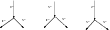
Refer to caption
Figure 3:

The nonzero components of π\pi

The computation of [π,υ][\pi,\upsilon] consists in gluing the graphs of the two vector fields υ,π\upsilon,\pi and searching for non-zero graphs. This gives, that [π,υ]=π∘υ+υ∘π[\pi,\upsilon]=\pi\circ\upsilon+\upsilon\circ\pi corresponds to the graph in Fig. 4.

Refer to caption
Figure 4:

At the left, the vector field υ\upsilon and at the right the bracket [π,υ][\pi,\upsilon].

Thus, πt=π+t⁡[π,υ]\pi_{t}=\pi+t[\pi,\upsilon] and according with what is just said, πt\pi_{t} can be expressed in graph terms. Next, one checks the graphs in the expression of the operator D​Uπt​(υ)DU_{\pi_{t}}(\upsilon). In general, the graph corresponding to this operator, will receive a colored (∈𝔥∗)(\in\mathfrak{h}^{\ast}) edge from the horizontal axis, which goes either to a vertex of the graph or leaves to infinity. In the first case, there still has to be a colored edge leaving to infinity, which narrows down the open possibilities for graphs.

Refer to caption
Figure 5:

At the left, how the operator D​UπtDU_{\pi_{t}} looks like and at the right two a priori nonzero graphs.

In our example, and after the graphs appearing in π\pi, the ground edge leaves to infinity, so we search for contributions among the different types of graphs listed in 𝓍​ 5.5.1\mathcal{x}\;5.5.1 of [9] and which we recall in Fig. 6.

Refer to caption
Figure 6:

Possible graphs for D​UπtDU_{\pi_{t}}.

Using among others the argument that UU isn’t in the derived algebra [𝔤,𝔤][\mathfrak{g},\mathfrak{g}] of 𝔤\mathfrak{g}, we are left with two nonzero graphs for D​UπtDU_{\pi_{t}}, and after calculating their weights (equal to 112\frac{1}{12}),

DUπt(υ)=112(1l⁡(Z)∂U3−t​Zl​(Z)2∂U3).DU_{\pi_{t}}(\upsilon)=\frac{1}{12}\left(\frac{1}{l(Z)}\partial_{U}^{3}-\frac{tZ}{l(Z)^{2}}\partial_{U}^{3}\right). (33)

As a special but simple case, the graph in Fig. 7

Refer to caption
Figure 7:

Another zero contribution.

is also zero because when we’ll later evaluate at l∈{ξ/ξ|𝔥=λ|𝔥}l\in\{\xi\;/\;\xi|_{\mathfrak{h}}=\lambda|_{\mathfrak{h}}\} we’ll get l⁡(X)=0l(X)=0 from υ=−Xl⁡(Z)∂U,λ=E∗\upsilon=-\frac{X}{l(Z)}\partial_{U},\;\lambda=E^{\ast}. Graphically, the operator D​UπtDU_{\pi_{t}} is given by the sum at Fig. 8.

Refer to caption
Figure 8:

The solution graphically.

D​UπtDU_{\pi_{t}} is a commuting family of operators and so the solution of equation (32) is

e∫tD​Uπt​𝑑t.e^{\int_{t}DU_{\pi_{t}}dt}. (34)

As far as it concerns relations between (H(ϵ)0(𝔥λ⊥,d𝔥λ⊥,𝔮(ϵ)),∗M)≃(H(ϵ)0(𝔥λ⊥,d𝔥λ⊥,𝔮l(ϵ)),∗Ml)(H^{0}_{(\epsilon)}(\mathfrak{h}_{\lambda}^{\bot},d^{(\epsilon)}_{\mathfrak{h}_{\lambda}^{\bot},\mathfrak{q}}),\ast_{M})\simeq(H^{0}_{(\epsilon)}(\mathfrak{h}_{\lambda}^{\bot},d^{(\epsilon)}_{\mathfrak{h}_{\lambda}^{\bot},\mathfrak{q}_{l}}),\ast_{M_{l}}) and (Uℂ​(𝔤)/Uℂ​(𝔤)​𝔥λ)𝔥(U_{\mathbb{C}}(\mathfrak{g})/U_{\mathbb{C}}(\mathfrak{g})\mathfrak{h}_{\lambda})^{\mathfrak{h}} we can write

β−1((2UZ−V2)3−2Z2)=A¯∗MA¯∗MA¯=A¯3−2Z2,\beta^{-1}((2UZ-V^{2})^{3}-2Z^{2})=\bar{A}\ast_{M}\bar{A}\ast_{M}\bar{A}=\bar{A}^{3}-2Z^{2},\;\; (35)
β𝔮l−1​((2​U​Z−V2)3−2​Z2)=(2​U​Z−V2)3−2​Z2+4​Z3l⁡(Z)−2​Z4l​(Z)2.\beta_{\mathfrak{q}_{l}}^{-1}((2UZ-V^{2})^{3}-2Z^{2})=(2UZ-V^{2})^{3}-2Z^{2}+\frac{4Z^{3}}{l(Z)}-\frac{2Z^{4}}{l(Z)^{2}}. (36)

Indeed, for t=1t=1,

B𝔮,𝔮l((2UZ−V2)3−2Z2)=e[112​l​(Z)(1−Z2​l​(Z))∂U3]((2UZ−V2)3−2Z2)=B_{\mathfrak{q},\mathfrak{q}_{l}}((2UZ-V^{2})^{3}-2Z^{2})=e^{[\frac{1}{12l(Z)}(1-\frac{Z}{2l(Z)})\partial_{U}^{3}]}((2UZ-V^{2})^{3}-2Z^{2})=
((2​U​Z−V2)3− 2​Z2)+4​Z3l⁡(Z)−2​Z4l​(Z)2.((2UZ-\penalty\ V^{2})^{3}-\penalty\ 2Z^{2})+\penalty\ \frac{4Z^{3}}{l(Z)}-\penalty\ \frac{2Z^{4}}{l(Z)^{2}}.

Thus a first formula that one can derive is

β𝔮l−1(A)=e[112​l​(Z)(1−Z2​l​(Z))∂U3]β𝔮−1(A).\beta_{\mathfrak{q}_{l}}^{-1}(A)=e^{[\frac{1}{12l(Z)}(1-\frac{Z}{2l(Z)})\partial_{U}^{3}]}\beta_{\mathfrak{q}}^{-1}(A). (37)

So after evaluation at ll, we get

β𝔮l−1​(A3)​(l)=A¯3​(l),\beta_{\mathfrak{q}_{l}}^{-1}(A^{3})(l)=\bar{A}^{3}(l), (38)

and β𝔮l−1​(A)​(l)=β𝔮−1​(A)​(l)\beta_{\mathfrak{q}_{l}}^{-1}(A)(l)=\beta_{\mathfrak{q}}^{-1}(A)(l) by (37). If ϕ⁡(A)\phi(A) is the polynomial associated to AA, this in turn implies that the map

(Uℂ(𝔤)/Uℂ(𝔤)𝔥λ)𝔥∋A↦[l↦ϕ(A)(l)=(e[112​l​(Z)(1−Z2​l​(Z))∂U3]β𝔮−1(A))(l)](U_{\mathbb{C}}(\mathfrak{g})/U_{\mathbb{C}}(\mathfrak{g})\mathfrak{h}_{\lambda})^{\mathfrak{h}}\ni A\mapsto\left[l\mapsto\phi(A)(l)=\left(e^{[\frac{1}{12l(Z)}(1-\frac{Z}{2l(Z)})\partial_{U}^{3}]}\beta_{\mathfrak{q}}^{-1}(A)\right)(l)\right]

is polynomial. Let B¯=P⁡(A¯,Z¯),B=P⁡(Z,A)\bar{B}=P(\bar{A},\bar{Z}),B=P(Z,A) be two polynomial expressions in Sℂ​(𝔮)𝔥S_{\mathbb{C}}(\mathfrak{q})^{\mathfrak{h}} and (Uℂ​(𝔤)/Uℂ​(𝔤)​𝔥λ)𝔥(U_{\mathbb{C}}(\mathfrak{g})/U_{\mathbb{C}}(\mathfrak{g})\mathfrak{h}_{\lambda})^{\mathfrak{h}} respectively. We will omit the bar for ZZ in B¯\bar{B} as no confusion arises. Since we have verified the isomorphism on the generators A,ZA,Z 33 3 We didn’t actually verify it for Z but this is trivial as it is a central element. one can write

β𝔮−1(B)=e−124​Z∂U3B¯,\beta_{\mathfrak{q}}^{-1}(B)=e^{-\frac{1}{24Z}\partial_{U}^{3}}\bar{B}, (39)

where β𝔮l−1​(B)=B¯=P⁡(A¯,Z)\beta_{\mathfrak{q}_{l}}^{-1}(B)=\bar{B}=P(\bar{A},Z). The numerator of the exponential here is justified by the fact that we haven’t yet evaluated at ll so by (37), 112​Z​(1−Z2​Z)=124​Z\frac{1}{12Z}(1-\frac{Z}{2Z})=\frac{1}{24Z}. An easy calculation with equation (39) verifies that β𝔮−1​(A3)=A¯3−2​Z2\beta_{\mathfrak{q}}^{-1}(A^{3})=\bar{A}^{3}-2Z^{2} as calculated by means of the Moyal product in (28). So the final formula we get is

β𝔮−1(B)(l)=e−124​l​(Z)∂U3B¯(l).\beta_{\mathfrak{q}}^{-1}(B)(l)=e^{-\frac{1}{24l(Z)}\partial_{U}^{3}}\bar{B}(l).

As a conclusion, we see that under (25), the map β𝔮l\beta_{\mathfrak{q}_{l}} becomes an isomorphism when evaluated on l∈λ+𝔥⊥l\in\lambda+\mathfrak{h}^{\bot} constructing a character of (Uℂ​(𝔤)/Uℂ​(𝔤)​𝔥λ)𝔥(U_{\mathbb{C}}(\mathfrak{g})/U_{\mathbb{C}}(\mathfrak{g})\mathfrak{h}_{\lambda})^{\mathfrak{h}}.

This way we verify and generalize the result of [1]. There the authors prove the isomorphism (U⁡(𝔤)/U⁡(𝔤)​𝔥)𝔥≃(S⁡(𝔤)/S⁡(𝔤)​𝔥)𝔥(U(\mathfrak{g})/U(\mathfrak{g})\mathfrak{h})^{\mathfrak{h}}\simeq(S(\mathfrak{g})/S(\mathfrak{g})\mathfrak{h})^{\mathfrak{h}} in the case where exists a common polarization for all elements ll. In that case, there is an obvious choise of supplementary 𝔮l\mathfrak{q}_{l} suggested by the condition (25). We generalized this result, by showing that whenever there isn’t such a convenient polarization, in order to construct a character one has to choose 𝔮l\mathfrak{q}_{l} transversally with respect to 𝔟l,𝔥\mathfrak{b}_{l},\mathfrak{h} and then evaluate β𝔮l\beta_{\mathfrak{q}_{l}} on ll.

On the other hand, these methods permit us to compute explicitly the pseudodifferential operator appearing in the character formula and composed with β𝔮−1\beta_{\mathfrak{q}}^{-1}. This way we can write down the formula of the character, a task almost impossible otherwise.

Theorem 3.1

Let 𝔤\mathfrak{g} be the real nilpotent Lie algebra, generated by the elements X,U,V,E,Z{X,U,V,E,Z}, with non-trivial brackets [U,V]=E,[X,U]=V,[X,V]=Z.[U,V]=E,[X,U]=V,[X,V]=Z. Let λ=E∗∈𝔤∗\lambda=E^{\ast}\in\mathfrak{g}^{\ast}, and consider the Lie subalgebra 𝔥=ℝ​X⊕ℝ​E\mathfrak{h}=\mathbb{R}X\oplus\mathbb{R}E of 𝔤\mathfrak{g}. For 𝔮=<Z,V,U>\mathfrak{q}=<Z,V,U> and 𝔮l=<Z,V,X−l⁡(Z)​U+l⁡(V)​V>\mathfrak{q}_{l}=<Z,V,X-l(Z)U+l(V)V> with l⁡(Z)≠0l(Z)\neq 0, we have that for u∈(U⁡(𝔤)/U⁡(𝔤)​𝔥λ)𝔥u\in(U(\mathfrak{g})/U(\mathfrak{g})\mathfrak{h}_{\lambda})^{\mathfrak{h}},

β𝔮l−1(u)=e[112​l​(Z)(1−Z2​l​(Z))∂U3]β𝔮−1(u),\beta_{\mathfrak{q}_{l}}^{-1}(u)=e^{[\frac{1}{12l(Z)}(1-\frac{Z}{2l(Z)})\partial_{U}^{3}]}\beta_{\mathfrak{q}}^{-1}(u), (40)

and if vv is a polynomial in (U⁡(𝔤)/U⁡(𝔤)​𝔥λ)𝔥(U(\mathfrak{g})/U(\mathfrak{g})\mathfrak{h}_{\lambda})^{\mathfrak{h}} then β𝔮−1(v)(l)=e−124​l​(Z)∂U3β𝔮l−1(v)(l)\beta_{\mathfrak{q}}^{-1}(v)(l)=e^{-\frac{1}{24l(Z)}\partial_{U}^{3}}\beta^{-1}_{\mathfrak{q}_{l}}(v)(l).

The map

γC​T:v↦(e[112​l​(Z)(1−Z2​l​(Z))∂U3]β𝔮−1(v))(l)\gamma_{CT}:\;v\mapsto\left(e^{[\frac{1}{12l(Z)}(1-\frac{Z}{2l(Z)})\partial_{U}^{3}]}\beta_{\mathfrak{q}}^{-1}(v)\right)(l)

is a character of (U⁡(𝔤)/U⁡(𝔤)​𝔥λ)𝔥(U(\mathfrak{g})/U(\mathfrak{g})\mathfrak{h}_{\lambda})^{\mathfrak{h}}.

Acknowledgements. This paper is the sequence of [3] and also comes out from the PhD thesis [2]. The author would like to gratefully thank Charles Torossian for his inspiring guidance and supervision during these years. He would also like to thank Simone Gutt and Fred Van Oystaeyen for their kind hospitality.

References

  • [1] A. Baklouti, J. Ludwig Invariant Differential Operators on Certain Nilpotent Homogeneous spaces Monatsh. Math. (134) (2001)
  • [2] P. Batakidis Deformation Quantization and Lie theory, 174 pp., These de Doctorat, Universite Paris 7, 2009.
  • [3] P. Batakidis On the isomorphism between the reduction algebra and the invariant differential operators on Lie groups. Submitted, Preprint (2010)
  • [4] Y. Benoist Analyse Harmonique sur les espaces Symetriques nilpotents. J. of Funct. Anal. 59, 211-254, (1984)
  • [5] P. Bernat, N. Conze, M. Duflo, M. Levy-Nahas, M. Rais, P. Renouard, M. Vergne Representations des groupes de Lie resolubles. Monographies de la Societe Mathematique de France, No. 4. Dunod, Paris, (1972).
  • [6] A.S. Cattaneo, G. Felder Coisotropic submanifolds in Poisson geometry and branes in the Poisson Sigma model. Lett.Math.Phys. 69 (2004) 157-175
  • [7] A.S. Cattaneo, G. Felder Relative formality Theorem and quantization of coisotropic submanifolds., Adv. Math. 208, (2007), no. 2, 521-548
  • [8] A.S. Cattaneo, B. Keller, Ch. Torossian, A. Bruguieres. Deformation, quantization, theorie de Lie. Collection Panoramas et Synthese n 20, SMF 2005.
  • [9] A.S. Cattaneo, Ch. Torossian, Quantification pour les paires symmetriques et diagrames de Kontsevich. Annales Sci. de l’Ecole Norm. Sup. (5) 2008, 787–852.
  • [10] L.J. Corwin, F.P. Greenleaf Representations of nilpotent Lie groups and their applications. Cambridge University Press, (1990)
  • [11] L.J. Corwin, F. P. Greenleaf Commutativity of invariant differential operators on nilpotent homogeneous spaces with finite multiplicity. Comm. Pure Appl. Math. 45 (1992), no. 6, 681–748.
  • [12] L.J. Corwin, F.P. Greenleaf Spectral decomposition of invariant differential operators on certain nilpotent homogeneous spaces. J. Funct. Anal. 108 (1992), no. 2, 374–426.
  • [13] J. Dixmier Algebres enveloppantes. Les Grands Classiques Gauthier-Villars. Editions Jacques Gabay, Paris, (1996).
  • [14] H. Fujiwara Representations monomiales des groupes de Lie nilpotents. Pacific J. of Mathematics, 127 (1987), no. 2, 329–352.
  • [15] H. Fujiwara Analyse harmonique pour certaines representations induites d’un groupe de Lie nilpotent. J. Math. Soc. Japan 50 (1998), no. 3, 753–766.
  • [16] H. Fujiwara Correction to: “Harmonic analysis for certain induced representations of a nilpotent Lie group” [J. Math. Soc. Japan 50 (1998), no. 3, 753–766] J. Math. Soc. Japan 52 (2000), no. 2, 483
  • [17] H.Fujiwara, G. Lion, B, Magneron, and S. Mehdi A commutativity criterion for certain algebras of invariant differential operators on nilpotent homogeneous spaces. Math. Ann. 327 (2003), no. 3, 513–544.
  • [18] M. Kontsevich Deformation quantization of Poisson manifolds. Lett. Math.Phys. 66 (2003), no. 3, 157–216.
  • [19] T. Koornwinder Invariant differential operators on nonreductive homogeneous spaces. math.RT/0008116, 11 pages (preprint 1981, not published).