Large-$\theta_{13}$ Perturbation Theory of Neutrino Oscillation for Long-Baseline Experiments

One of the most important progresses in particle physics in the last decades is the discovery of neutrino masses [1] and the lepton flavor mixing [2]. It was done through observing neutrino oscillation phenomena and it constitutes, up until this moment, only available experimental method for measuring lepton mixing parameters. $\Delta m^{2}_{32}$ and $\theta_{23}$ are determined by atmospheric neutrino observation by Super-Kamiokande [3, 4, 5], and then by accelerator neutrino experiments [6, 7]. $\Delta m^{2}_{21}$ and $\theta_{12}$ are measured independently by two types of experiments, the KamLAND reactor experiment [8, 9, 10] and the solar neutrino observation using various experimental techniques. For the latest results and for a review of the solar neutrino experiments see e.g., [11, 12] and [13], respectively. The remaining mixing angle $\theta_{13}$ is being explored by the ongoing and the upcoming accelerator [14, 15] and reactor neutrino experiments [16, 17, 18]. If it turned out that $\theta_{13}$ is not too small, we may proceed to measure CP violation by the lepton Kobayashi-Maskawa (KM) [19] phase $\delta_{\ell}$, to which we refer just $\delta$ in this paper.

It is expected that precision measurement is required to determine $\delta$ because CP violation effect is tiny due to suppression by the two small factors, $\Delta m^{2}_{21}/\Delta m^{2}_{31}$ and the Jarlskog coefficient $J\equiv c_{12}s_{12}c_{23}s_{23}c^{2}_{13}s_{13}$ [20]. Therefore, understanding of full complexity of neutrino oscillation phenomena would be of some help e.g., to design future experiments. An example of such is the parameter degeneracy [21, 22, 23], the problem of multiple copy of the solutions of mixing parameters allowed by given sufficient but limited numbers of experimental data. See [24] for a comprehensive overview of this phenomenon. To facilitate understanding of qualitative features of the neutrino oscillation, it is crucially important to have analytic formula, albeit approximate, for the oscillation probability. For relatively short baseline experiments, such as low-energy superbeam [25, 26, 27], the matter perturbation theory works [28, 29]. So far, most of the analyses for long baseline of $L\raise 1.29167pt\hbox{$\;>$\kern-7.5pt\raise-4.73611pt\hbox{$\sim\;$}}1000$ km were done by using the well known Cervera et al. formula [30].¹¹ 1 However, it was shown that analysis of the parameter degeneracy with the matter-perturbative formula has been proved to give a transparent view of the phenomenon [31, 32, 33], such as the decoupling between the degeneracies.

A simple way of deriving the Cervera et al. formula is to expand the exact oscillation probability by small expansion parameters, $\epsilon\equiv\Delta m^{2}_{21}/\Delta m^{2}_{31}$ and $s_{13}\equiv\sin\theta_{13}$, both to second order. While the former is known to be small $\epsilon\simeq 0.03$, the latter can be larger by almost an order of magnitude; Currently, it is only bounded from above by the Chooz limit, $s_{13}\raise 1.29167pt\hbox{$\;<$\kern-7.5pt\raise-4.73611pt\hbox{$\sim\;$}}0.18$ [34, 35, 36, 37]. We note that there is an indication for nonzero $\theta_{13}$ comparable to the Chooz limit from global fit of the solar, reactor, atmospheric, and the accelerator experiments [38, 39, 40, 41, 10, 12, 42]. Though the statistical significance of the indication is not high enough to be compelling, it certainly gives a good motivation for examining effects of such large values of $\theta_{13}$. Recently, a candidate event for $\nu_{e}$ appearance has been seen in the T2K experiment [43] which further strengthens the motivation for taking the large-$\theta_{13}$ hypothesis seriously.

If $\theta_{13}$ is large, higher order terms of $s_{13}$ would be needed to achieve better agreement with the exact oscillation probability. In this paper, we compute such higher order corrections of $s_{13}$. To facilitate systematic computation we formulate a perturbative framework by assuming $s_{13}$ as large as $\simeq\sqrt{\epsilon}$, which is comparable to the Chooz limit, and by taking the case of long enough baseline where the matter effect is comparable to the vacuum one. We call this framework as the “$\sqrt{\epsilon}$ perturbation theory” as opposed to the $\epsilon$ perturbation theory for the Cervera et al. formula as named in [33]. We derive the second order formulas for the oscillation probabilities in all channels. By taking the ansatz, $s_{13}\simeq\sqrt{\epsilon}$, our formulas will be valid for a wide range of $\theta_{13}$, $\epsilon\raise 1.29167pt\hbox{$\;<$\kern-7.5pt\raise-4.73611pt\hbox{$\sim\;$}}s_{13}\raise 1.29167pt\hbox{$\;<$\kern-7.5pt\raise-4.73611pt\hbox{$\sim\;$}}\sqrt{\epsilon}$. The $\sqrt{\epsilon}$ perturbation theory has been formulated earlier for relatively short baseline setting [44].

Some characteristic features of the computed formulas prompted us to think about general property of the oscillation probability, which resulted in the two general theorems described in Sec. II. For example, we show that the $\delta$ dependent terms in the $\nu_{e}$-related oscillation probabilities exist only in odd terms of $s_{13}$, and conversely, all the terms odd in $s_{13}$ have $\delta$ dependence. Thanks to the theorems, quite (un)interestingly, we can prove on general ground that the correction terms to the Cervera et al. formula have to be second order in $\epsilon$, eliminating the possibility of having large corrections. Yet, we will observe that at super long baseline, $L=4000$ km, our correction terms nicely fill a sizable gap between the exact oscillation probability and the Cervera et al. formula, which exists in a limited range of energy for $\theta_{13}$ comparable to the Chooz limit.

The possible large value of $\theta_{13}$ could generate some interesting effects. For example, there arise terms of order $\epsilon^{5/2}$ consisting solely of $\delta$-dependent terms in the $\nu_{e}$ appearance oscillation probability, which is smaller only by a factor of $\simeq 5$ compared to the existing terms in the Cervera et al. formula. Another intriguing feature arises when the non-standard interactions (NSI) of neutrinos are included into the system. For an extensive list of the references for NSI including the original ones see, e.g., [45]. Some of the NSI dependent terms get enhanced by large $\theta_{13}$, and decoupling of some NSI elements from the $\nu_{e}$-related appearance probabilities no more hold. On the other hand, the smallness of the correction terms to the Cervera et al. formula has a consequence that, quite naturally, their influence to parameter determination including the issue of parameter degeneracy is quite limited.

Following the discussion of general property of oscillation probability in Sec. II, we formulate our $\sqrt{\epsilon}$ perturbation theory (Sec. III), and derive the expressions of the oscillation probabilities valid to order $\epsilon^{2}$ in $\nu_{e}\rightarrow\nu_{\mu}$ and $\nu_{\mu}\rightarrow\nu_{\mu}$ channels (Sec. IV). The characteristic features of the formulas are shown to be understood thanks to the theorems given in Sec. II. The accuracy of our formula is checked against the exact results for a large value of $\theta_{13}$ (Sec. V). Then, we calculate order $\epsilon^{5/2}$ terms of the oscillation probability in the $\nu_{e}\rightarrow\nu_{\mu}$ channel which could be relevant for measurement of $\delta$ in its extreme precision (Sec. VI). Implications of smallness of the large $\theta_{13}$ corrections are explored by treating the parameter degeneracy (Sec. VII). The second-order formula of the oscillation probability in the $\nu_{e}$-related appearance channels is derived for systems with NSI (Sec. VIII). Concluding remarks are given in Sec. IX. Appendices are devoted for a proof of a general theorem for suppression of CP phase effect (Appendix A), the explicit expressions of the $S$ matrix elements in the $\theta_{23}$-rotated basis (Appendix B), and explicit forms of the oscillation probabilities in the remaining channels (Appendix C).

Before constructing perturbative framework of neutrino oscillation, let us discuss some generic features of the oscillation probability. They are interesting by themselves, and statements about $\cos\delta$ dependence do not appear to be explicitly spelled out in the literature to our knowledge. It will also help us to understand characteristic features of the perturbation theory of neutrino oscillation to be discussed in the rest of this paper. An example of this is that CP phase effect appear only in terms of half-integral order of the small expansion parameter $\epsilon$ in our $\sqrt{\epsilon}$ perturbation theory.

We note that the general features of neutrino oscillation probability which exactly hold with [46, 47] or without [48] constant matter density approximation can be used to prove some useful properties of the oscillation probabilities. That is, we call the readers’ attention to the following two theorems:

• •

  Theorem A: In $\nu_{e}$-related oscillation probabilities the $\delta$-dependence exists only in odd terms in $s_{13}$. Conversely, all the odd terms in $s_{13}$ are accompanied with either $\cos\delta$ or $\sin\delta$.

• •

  Theorem B: $\delta$-dependent terms in the oscillation probability in matter, not only $\sin\delta$ but also $\cos\delta$ terms, must come with the two suppression factors, $\frac{\Delta m^{2}_{21}}{\Delta m^{2}_{31}}$ and the reduced (or “not quite”) Jarlskog coefficient $J_{r}\equiv c_{12}s_{12}c_{23}s_{23}s_{13}$.

To prove the theorem A we note that $s_{13}$ and $\delta$ enter into the Hamiltonian through the single variable $z\equiv s_{13}e^{i\delta}$. Therefore, the oscillation probability $P$ can be written as a power series expansion as $P=\sum_{n,m}^{\infty}f_{nm}z^{n}(z^{*})^{m}$, where $f_{nm}=f^{*}_{mn}$ for reality of $P$. On the other hand, the result obtained in [48] by extending discussions in [49] says that there are only $\cos\delta$ and $\sin\delta$ terms in $\nu_{e}$ related oscillation probabilities, and no higher harmonics of $\delta$. It means that only the terms that satisfy $m=n\pm 1$ survive. It leaves the unique form of the oscillation probability $P=K(s^{2}_{13})s_{13}\cos\delta+M(s^{2}_{13})s_{13}\sin\delta$, where $K$ and $M$ are some functions. At the same time, this construction guarantees that all the odd terms in $s_{13}$ are accompanied by $\delta$. This is nothing but the theorem A.

Now, let us discuss the theorem B. If the adiabaticity holds existence of the suppression factors by the $\Delta m^{2}$ ratio and the angle factors for $\sin\delta$ terms is well known. In fact, one can show that the latter is precisely the Jarlskog coefficient $J\equiv c_{12}s_{12}c_{23}s_{23}c^{2}_{13}s_{13}$ thanks to the Naumov identity [50, 51]

where the quantities with over-bar in the left-hand side denote the ones in matter which correspond to the one in vacuum in the right-hand side of (1). Notice that $\cos\bar{\delta}$ does not contain $\sin\delta$ [47], and the proportionality between $\sin\bar{\delta}$ and $\sin\delta$ is also guaranteed by the Toshev identity $\bar{c}_{23}\bar{s}_{23}\sin\bar{\delta}=c_{23}s_{23}\sin\delta$ [52]. The equation (1) indicates that the $\sin\delta$ term vanishes in the limit of one of $\Delta m^{2}_{ij}\rightarrow 0$, or vanishing limit of one of the mixing angles.

Whether the same statement apply to $\cos\delta$ terms or not, or if the theorem B is valid at all for cases with generic matter density profiles, is not obvious. Apparently no general statement has been made in the literature. Vanishing of any $\delta$ dependence (including cosine) in the absence of $\Delta m^{2}_{21}$ can be proved similarly as the phase reduction theorem given in [33] as a special case of turning off the non-standard interactions. For constant matter density proportionality of $\cos\delta$ terms to the Jarlskog coefficient $J$ (reduced coefficient $J_{r}$) in the $\nu_{e}$-related channels (oscillation channels in the $\nu_{\mu}-\nu_{\tau}$ sector) is explicitly proved in [47] by deriving the exact forms of the oscillation probabilities.²² 2 The difference of whether the suppression factor is provided by $J$ or $J_{r}$ does not make difference in our following discussions. Hence, we do not discuss this point further apart from making a brief comment in Appendix A. Therefore, what is left is to show that the last statement holds under arbitrary matter density profile without recourse to the assumption of adiabaticity. The proof for this general case is described in Appendix A.

In this section, we formulate a large-$\theta_{13}$ perturbation theory of neutrino oscillation. We use an ansatz

to formulate our perturbative framework, hence the name “$\sqrt{\epsilon}$ perturbation theory”. It implies $\sin^{2}2\theta_{13}\simeq 0.12$, the value comparable with the Chooz limit. We work in anticipation of long baselines of several thousand kilometers, so that $r_{A}\equiv a/\Delta m^{2}_{31}\sim\mathcal{O}(1)$, and $\Delta m^{2}_{31}L/E\sim\mathcal{O}(1)$ to be not far from the first oscillation maximum. Hereafter, $a\equiv 2\sqrt{2}G_{F}N_{e}(x)E$ is a coefficient for measuring the matter effect on neutrinos propagating in medium of electron number density $N_{e}(x)$ [53], where $G_{F}$ is the Fermi constant and $E$ is the neutrino energy. In perturbative calculation of the oscillation probability we take constant electron number density approximation.

If we take the ansatz $s_{13}\simeq\epsilon$ (which corresponds to $\sin^{2}2\theta_{13}\simeq 4\epsilon^{2}\simeq 4\times 10^{-3}$) instead of (2), we obtain the widely used Cervera et al. formula [30] by keeping terms to order $\epsilon^{2}$. Of course, there may exist the other small (or large) parameters, such as $\Delta m^{2}_{31}L/E$ and $a/\Delta m^{2}_{31}$ at short baselines, depending upon the experimental settings. The similar $\sqrt{\epsilon}$ perturbation theory for shorter baselines is discussed by assuming $r_{A}\sim\sqrt{\epsilon}$ [44].

The remaining potentially small parameters would be $\pi/4-\theta_{23}$, but we do not take it as an expansion parameter for two reasons:³³ 3 Nonetheless, one can of course further expand the oscillation probability in terms of $\pi/4-\theta_{23}$ assuming it small, as is done e.g., in [54, 55, 56]. (1) A rather large range is currently allowed for $\theta_{23}$, and moreover the situation will not be changed even with the next generation experiments [57]. (2) As will become evident in formulating our perturbative framework $\theta_{23}$ is an “external parameter” which is irrelevant in doing perturbative computation.

We follow [33] to formulate the perturbative treatment of neutrino oscillation. The $S$ matrix describes possible flavor changes after traversing a distance $L$,

and the oscillation probability is given by

When the neutrino evolution is governed by the Schrödinger equation, $i\frac{d}{dx}\nu=H\nu$, $S$ matrix is given as

where $T$ symbol indicates the “time ordering” (in fact “space ordering” here). The right-hand side of (5) may be written as $e^{-iHL}$ for the case of constant matter density. In the standard three-flavor neutrinos, Hamiltonian is given (with $a=2\sqrt{2}G_{F}N_{e}E$) by

where $\Delta m^{2}_{ji}\equiv m^{2}_{j}-m^{2}_{i}$. In (III) $U$ is the MNS matrix and can be written in the standard notation as

with the notation $s_{ij}\equiv\sin\theta_{ij}$ etc. and $\delta$ being the lepton KM phase.

To formulate perturbative treatment it is convenient to work with the tilde basis defined as $\tilde{\nu}_{\alpha}=(U_{23}^{\dagger})_{\alpha\beta}\nu_{\beta}$, in which the Hamiltonian is related to the flavor basis one as [58]

where $U_{23}$ is defined in (III). The $S$ matrix in the flavor basis is related to the $S$ matrix in the tilde basis as

where $\tilde{S}(L)=T\text{exp}\left[-i\int^{L}_{0}dx\tilde{H}(x)\right]$. The unperturbed part of the tilde-basis Hamiltonian is given by

where $\Delta\equiv\frac{\Delta m^{2}_{31}}{2E}$ and $r_{A}\equiv\frac{a}{\Delta m^{2}_{31}}$. While the perturbed part is written with another simplified notation $r_{\Delta}\equiv\frac{\Delta m^{2}_{21}}{\Delta m^{2}_{31}}$ as

The first, second, third, and the fourth terms in (III) are of order $\epsilon^{\frac{1}{2}}$, $\epsilon^{1}$, $\epsilon^{\frac{3}{2}}$, and $\epsilon^{2}$, respectively.

To calculate $\tilde{S}(L)$ perturbatively we define $\Omega(x)$ as $\Omega(x)=e^{i\tilde{H}_{0}x}\tilde{S}(x)$, which obeys the evolution equation

where

Then, $\Omega(x)$ can be computed perturbatively as

where the “space-ordered” form in (46) is essential because of the non-commutativity between $H_{1}$ of different locations. Having obtained $\Omega(x)$ $\tilde{S}$ matrix can be written as

The results of $\tilde{S}(x)$ matrix elements to second-order in $\epsilon$ are given in Appendix B. Then, the $S$ matrix can be computed by making a rotation in (2-3) space $S=U_{23}\tilde{S}U_{23}^{\dagger}$ as in (24). (See ().) Finally, the oscillation probability can readily be obtained by using (4). For example, the one in the $\nu_{e}\rightarrow\nu_{\mu}$ channel can be given by using the $\tilde{S}$ matrix elements as

In this section, we present perturbative expressions of the oscillation probabilities in the $\nu_{e}$ related and the $\nu_{\mu}-\nu_{\tau}$ sectors to order $\epsilon^{2}$ in our $\sqrt{\epsilon}$ perturbation theory. All the formulas in this section are given in the form as

in which we use $L$ to denote the baseline distance. Some order $\epsilon^{5/2}$ terms will be discussed in Sec. VI. The antineutrino probability can be obtained from the neutrino probability by the replacement as $P(\bar{\nu}_{\alpha}\rightarrow\bar{\nu}_{\beta};\delta,a)=P(\nu_{\alpha}\rightarrow\nu_{\beta};-\delta,-a)$. Similarly, the T-conjugate one is given by $P(\nu_{\beta}\rightarrow\nu_{\alpha};\delta,a)=P(\nu_{\alpha}\rightarrow\nu_{\beta};-\delta,a)$. Remember that the following abbreviated notations are used: $\Delta\equiv\frac{\Delta m^{2}_{31}}{2E}$, $r_{\Delta}\equiv\frac{\Delta m^{2}_{21}}{\Delta m^{2}_{31}}$, and $r_{A}\equiv\frac{a}{\Delta m^{2}_{31}}$.

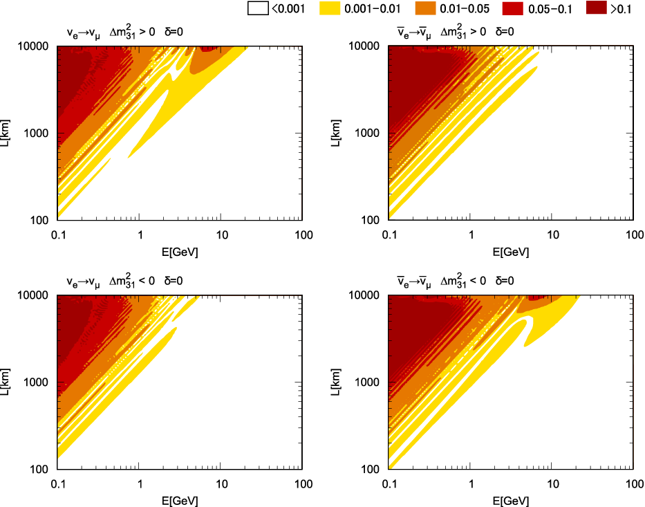
In this section, we examine numerical accuracy of our perturbative formulas of the oscillation probabilities computed to order $\epsilon^{2}$ for $\theta_{13}$ of the order of the Chooz limit. We focus on the $\nu_{e}\rightarrow\nu_{\mu}$ channel whereas we also did the similar analysis in the $\nu_{\mu}\rightarrow\nu_{\mu}$ channel [61]. To display accuracy of the approximate formula, two typical ways of plot are available, namely, the absolute difference $|P_{e\mu}^{\text{exact}}-P_{e\mu}^{\text{2nd}}|$, and the relative difference $|P_{e\mu}^{\text{exact}}-P_{e\mu}^{\text{2nd}}|/P_{e\mu}^{\text{exact}}$, where $P_{e\mu}^{\text{exact}}$ and $P_{e\mu}^{\text{2nd}}$ denote, respectively, numerically evaluated exact oscillation probability and our approximate formula to order $\epsilon^{2}$.

In Figs. 1 and 2, the absolute and the relative differences, respectively, are presented by using the color graduation plots in $E-L$ space. We note that the comparison between the Cervera et al. formula and the exact result was performed in [58]. We use the similar format to make easier the comparison between our and their results. A comparison between the relevant panels in Figs. 3 and 4 of [58] and Figs. 1 and 2 indicates that our large-$\theta_{13}$ correction terms improves the accuracy of the approximate formula in a wide region in $E-L$ space. It is even more so considering that our assumed value of $\sin\theta_{13}$ is about a factor of two larger than their largest value. The features of the plots with other values of $\delta$ are quite similar to those presented in Figs. 1 and 2, and hence we do not present them. For the same reason, only the case of normal mass hierarchy is shown in Fig. 2.

To see more clearly how good (or bad) are the approximations by our and the Cervera et al. formula, we present in Fig. 3 the oscillation probability as a function of neutrino energy calculated numerically (denoted as “exact”, green dashed line), computed by using the Cervera et al. formula (blue dash-dotted line), computed with our perturbative formula (red solid line). The left and the right panels in Fig. 3 are for baselines $L=1000$ km and $L=4000$ km, for which the matter density is taken as 2.8 g/cm³ and 3.6 g/cm³, respectively. The mass hierarchy is taken as the normal one, $\Delta m^{2}_{31}>0$. $\theta_{13}$ is taken as $\sin\theta_{13}=0.18$ which is close to the Chooz limit, and $\delta=0$. The values of the remaining mixing parameters used are given in the caption of Fig. 1.

As seen in Fig. 3, the difference between the exact and the Cervera et al. formula is very visible (modest) at $L=4000$ km ($L=1000$ km). It is notable that the higher order corrections of $s_{13}$ incorporated in our formula nicely fill the gap between them. To understand the nature of the gap we have examined the other cases of mass hierarchy and (anti-)neutrino channel. The features of the three curves presented in Fig. 3 are very similar to the ones of antineutrino channel with the inverted hierarchy, both $r_{A}\equiv\frac{a}{\Delta m^{2}_{31}}>0$. The features in the other two cases, antineutrino channel with the normal hierarchy and neutrino channel with the inverted hierarchy, both $r_{A}<0$, are similar to each other. They are not presented because the differences among the three curves are much smaller for both $L=1000$ km and 4000 km. We have checked that the features mentioned above are very similar for other values of $\delta$.

As was proved in Sec. IV.3 the higher order corrections (the non-Cervera terms) are of order $\epsilon^{2}\simeq 10^{-3}$, and hence the large gap between the exact and the Cervera et al. formula, in particular the one at $L=4000$ km, must arise as a result of some enhancement. It is caused by the factor $1/(1-r_{A})$, as seen from the relevant energies of the gap and the features of the other channels and hierarchies; It is nothing but the enhancement due to the MSW resonance [62, 63]. It is interesting that our formula, though perturbative, can incorporate the enhancement effect for baselines up to several thousand km for which $\Delta L\simeq 5$, not too far from $\sim\mathcal{O}(1)$. For baseline of order $L\sim 10000$ km the resonance enhancement becomes more significant and the difference between the exact and our formula (as well as the Cervera et al.’s) blows up. Of course, it is outside the region of validity of the perturbative treatment, and one need to sum up $1/(1-r_{A})$ effect. It is beyond the scope of this paper.

For large $\theta_{13}$ comparable to the Chooz limit, it may be meaningful to analyze the order $\epsilon^{5/2}$ terms, though it has an extra suppression of $\sqrt{\epsilon}\simeq 0.2$ compared to the order $\mathcal{O}\left(\epsilon^{2}\right)$ terms. It could be particularly relevant for the $\nu_{e}\rightarrow\nu_{\mu}$ channel for which an extreme accuracy may be reached e.g., by neutrino factory [64]. Our interest in the $\epsilon^{5/2}$ terms is primarily due to that they consist only of $\delta$-dependent terms, the property enforced by the theorem A. Fortunately, it is easy to compute the order $\epsilon^{5/2}$ terms in the oscillation probability by using the $\tilde{S}$ matrix elements to order $\epsilon^{2}$ listed in Appendix B.

The results of the order $\epsilon^{5/2}$ terms in $P(\nu_{e}\rightarrow\nu_{\mu})$ which is to be added to the $\epsilon^{1}$, $\epsilon^{3/2}$, and $\epsilon^{2}$ terms given in Sec. IV.1 reads:

$P_{e\tau}^{(5/2)}$ can be obtained from $P_{e\mu}^{(5/2)}$ by the transformation $c_{23}\rightarrow-s_{23}$ and $s_{23}\rightarrow c_{23}$.

The distinctive feature of order $\epsilon^{5/2}$ terms in (), as compared to $\epsilon^{3/2}$ terms in (51), is that there exist much more profound type of $\delta$ dependence, not only correlated (as argument of cosine function) with $\frac{\Delta L}{2}$ but also to $\frac{r_{A}\Delta L}{2}$ and $\frac{(1\pm r_{A})\Delta L}{2}$. If measurement is sufficiently accurate to resolve such correlations different from the vacuum type, it must merit to achieve higher sensitivity to detect CP violation and accurately measure $\delta$. However, quantitative analysis to examine this feature to reveal the required experimental conditions, such as which energy resolution and how many baselines are required etc. is beyond the scope of this paper.