Conformal Invariance, Dark Energy, and CMB Non-Gaussianity
Abstract
In addition to simple scale invariance, a universe dominated by dark energy naturally gives rise to correlation functions possessing full conformal invariance. This is due to the mathematical isomorphism between the conformal group of certain three dimensional slices of de Sitter space and the de Sitter isometry group . In the standard homogeneous, isotropic cosmological model in which primordial density perturbations are generated during a long vacuum energy dominated de Sitter phase, the embedding of flat spatial sections in de Sitter space induces a conformal invariant perturbation spectrum and definite prediction for the shape of the non-Gaussian CMB bispectrum. In the case in which the density fluctuations are generated instead on the de Sitter horizon, conformal invariance of the horizon embedding implies a different but also quite definite prediction for the angular correlations of CMB non-Gaussianity on the sky. Each of these forms for the bispectrum is intrinsic to the symmetries of de Sitter space, and in that sense, independent of specific model assumptions. Each is different from the predictions of single field slow roll inflation models, which rely on the breaking of de Sitter invariance. We propose a quantum origin for the CMB fluctuations in the scalar gravitational sector from the conformal anomaly that could give rise to these non-Gaussianities without a slow roll inflaton field, and argue that conformal invariance also leads to the expectation for the relation between the spectral indices of the scalar and tensor power spectrum. Confirmation of this prediction or detection of non-Gaussian correlations in the CMB of one of the bispectral shape functions predicted by conformal invariance can be used both to establish the physical origins of primordial density fluctuations, and distinguish between different dynamical models of cosmological vacuum dark energy.
I Introduction
The Cosmic Microwave Background (CMB) provides an essentially unique window on the universe at very great distances from our local neighborhood, or equivalently at very early times before the present epoch. The fact that the CMB exists at all, with a high degree of isotropy and a thermal spectrum, is evidence that the primordial universe was to high accuracy at some point in a nearly uniform state of thermal equilibrium, and therefore in causal contact at a time and place prior to the last scattering of the CMB photons. The small but measurable anisotropy in the CMB presents the most compelling clues to the possible quantum origin of the universe, as well as the source of the complex large scale structure of matter we observe today. Determining the statistical properties of CMB anisotropies, and in particular, non-Gaussian primordial correlations, offers the possibility of discriminating between different cosmological models of the very early and very distant universe [1, 2].
In parallel to the CMB measurements by COBE [3], WMAP [4] and the Planck satellite [5], the discovery of cosmological dark energy at the present epoch [6] emphasizes the need for a more fundamental understanding of vacuum energy and the cosmological ‘constant.’ A comprehensive theory of dark energy may have consequences also for the origin of the CMB anisotropy. In this paper we explore the possible relation between cosmological dark energy and CMB properties. In order to investigate this connection in a way which is as free as possible from dynamical assumptions, we follow an essentially kinematical approach, deriving the form of the non-Gaussian correlations of CMB anisotropies directly from the inherent symmetry group of a dark energy dominated de Sitter universe. In particular, we show that embedding the three dimensional surface on which the fluctuations giving rise to the CMB anisotropies originate in four dimensional de Sitter spacetime leads naturally to conformal invariance and determines the angular shape of the three-point CMB bispectrum, which is different for different embeddings, but otherwise independent of particular dynamical assumptions.
The standard cosmological model is based on the assumption of a globally spatially homogeneous and isotropic universe with uniform expansion. This is described by a Friedmann-Lemaître-Robertson-Walker (FLRW) line element with flat spatial sections,
| (1) |
in which the FLRW scale factor obeys the Einstein-Friedmann eq.,
| (2) |
in cosmological comoving time . The total energy density of the universe and pressure of the cosmological fluid are also assumed spatially homogeneous and isotropic on average at large scales and satisfy the covariant conservation eq. for a perfect fluid,
| (3) |
which assumes no entropy production or viscosity. In the FLRW cosmological model all that is left then to specify is the eq. of state relationship between and (with ) for the various components of the cosmological fluid at different epochs of the universe’s expansion. CMB anisotropies are treated as small () linear perturbations away from this exactly homogeneous and isotropic background, whose effect on the mean geometry is negligible and may be neglected at early times.
If at some epoch the energy density and pressure are dominated by a cosmological constant term , for which
| (4) |
is a constant, then it follows from (2) and (3) that the expansion rate is a also constant, and the scale factor,
| (5) |
describes an exponentially expanding phase. The line element (1) with (5) then is a particular coordinatization of de Sitter spacetime, the maximally symmetric solution of Einstein’s equations with a positive cosmological term.
This exponential inflationary de Sitter expansion takes regions that were in close causal contact initially and expands them to very great distances apart, potentially accounting for the thermal spectrum and high degree of isotropy observed in the CMB emitted from different directions in the sky. Primordial quantum fluctuations in this de Sitter inflationary epoch are held to be responsible for the observed small anisotropy in the CMB, and naturally gives rise to the approximately scale invariant CMB power spectrum consistent with the COBE and WMAP data [3, 4]. This agreement is one of the principal arguments in favor of inflationary models, broadly defined as the hypothesis that the universe passed through a de Sitter phase early in its history, during which an effective and nearly constant cosmological constant energy density dominated all other forms of energy, and the cosmological expansion was exponential according to (5) for at least several dozen -foldings [7].
Although this simple picture is quite appealing on general grounds, a fundamental theory for this exponential expansion, the physical origin of the effective cosmological constant term associated with the energy density of the ‘vacuum’ itself, its value today, and vacuum energy generally is lacking. In its place a number of different phenomenological models of inflation have been suggested [7]. The simplest of these models postulates a single scalar field (called the “inflaton”) which has a non-negative potential energy function . If and are nearly constant for a long enough period of time, acts as a nearly constant source in (2) which drives the exponential expansion (5) for many -foldings. Eventually the inflaton field is supposed to roll down its potential, preserving spatial homogeneity and isotropy in the large, and settle to a value with (or nearly zero) at the minimum of the potential. Although the mean value of the inflaton field is assumed to be spatially homogeneous and isotropic, small spatially inhomogeneous fluctuations in this field couple (linearly) to gravity. During the inflationary epoch these generate fluctuations in the metric geometry of space and the local gravitational potential that eventually induce corresponding spatiotemporal fluctuations in the local temperature of the cosmological fluid, in particular at the epoch of matter-radiation decoupling. In this picture these primordial fluctuations of quantum origin are imprinted on the radiation at the time of last scattering and lead to the small angular anisotropies observed in the CMB today [7, 8].
In this class of single field “slow roll” inflaton models the primordial CMB fluctuations have a (nearly) scale invariant Harrison-Zel’dovich spectrum [9] and obey (nearly) Gaussian statistics, with small corrections coming from the slow roll dynamics itself, which are probably too small to be observed even by Planck [10]. It follows that any detection of non-Gaussian three-point correlations on the microwave sky of primordial origin will immediately falsify the simplest single field slow roll inflation model, and provide an important observational constraint on the physical origins of the primordial fluctuations themselves.
Several years ago the present authors suggested that the approximate scale invariance of the CMB power spectrum might be a hint of a more general conformal invariance property of the primordial fluctuations, that doesn’t rely on any slow roll inflaton field(s) or similar specific dynamical models of inflation [11]. Since scale and conformal invariance arises in other branches of physics, such as turbulent flows and critical phenomena, with universal behavior independent of the particular dynamical details or short distance interactions of the system, the approximate scale invariance of the primordial CMB power spectrum may be connected to rather different and universal physics than the slow roll hypothesis assumes in the simplest models of inflation. We suggested that the conformal invariance hypothesis could be tested by detection of non-Gaussian statistics in the CMB and in particular, the measurement of the angular correlations in the three-point bispectrum. The generic assumption of conformal invariance fixes the form of the bispectrum without any reference to specialized models of inflation, provided only that a conformally invariant phase of the universe’s spacetime history existed during which the CMB fluctuations were generated. Although the overall magnitude of the CMB correlation functions cannot be determined by the conformal invariance hypothesis, and requires more specific dynamical information about the origin of the fluctuations, the shape of the non-Gaussian correlations is highly constrained by the essentially kinematic requirements of conformal symmetry alone, and hence can act as a powerful probe of a possible conformal phase of the universe.
In this paper we will take this idea one step further, demonstrating that full conformal invariance and conformal field theory (CFT) behavior is in fact a natural consequence of the isometries of de Sitter spacetime, which is generated by a period of vacuum cosmological dark energy dominance. Specifically the de Sitter group is isomorphic to the group of conformal transformations of certain three dimensional foliations (slicings) of de Sitter space. Moreover, the several mathematical possibilities of different slicings imply different realizations of conformal symmetry and determine different shapes of the CMB bispectrum, which can be distinguished observationally. Since these different realizations correspond to quite different physical origins of CMB anisotropies, and are related to the dominance of a de Sitter phase in different cosmological models of vacuum energy, there is the intriguing possibility of elucidating the physics of cosmological dark energy by future measurement of the angular form of CMB non-Gaussian correlations.
The first way that conformal invariance can arise is by a long period of vacuum energy dominance in the usual FLRW coordinates (1) with flat spatial sections. The limiting behavior of de Sitter invariant correlation functions in the asymptotic region , after many de Sitter -foldings, stretches all distance scales by the exponential expansion factor (5) and only the terms which fall off most slowly with distance survive. In this limit the correlation functions of any anisotropic density fluctuations exhibit conformal behavior [12]. This is the mathematical basis for one form of dS/CFT correspondence [13, 14, 15, 16], by which we mean conformal behavior of fields and Green’s functions in dimensional (bulk) de Sitter space at its dimensional boundary at spacelike infinity, c.f. Fig. 6. The late time limit of three dimensional spacelike sections of (1) embedded in four dimensional de Sitter spacetime leads to simple conformal behavior with a single conformal weight, and a specific form of the non-Gaussian bispectrum given by eqs. (48)-(51) below.
No particular dynamical mechanism of the origin of the fluctuations needs to be specified, and in that sense this prediction (48) of the bispectral shape is model independent, following from purely kinematic embedding of the conformal group of in the de Sitter group. It is necessary only that the fluctuations arose at a constant FLRW cosmic time late in the de Sitter expansion (so that any effects of non-de Sitter invariant initial conditions are suppressed), and that the fluctuations are intrinsic to de Sitter space, respecting all of its built-in symmetries. This is a quite different assumption than that made in current inflationary models based on slow roll out of de Sitter space, and as we discuss in detail in Sec. 3, eqs. (48)-(51) give a different form of the CMB angular bispectrum than that predicted in single field slow roll models. Thus any detection of the non-Gaussian CMB bispectrum and determination of its angular dependence (regardless of its overall amplitude) has the ability to distinguish between an intrinsic origin of the primordial fluctuations of the kind we discuss in this paper, and specific phenomenological dynamical models of their origin, such as that of the slow roll scenario or its variants.
Freeing the origin of primordial fluctuations from a particular class of models based on a (so far unobserved) scalar inflaton field also allows for quite different global cosmologies than strictly homogeneous, isotropic form (1). A second and quite distinct way that conformal invariance is mathematically realized in de Sitter spacetime is through the presence of a cosmological horizon. In inflationary models the primordial fluctuations leave the de Sitter horizon of the inflationary epoch and re-enter the cosmological Hubble sphere much later in the history of the universe. However no direct local observation of the CMB can exclude the possibility that the fluctuations arose on or near the cosmological horizon itself, and that the global geometry of the universe outside our cosmological horizon is quite different than that described by the FLRW line element (1). The fact that cosmological dark energy is some % of the energy density of the present universe is a powerful reminder of the lack of a basic understanding of vacuum energy, much less a complete theory of its dynamical role in cosmology. It is quite possible that a more fundamental understanding of vacuum dark energy will require a radical revision of the basic assumptions of cosmology in toto, including global spatial homogeneity and isotropy, and that the CMB anisotropies may have arisen in a quite different way from a nearly de Sitter invariant conformal phase possibly related with the presence of cosmological dark energy at more recent epochs.
In this paper we shall also describe an alternate embedding of the conformal group of directions in the sky (the celestial sphere ), appropriate if the fluctuations are generated near the de Sitter cosmological horizon itself, rather than on fixed sections. In this case the bulk space is the three dimensional space of constant static time in (79), and is its two dimensional horizon boundary. This slicing leads to yet a third, non-Gaussian bispectral form (106), different than either that determined by a slow roll model or conformal invariance considerations based on (1) and . If the third form of the non-Gaussian bispectrum is observed in the CMB, it will lead to quite different cosmological consequences, possibly related to a more fundamental understanding of the spacetime dependent dynamics of vacuum energy associated with the cosmological horizon, and the residual cosmological dark energy observed in the present epoch. Thus the observation of a non-Gaussian bispectrum by WMAP or Planck of a definite angular form has the potential to distinguish between quite different global geometries of the universe and quite different loci and physical mechanisms for the origin of CMB anisotropies, both testing the homogeneity and isotropy hypothesis of the standard FLRW cosmology, and potentially leading to dynamical models for cosmological dark energy on the largest scales.
The paper is organized as follows. In the next section we review the basic kinematics and isometries of de Sitter space, and the isomorphism between generators of the de Sitter isometries and the conformal transformations of , which is the mathematical basis for dS/CFT correspondence. In Section III we derive the conformal Ward identities that follow from this correspondence and use them to determine the form of the three-point non-Gaussian bispectrum for scalar fluctuations at a fixed FLRW time . In Section IV we give the general solution for the gauge invariant gravitational potentials of the linearized Einstein eqs. around de Sitter space in terms of the stress energy tensor perturbations, necessary to connect the density perturbations to the observable CMB anisotropies. In Section V we consider the static time slicing of de Sitter space and the induced conformal invariance of correlation functions on the cosmological horizon. The conformal Ward identities of the spherical horizon lead to a completely different form again of the non-Gaussian bispectrum in angular coordinates on the sky. In Sec. VII we discuss a possible origin for this non-Gaussian conformal correlation functions from the fluctuations of the cosmological horizon modes derived from the trace anomaly of any massless quantum matter fields in curved space, and show that they can give rise to the scale invariant Harrison-Zel’dovich power spectrum. In Sec. VIII we extend these considerations of conformal invariance to the spectrum of transverse, traceless spin- fields, i.e. gravitational waves, which will influence CMB polarization measurements. We conclude in Sec. IX with a summary of our main results and a discussion of the possibility of detection of CMB non-Gaussianities becoming a discriminating probe of the physics of dark energy and the large scale geometry of the universe.
For the convenience of the reader we have collected in the seven Appendices a number of known and some less well known mathematical properties of de Sitter spacetime used in the text. These are (A) Geometry, Coordinates and dS/CFT Correspondence of de Sitter Space; (B) Killing Vectors of de Sitter Space in Flat FLRW and (C) Static Coordinates; (D) Invariant Distance and Correlation Functions; (E) The Conformal Group on ; (F) Exact Formulae for the Bispectral Shape Function (50); and (G) Differential Operators in de Sitter Space. Some of these results have been reported previously in Refs. [11, 14, 17, 18].
II Conformal Invariance of Flat Spatial Sections in de Sitter Space
The essential kinematical feature of a vacuum dark energy dominated de Sitter universe is that the conformal group of certain embeddings of three dimensional hypersurfaces in de Sitter spacetime may be mapped (either one-to-one or multiple-to-one) to the geometric isometry group of the full four dimensional spacetime into which the hypersurfaces are embedded [19]. The first example of such an embedding is that of flat Euclidean in de Sitter spacetime in coordinates (1). The conformal group of the three dimensional spatial sections is in fact identical (isomorphic) to the isometry group of the four dimensional de Sitter spacetime, as we now review.
Since (eternal) de Sitter space is maximally symmetric, it posseses the maximum number of isometries for a spacetime in dimensions, namely , corresponding to the solutions of the Killing equation,
| (6) |
Each of the linearly independent solutions to this eq. (labelled by ) is a vector field in de Sitter space corresponding to an infinitesimal coordinate transformation, that leaves the de Sitter geometry and line element (1) with (5) invariant. These are the generators of the de Sitter isometry group, the non-compact Lie group . The geometry and frequently used coordinates of de Sitter space are reviewed in Appendix A.
The isomorphism with conformal transformations of is that each of these solutions of (6) may be placed in one-to-one correspondence with the solutions of the conformal Killing eq. of three dimensional flat space , i.e.
| (7) |
In (6) the spacetime indices range over values and is the covariant derivative with respect to the full dimensional metric of de Sitter spacetime, whereas in (7), are dimensional spatial indices of the three Cartesian coordinates of Euclidean of one dimension lower with flat metric . Solutions to the conformal Killing eq. (7) are transformations of which preserve angles in . This isomorphism between geometric isometries of dimensional de Sitter spacetime and conformal transformations of dimensional flat space embedded in it is the origin of conformal invariance of correlation functions generated in a de Sitter phase of the universe.
The solutions of (7) for vector fields in flat are easily found. They are of two kinds. First there are solutions of (7) with , corresponding to the strict isometries of , namely translations and rotations. Second, there are also solutions of (7) with . These are the conformal transformations of flat space that are not strict isometries but preserve all angles. They consist of global dilation and special conformal transformations. The explicit form of these solutions and demonstration of their one-to-one correspondence with the solutions of (6) in de Sitter spacetime is given in Appendix B. Here we focus on deriving the consequences for the CMB.
The Killing eq. (6) for de Sitter space in the flat FLRW coordinates (1) becomes the set of eqs.
| (8a) | |||||
| (8b) | |||||
| (8c) | |||||
The global dilational Killing solution of eqs. (8) is particularly easy to grasp. By fixing an arbitrary normalization constant, we may write this solution in the form
| (9a) | |||||
| (9b) | |||||
which satisfies (8). This is the infinitesimal form of the finite dilational symmetry,
| (10a) | |||
| (10b) | |||
| (10c) | |||
which clearly leaves the metric of de Sitter spacetime (1) with (5) invariant. Considering only a fixed time spatial slice, (9b) or (10a) shows that this is a transformation of which does not leave the geometry invariant but which rather rescales all distances uniformly, so that is independent of . However in de Sitter spacetime this scale transformation of spatial coordinates in (1) can be compensated by a shift in the cosmological time (10c) such that the full transformation (9) is an exact symmetry with obeying (8). The consequence of this exact symmetry of the full de Sitter spacetime is that Fourier modes of different comoving wavenumber leaving the cosmological horizon at a different FLRW time in a de Sitter invariant state give rise to a primordial fluctuation spectrum which has simple power law scaling behavior with . If the conformal weight of the field generating the primordial fluctuations is chosen appropriately, namely , then this essentially kinematic feature of de Sitter space embodied in the dilation symmetry (10) leads to the prediction of a scale invariant Harrison-Zel’dovich power spectrum for the CMB at largest scales, otherwise independently of how those fluctuations are generated.
In addition to the global scaling symmetry (10), de Sitter spacetime possesses a larger symmetry group and additional solutions of (6), given by (181), whose spatial components are the special conformal transformations of . The existence of this additional conformal symmetry implies that any de Sitter invariant correlation function must decompose into representations of the conformal group of dimensional flat space. As we show in the next section this imposes non-trivial constraints on the shape of non-Gaussianities generated during a de Sitter phase of the universe’s expansion. In general, the representations of the conformal group of induced by de Sitter invariance need not be simple or irreducible representations. However because of the exponential expansion (5) the conformal representations become simple at times and distances large compared to the horizon scale . This can be seen most simply at the level of the scalar two-point correlation function which we discuss first.
The de Sitter invariance of the two-point correlation function of scalar fields of arbitrary mass implies that must in fact depend only upon the invariant distance between the two spacetime points and , which can be expressed in terms of the de Sitter invariant scalar function
| (11) |
in coordinates (1). That this is the appropriate distance invariant can be seen most readily by transforming to conformal time
| (12) |
in de Sitter space, so that (1) becomes
| (13) |
with the conformal factor. Then
| (14) |
is the Lorentz invariant flat spacetime distance , rescaled by the local conformal factor at both and .
The two-point correlation function of a massive scalar field in an de Sitter invariant state satisfies the scalar wave eq.
| (15) |
When takes on the value for a conformally, coupled massless field, then the solution of (15) in the fully de Sitter invariant state is the two-point function [20],
| (16) |
which is the flat spacetime two-point function of a massless scalar conformally scaled by single powers of at and . On any fixed time slice or the propagator (16) is a simple power of (namely ), describing a scale and conformal invariant two-point correlation function of a conformal field of conformal weight one, corresponding exactly to the engineering mass dimension of the scalar field .
For general (15) is the standard form of the hypergeometric eq. with the solution [20]
| (17) |
in terms of the Gauss hypergeometric function , with parameters
| (18a) | |||
| (18b) | |||
and defined by
| (19) |
for . If exceeds , becomes pure imaginary but (17)-(19) remain valid. At (17) is correctly normalized for (15) to give with unit weight.
As might have been anticipated, (17) does not have simple scaling behavior in at fixed time for arbitrary . However in the limit of large times , the behavior of again becomes simple. Inspection of (14) shows that in this late time limit the de Sitter invariant
| (20) |
as for any fixed finite spatial separation . Then the known asymptotic form for in (17) for gives [12]
| (21) |
where
| (22) |
valid for not equal to an integer. Hence after many -foldings, the de Sitter invariant scalar field propagator of arbitrary mass exhibits conformal behavior and simple power law scaling. Moreover if so that is real, then only the leading power law term of (21) survives in the asymptotic limit.
The power law behavior (21) can be compared with the definition of the correlation function of a conformal operator with conformal weight , namely
| (23) |
The conformal weight of the scalar field at late times in de Sitter space inferred from (21) and (23) is
| (24) |
which differs from its canonical dimension of unity if differs from its conformal value of . At , from (19) , the second term in (21) drops out entirely and one obtains only the single power corresponding to (16), with the conformal dimension or weight (24) equal to unity.
The conformal weights at infinity may be identifed in an even simpler way by examining the behavior of the individual mode solutions to the massive scalar wave eq.
| (25) |
with no spatial coordinate dependence, i.e.
| (26a) | |||
| (26b) | |||
This is the dependence of the coefficients of (22), associated with the conformal weights of the two terms in (21). That the conformal weight(s) can be inferred either from the correlator (17), (21) or more simply from (26) is a consequence of the fact that as the de Sitter invariant behaves as in (20), so the powers of are necessarily tied to those of in any de Sitter invariant correlation function. Since the two-point function satisfies the sourcefree scalar wave equation (15) for non-coincident points, and the spatial dependence of vanishes at late times due to the cosmological redshift, it follows that the power of the invariant can be fixed by simply examining the power dependence of the spatially independent solutions to (26), as we have just verified explicitly. Thus any invariant Green’s function of (not necessarily just that of massless fields) exhibits conformal behavior of correlators in the scaling region , since it automatically incorporates the connection between spatial scaling (10a) and readjustment of the FLRW scale factor in (10b) which is an exact symmetry of de Sitter space, and all finite distance scales in are scaled to arbitrarily large values by (20) in this region.
The lesson of this simple example of a free scalar field is that even non-conformal fields in de Sitter space exhibit simple conformal power law scaling behavior on the flat spatial sections after sufficiently long exponential expansion in a de Sitter phase, with an effective conformal weight given by in eq. (24). The conformal behavior of de Sitter invariant correlation functions (21) is an example of the dS/CFT correspondence described in Refs. [13, 12, 14, 16, 21], and the result of the mathematical isomophism between the conformal group of the flat sections and the four dimensional de Sitter group . Because of the larger symmetry of de Sitter space, expressed by the additional solutions to the Killing eq. (6), given by (181), which are in one-to-one correspondence with the additional special conformal transformations of flat space satisfying (7), de Sitter invariant correlation functions possess full conformal invariance (not just invariance under global dilations). At future spacelike infinity only the leading lowest weight real irreducible representation of the conformal group of on the boundary is selected for , in the late time limit .
In the massless, minimally coupled case, corresponding to a scalar inflaton field, approaches zero and approaches . In this case (17) exhibits a divergence, and strictly speaking there is no de Sitter invariant state or correlation function for [22]. For small (19) and (24) give
| (27) |
so the effective conformal weight of the inflaton goes to zero from positive values. To see how this scaling behavior (23) with (27) can lead directly to a Harrison-Zeld’ovich scale invariant primordial CMB spectrum in an essentially model independent way, consider that the stress tensor of a free field is a bilinear in the field (multiplying by ) and involves two derivatives (shifting the conformal weight by two units). If the vacuum expectation value , the effective conformal weight of scalar energy density fluctuations of the scalar field is then
| (28) |
From (23) a general operator with conformal weight has a power spectrum in Fourier space
| (29) |
Thus from (27)-(29), the spectral index of the energy density fluctuations in Fourier space is
| (30) |
The value for is the classical Harrison-Zel’dovich (HZ) result [9]. Notice also that is the minimal value for a positive field. Negative corresponds to unstable tachyon fields in de Sitter space. The classical HZ spectral index for the CMB is the minimal one allowed by unitarity of quantum field theory in de Sitter space.
In Sec. IV we show by an exact treatment of gauge invariant linearized perturbations of Einstein’s eqs. in de Sitter space that the perturbations of the gravitational potential(s) are related to the energy density perturbations by an effective Poisson eq. . This fluctuation in the gravitational potential is ‘ ‘frozen” outside of the cosmological Hubble sphere and provides the primordial initial condition for perturbations at Hubble sphere re-entry [7, 8]. Since the simple conformal behavior (21) occurs at late times in the de Sitter phase, the simple primordial power spectrum of energy density fluctuations (29) applies only at the very largest angular scales or lowest multipole moments. For large angular separations, or equivalently for the lower multipoles of the CMB power spectrum the Sachs-Wolfe effect dominates. Thus the observable temperature fluctuation in the CMB in a given direction on the sky is related to the gravitational potential perturbation and energy density perturbation in the de Sitter phase by
| (31) |
In (31) the first term is the intrinsic temperature fluctuation of a CMB photon at decoupling while the second is the gravitational potential perturbation it encounters in travelling to us to be observed. The sum is gauge invariant, and is most readily evaluated in the rest frame of the cosmological fluid, where the first term is negligible [23, 24]. The last proportionality to is not a Newtonian approximation, but in fact follows from the gauge invariant analysis of Sec. IV, relating the gravitational potential to the energy density perturbation in the primordial de Sitter phase, where it originates.
It follows from the relative factor of in (31) that if the conformal weight of the density perturbations is , then the scaling weight of the perturbations in the gravitational potential is reduced by and given by
| (32) |
where (28) has been used in the last equality. Hence the two-point function of CMB temperature fluctuations is determined by the scaling dimension to be
| (33) | |||||
for some (generally dependent) constant . The emission points of the CMB photons are at equal distance from the observer by the assumption that the photons were emitted at the last scattering surface at equal cosmic time . Notice that the power behavior of the density perturbations in momentum space (29) and definition of the spectral index by (30) corresponds to the power behavior which is if for the integrand of (33). This is the standard power behavior for the spectrum of the curvature perturbation (denoted by or by other authors, c.f. [7, 8]) in momentum space. Thus, in order for the CMB temperature anisotropies to be scale invariant at large angular separations , the primordial energy density fluctuations must have conformal weight , leading to the classical Harrison-Zeld́ovich spectral index for those energy/mass density fluctuations, c.f. (30).
Expanding the function in multipole moments,
| (34) |
gives
| (35) |
for general , with a pole singularity at appearing in the monopole moment. This is just the reflection of the fact that the Laplacian cannot be inverted on constant functions, which should be excluded from the power spectrum. Since the CMB anisotropy is defined by removing the isotropic monopole moment (as well as the dipole moment), the term does not appear in the moment sum (34) in any case. The higher moments of the anisotropic two-point correlation are well-defined for near . Normalizing to the quadrupole moment , we find
| (36) |
which is a standard result [25]. Indeed, if and by (28) (with ), we obtain , for the classical Harrison-Zeld’ovich power spectrum, for the lower moments of the CMB anisotropy assuming the Sachs-Wolfe effect dominates. This approximation holds reasonably well for . For larger values of a detailed transfer function analysis is necessary, and the moments corrected to include other effects on the propagation of the CMB photons from emission to observation point by the standard line of sight integration of the relevant kinetic equations over the past light cone [26, 27]. The propagation of the temperature perturbations within the cosmological horizon lead to the acoustic peaks in the CMB power spectrum at larger .
In the real space angular variables of directions on the sky, (33) corresponds to a conformal weight of . In the limit of the classical Harrison-Zel’dovich power spectrum, we find from (33)
| (37) |
for the angular correlations on the sky, after subtracting the pole contribution which contributes only to the moment. Thus, the classical scale invariant HZ spectral function also corresponds to a logarithmic zero conformal weight distribution in the real space angular directions on the sky.
We emphasize that no slow roll approximation of any kind has been assumed in our dS/CFT considerations to arrive at (30), and so that we have not assumed any spatially homogeneous classical inflaton field, slow rolling or otherwise to expand around. Instead (30) applies to scalar density fluctuations from any source, provided they are generated in a de Sitter invariant state by some scalar quantity with (approximately) zero conformal weight (24), giving rise to fluctuations in the energy density with conformal weight (approximately) equal to . and their correlator is observed on spatial sections at late times where the asymptotic CFT behavior (21) applies. These are fully quantum fluctuations in which intrinsic energy density fluctuations in de Sitter space are responsible for the CMB, and not by expansion about a classical inflaton field expectation value which breaks de Sitter invariance. Any fluctuations with these conformal properties will give rise to (33), (34) or (37), consistent with the observational evidence that the primordial CMB power spectrum at large angular scales has a spectral index close to its classical Harrison-Zel’dovich value. The simple conformal behavior of the correlation functions in an de Sitter invariant state follows automatically from (21), which is itself a consequence of the mathematical isomorphism between the isometry group of de Sitter spacetime and the conformal group of , together with the kinematical exponential redshift of all distance scales in de Sitter space at late times.
The result (30) is superficially similar to that obtained in slow roll models with a nearly flat potential, , and with the slow roll parameter . Thus it also starts with a scalar field of conformal weight approximately equal to zero (and typically slightly negative since ). However, the route to (30) in slow roll inflation is completely different than the derivation given above, based on general considerations of conformal invariance, which we shall refer to as the dS/CFT approach. In order to emphasize the the differences, let us review the main steps in arriving at the CMB power spectrum in slow roll inflation models, comparing and contrasting them with the dS/CFT approach presented here.
First, although the energy-momentum tensor is bilinear i.e. quadratic in the field , in slow roll inflation models one factor of is taken by the spatially homogeneous classical field slowly rolling in a nearly flat potential, and as a result the energy-momentum tensor of the fluctuations is linear in the spatially inhomogeneous perturbations about . Since the perturbation couples linearly to gravity in standard slow roll inflation, and the perturbation in the gravitational potential is given directly by
| (38) |
at horizon exit in the inflationary phase [7, 8], which is also linear in the perturbation , the conformal weight of the scalar field fluctuations , is transferred directly to the gravitational potential perturbation. The gravitational perturbation (38) becomes effectively frozen and remains constant outside the horizon with an approximately scale invariant spectrum, without any need to consider the energy density perturbation explicitly. Strictly speaking in the standard picture the inflaton is not a conformal field with a well-defined conformal weight, and the full conformal invariance of de Sitter space plays no role in the slow roll model. The simple scale invariance of follows directly from the existence of only the scale symmetry (9)-(10) in the de Sitter inflationary phase, provided the fluctuations are independent of the origin of cosmic time . Likewise the Harrison-Zel’dovich spectrum follows from simple scale invariance under (9)-(10) alone, while the larger de Sitter invariance is explicitly broken by the non-zero expectation value of the inflaton background field .
In contrast, in the dS/CFT approach there is no classical inflaton field to expand around, and hence no relation of the kind (38). The full invariance of de Sitter space is not broken by any scalar inflaton field expectation value. Instead the fully quantum fluctuations of the energy-momentum tensor in de Sitter space are the fundamental quantity. With , the energy-momentum tensor remains quadratic in the quantum field . As long as this quantum field has zero conformal weight , and its energy-momentum tensor has two derivatives, according to (28) the energy density fluctuation has conformal weight . Indeed (30) shows that the energy density fluctuations must have a conformal weight equal to in order to give rise to a classical Harrison-Zel’dovich power spectrum for the gravitational potential perturbations and CMB temperature anisotropy , consistent with observations [11]. This is equally true in the standard picture, although it is usually not emphasized since the density fluctuations are not needed explicitly if (38) is used to bypass computation of . In the deS/CFT approach the energy density perturbation plays the central role. Its intrinsic quantum fluctuations are conformal and are related to the potential perturbations by gravitational perturbation theory of the linearized Einstein eqs. around de Sitter space, discussed in detail in Sec. IV. The gravitational potential fluctuations in the linearized Einstein theory are derived quantities which need not be conformal fields with a well-defined conformal weight, which is why we use the notation (rather than reserved for fields of definite conformal weight) for their scaling dimensions under dilations. In both approaches the perturbations are adiabatic, and generate no entropy. Despite the quite different physical origins of the fluctuations, whether by a scalar inflaton or full invariance in the dS/CFT approach, the final result for the two-point power spectrum of the temperature anisotropies (34)-(36) is unchanged if , and the CMB power spectrum data is consistent with either hypothesis of their physical origin.
A second point about which we should like to be very clear concerns the statistics (Gaussian or not) of the temperature anisotropies. In slow roll inflation the relations (31) and (38) also fixes the statistics of the CMB temperature fluctuations to be exactly that of the scalar inflaton field fluctuations . Since in the dS/CFT approach there is no scalar inflaton field expectation value, the statistics of the energy density, temperature or observable gravitational potential perturbations cannot be related to but must be determined independently. Indeed in conformal field theory cubic and higher non-Gaussian correlation functions of the stress tensor such as are generally non-zero even in a free, Gaussian field theory. In dimensions this non-Gaussian three-point correlation function is determined by conformal Ward identities in terms of dimensionless parameters which are model dependent [28]. These non-Gaussian parameters may have any value, and could in principle be much larger than the predictions of inflationary models, yet if not too large, have escaped detection to this point. In any case the statistics and magnitude of the non-Gaussian energy density fluctuations and hence that of the CMB anisotropies have nothing to do with the statistics of in the dS/CFT approach.
In either the standard inflationary slow roll picture or the present dS/CFT approach the CMB temperature fluctuations at large angular scales inherit the nearly scale invariant spectral index in angular directions . In dS/CFT the equality (33) for the CMB power on the sky applies with replacing by combination of slow roll parameters in slow roll models [7]. Since the exact value of , or the slow roll parameters are presumed close to zero in any case, the two predictions for the CMB two-point power spectrum can hardly be distinguished observationally. Note however that whereas general dS/CFT arguments of the kind we have been considering lead to a spectral index in (30), tilted (if at all) slightly to the blue if for a unitary representation of the de Sitter group, single field slow roll models are typically tilted slightly to the red, corresponding physically to the slightly unstable mode of the inflaton rolling away from pure de Sitter space. The WMAP data currently favors a red spectral index [4], about one standard deviation less than unity, although that fit is based on a number of model dependent assumptions (such a CDM) which still require direct confirmation.
To summarize, the slow roll scenario assumes a particular de Sitter breaking dynamics governed by the form of the inflaton potential , which determines also the magnitude of the CMB temperature fluctuations through the slow roll parameters, as well as their statistics which are Gaussian to a high degree of accuracy. In the dS/CFT approach general considerations of conformal invariance intrinsic to the symmetries of de Sitter space determine the spectral index shape of the power spectrum, from simply keeping track of conformal dimensions, independently of any particular dynamical model, although the overall amplitude or magnitude of non-Gaussian correlations cannot be determined from these symmetry considerations alone. Since as , in either case, the important conclusion is that a (nearly) Harrison-Zel’dovich CMB power spectrum cannot distinguish between slow roll inflation and a physically quite different origins of the CMB temperature anisotropies rooted in conformal invariance of nearly weight zero conformal fields, descended from full invariance of the instrinsically quantum energy density fluctuations of conformal weight of those fields in a de Sitter phase. We shall see in the next section how this degeneracy is lifted when one considers the non-Gaussian bispectrum.
III Conformal Invariance and the Non-Gaussian Bispectrum
Adopting the point of view that conformal invariance of correlation functions in de Sitter space is a kinematical consequence of de Sitter invariance itself, and of the intrinsically quantum fluctuations of the stress tensor in a de Sitter phase, not necessarily the effect of a scalar slow roll scenario, the implications for higher point correlation functions may be derived independently of dynamical assumptions or specific models as well. One has simply to require that the correlation functions on the spatial sections of de Sitter spacetime obey the Ward identities of a primary conformal field of a general conformal weight , namely [29, 30]
| (39) |
where is the conformally transformed value of the coordinate . For the conformal Killing vector solutions of (7) the infinitesimal conformal variations may be expressed as
| (40a) | |||
| (40b) | |||
Substituting these first order variations into (39) gives a differential eq. for ,
| (41) |
where is the flat space gradient operator with respect to the coordinate , , and are eqs. (40) evaluated at for .
A differential identity of the form (41) is obtained for each of the solutions of (7). The translations and rotations for which require to be a function only of the translational and rotational invariant distances,
| (42) |
Since the dilational mode (9b) has , and , the dilation identity for the two-point function, is
| (43) |
which leads immediately to (23). The identity corresponding to the three special conformal transformations of ,
| (44a) | |||
| (44b) | |||
gives (43) multiplied by and hence no additional constraints on the two-point power spectrum, which is thus automatically both scale and conformal invariant.
For the three-point correlation function , the dilational identity is
| (45) |
since is a function of . This condition does not completely fix the form of . However, the Ward identity corresponding to the special conformal transformations (44),
| (46) |
together with (45) implies that all of the partial derivative terms in (45) must be equal to each other. Hence each must be equal to . Therefore, we find that the general solution of (45) with (46) is
| (47) |
with an arbitrary constant. Thus the three-point correlator is determined up to an arbitrary normalization constant by conformal invariance, while the two-point function was fixed already by dilational invariance alone.
In Fourier space the three-point correlator (47) becomes
| (48) |
where and the shape function of the ratios
| (49) |
may be expressed in the form (c.f. Appendix F)
| (50) | |||
valid for Re . In the last expression the argument of the Gauss hypergeometric function is
| (51) |
The original expression (48) is symmetric under permutations of the , so it is understood that must be symmetrized among the six permutations of . A closed form for the momentum integral in (48) in terms of the generalized hypergeometric function (Appell’s function) is also available [31], leading to the result for the bispectral shape function given by eq. (219) of Appendix F.
According to (31) and following the same reasoning leading to (33) for the two-point CMB power spectrum, the three-point CMB bispectrum in real space is obtained from the Fourier transform (48) of the three-point conformal energy density correlation function by forming
| (52) |
and then setting the magnitudes equal, on the assumption that the CMB photons were emitted at equal cosmic time. Comparing to (48)-(49) we see that this introduces an overall factor of for the Fourier transform of the observable CMB Fourier transform and
| (53) |
is the effective bispectral shape function for the CMB.
The shape function is plotted in Figs. 1-2 for values of the conformal weight , corresponding by (30) to CMB spectral indices of respectively. Because of the pole in as , we have plotted the shape function (50) with this constant pole contribution subtracted, i.e.
| (54) |
which has the finite limit as . Any constant subtraction affects only the moment or overall magnitude which is removed in any case from the CMB anisotropy correlation functions.


The last form of (50) is the most useful for examining special cases of for general . Two important special configurations are:
- •
- •
The Equilateral Case: For , since ,
(56)
with a shape function independent of . The remaining integral over in (56) may be performed and the result expressed in terms of a generalized hypergeometric function , but as the result is not particularly illuminating, we omit this explicit form. In both the limiting cases of squeezed and equilateral triangles for the three momentum vectors one obtains a simple power law for the bispectrum (55) or (56) respectively, in the remaining scalar variable.
It is also instructive to examine the limit for general . This limit is finite for the pole subtracted bispectral shape function (54) and we find explicitly
| (57) |
up to an irrelevant finite constant, and is defined by (51). The shape function is plotted in Figs. 3, and a contour plot is also given in Fig. 4 for this case of classical HZ spectral index . As can be seen by comparing 1-3, the form of the shape function is relatively insensitive to the exact value of the spectral index near .


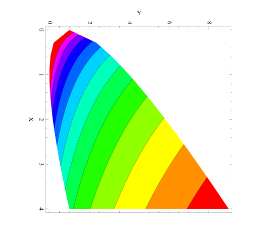
The form of the shape function in (50)-(57) determined from conformal invariance of flat sections in de Sitter space is quite different from that derived from the simplest inflation models [10, 32, 33]. For example, the parameterization of the non-Gaussian term in single field slow roll inflation by a small non-linear term, , where is the non-linearity parameter, leads to the “local” model of the dimensionless non-Gaussian shape function,
| (58) |
where is the normalization of the two-point power spectrum for the inflaton or gravitational potential fluctuations during slow roll. The “equilateral” shape,
| (59) |
has also been considered by some authors, while the full prediction for the bispectral shape for single field slow roll inflation is the linear combination [33]
| (60) |
with
| (61) |
the usual slow roll parameters defined in terms of the scalar inflaton potential and its derivatives.
Clearly these shape functions are quite different from (50) for general or , or (57) for , degenerating to each other only in special kinematic configurations. The reason for this is that the standard assumptions of slow roll inflation models require a departure from de Sitter space and violation of conformal invariance. Only (approximate) scale invariance is assumed, which as we have observed gives (45) which does not completely fix the form of the bispectrum. In addition, in the usual picture the magnitude of non-Gaussianity of the CMB is tied to the violation of de Sitter and conformal invariance parameterized by the slow roll parameters, whereas (50) or (57) is derived from the intrinsic conformal symmetries of de Sitter space itself, with an amplitude that is otherwise undetermined by conformal invariance considerations alone. It is therefore possible for both the magnitude and the shape of primordial non-Gaussianities in the CMB to be quite different from models tied to the slow roll of scalar inflaton field, and for observational detection of an alternate form of the shape function to point to a quite different dynamical origin for the CMB fluctuations. We note also that (58), (59) or (60) are quite singular as one of the , whereas (50) has at worst a logarithmic behavior in this limit. This implies that observational limits on the amplitude of the slow roll shape (60) will generally lead to less restrictive limits on the amplitude of the non-Gaussian bispectrum (50).
For higher point correlations, the conformal invariance identities (41) do not completely determine the correlation functions [11]. For , the solution of (41) is
| (62) |
where is an arbitrary function of the two cross-ratios, and . Analogous expressions hold for higher -point functions. In the equilateral case in Fourier space, , the coefficient amplitudes become constants and one again obtains a universal dependence in the limit .
IV Gravitational Potentials and Their Scaling in de Sitter Space
In this section we derive the relationship between energy density perturbations and scalar gravitational potential perturbations in de Sitter space, in a fully relativistic gauge invariant formalism. In so doing we justify (32), showing how the density perturbations of conformal weight in the deS/CFT approach generate the scale invariant HZ spectrum for the gravitational potentials, and hence the CMB temperature anisotropies at large angular scales, where the Sachs-Wolfe effect dominates
The fluctuations around any self-consistent solution of the semiclassical Einstein eqs. satisfy the linear response eqs.,
| (63) |
These couple the fluctuations of the metric to the fluctuations of the quantum matter stress tensor, at linear order in the deviation from the de Sitter metric , i.e.
| (64) |
It is well known that the metric perturbations which are scalar with respect to the background three-metric in the flat FLRW coordinates (1) can be parameterized in terms of functions, , in the form [34, 35, 8],
| (65a) | |||||
| (65b) | |||||
| (65c) | |||||
Since the linearized metric perturbation under a linearized coordinate (gauge) transformation undergoes the change
| (66) |
and in the space plus time split the gauge transformation can be characterized by scalar functions and , it follows that only linear combinations of the functions in (65) are gauge invariant. These may be taken to be the gauge invariant gravitational potentials
| (67a) | |||
| (67b) | |||
These are the gauge invariant gravitational potentials denoted by and in ref. [34], and by and in Ref. [35], while the authors of ref. [8] employed the notation for .
The general stress-energy tensor perturbation in flat FRLW coordinates in the scalar sector may be decomposed according to the analog of (65) for the metric tensor. Thus we specify the stress tensor components in the scalar sector in terms of functions by
| (68a) | |||
| (68b) | |||
| (68c) | |||
We note that the stress tensor perturbations around exact de Sitter space are gauge invariant [8], and hence so are the functions . However, invariance under the coordinate gauge transformation (66) implies that the scalar functions are not all independent, but rather are related by non-trivial constraints embodied in the conservation eqs.
| (69a) | |||
| (69b) | |||
corresponding to the coordinate gauge symmetries specified by . There remain independent stress tensor components in the scalar sector and the information needed to determine the gauge invariant potentials in terms of these is contained completely in the and total trace components of the linearized Einstein eqs.,
| (70a) | |||
| (70b) | |||
the other components of the linearized Einstein eqs. being automatically satisfied if the Einstein eqs. for the background and stress tensor conservation eqs. (69) are satisfied [36].
Specializing to de Sitter space where is a constant and the energy density and pressure perturbations are themselves gauge invariant for arbitrary spatial dependence [8], the two relevant linearized Einstein eqs. (70) may be written in the gauge invariant form [36]
| (71a) | |||
| (71b) | |||
By differentiating (71a) with respect to and operating on it with , and then taking appropriate linear combinations with (71b), these eqs. may be solved for the gravitational potentials in terms of and in the form
| (72a) | |||
| (72b) | |||
When the conservation eqs. (69) are used, we see that the right sides of (72) are proportional to total spatial Laplacians, one of which therefore may be cancelled from each side of eqs. (72), with the simple result
| (73a) | |||||
| (73b) | |||||
in the sector with non-vanishing spatial derivatives, or in Fourier space . The sum and difference of eqs. (73) give
| (74a) | |||
| (74b) | |||
showing that if there are no anisotropic spatial stresses, , the gravitational potentials are equal and opposite in the spatially inhomogeneous sector, or in the notation of [8].
In the spatially homogeneous sector , we may set , there is only one gauge invariant potential, namely which is given directly by (71a), and (71b) is automatically satisfied because of the remaining conservation eq. (69b) with . This degeneracy of the case is related to the existence of () conformal Killing vectors in de Sitter space, which being composed of linear combinations of constant, linear () and quadratic () functions of the spatial coordinate, are non-Fourier normalizable at , where the Laplacian is non-invertible. The existence of these conformal Killing modes implies that there is an enhanced linear diffeomorphism symmetry and hence fewer gauge invariant potentials at . This connection can be shown most clearly by working in the spatially closed coordinates of (160), for which the spatial Laplacian has a discrete spectrum, all the modes are normalizable on , and the degeneracy in the gravitational potentials and conformal Killing vectors appear together in the (singlet) and (quartet) harmonics on [37].
The result (73) shows that the relativistic gravitational potentials in linear perturbation theory around de Sitter space are related to the stress tensor sources in the scalar sector in the same manner as in Newtonian theory, namely by the Laplacian of the non-relativistic Poisson eq. The only differences from the non-relativistic case are the appearance of two potentials in the relativistic theory rather than one when anisotropic stresses are present (i.e. ), and the appearance of the velocity perturbation as an additional source of the relativistic potentials. Note that no assumption about the perturbations being sub- or super-horizon has been made. Eqs. (73) are exact gauge invariant relations in the flat FRLW coordinates (1) of de Sitter space.
From the discussion in Sec. II, a density perturbation of weight redshifts at large cosmological time in the asymptotic conformal scaling region of de Sitter space according to
| (75) |
If the other components of the general stress tensor perturbation (68) scale the same way at late cosmological time , then from the solution (73) under dilations the gravitational potentials scale according to
| (76) |
in the asymptotic region of de Sitter space. This establishes the scaling weight of the potentials in terms of the energy density perturbations in the scaling region. In particular it shows that the scaling weight of the gravitational potentials necessary to give rise to a scale invariant Harrison-Zel’dovich spectrum of CMB temperature anisotropies must arise from a conformal weight energy density perturbation in de Sitter space. Such behavior has been found in the energy density perturbations of a massless, minimally coupled scalar field in de Sitter space [38], exactly as expected on general grounds from (27) and (28) for and . Let us emphasize again that these are quantum fluctuations intrinsic to de Sitter space, with vanishing expectation value of the scalar field , and no slow rolling inflaton.
We have used the notation for the gravitational potential scaling dimension (76) because it is not a conformal weight in the same sense as . The reason is that the Laplacian is not a conformal differential operator in dimensions (as it is in dimensions). Thus the gravitational potentials from the linearized Einstein eqs. satisfying (73) are not conformal fields possessing well-defined transformation properties under the special conformal transformations (44). This has no effect on the two-point power spectrum (33), whose form is determined by global dilations alone, without the full conformal group. The power of needed to convert energy density fluctuations to gravitational potential fluctuations (hence CMB temperature fluctuations), which follows from (73) and global scaling under dilations is all that is needed to convert the power spectrum of density perturbations to that of the gravitational potential in de Sitter space.
The non-convariant transformation properties of in dimensions does mean that treating the energy density as a conformal field with conformal weight , whose three-point correlator is given by (47) or (48)-(51) in Fourier space, satisfying the Ward identity (46), and then dividing by according to (78), is not equivalent to treating the gravitational potentials and CMB temperature fluctuations themselves as conformal fields of weight . This is obvious from the fact that treating the energy density as a conformal field with a definite weight gives
| (77) |
leading to eq. (52) of the previous section for the CMB bispectrum, while the second prescription of treating the gravitational potential(s) and CMB temperature fluctuations themselves as conformal fields of weight would give
| (78) |
Clearly (77) and (78) and their corresponding shape functions are quite different including in the squeezed limit, although they have the same overall scaling under global dilations of all vectors simultaneously if is given by (76). This is the reason that the authors of [39] obtained a different result for the squeezed limit of the non-Gaussian CMB bispectrum under the second hypothesis than we have obtained under the first hypothesis of treating as a conformal field of weight near , rather than any error in evaluating the integral in terms of hypergeometric functions, either in Sec. III or [39].
V The Static Frame and Conformal Invariance on the de Sitter Horizon
The embedding of the flat spatial coordinates (1) is one way in which conformal invariance can be realized in de Sitter spacetime. The use of flat spatial sections is not essential in fact. The conformal group of the closed and open hyperbolic spatial sections in cosmological coordinates is also the de Sitter isometry group . Hence the main results apply to all cosmological homogeneous and isotropic metrics whether the spatial sections are open, closed or flat.
In this section we consider a rather different realization of conformal invariance from embedding in de Sitter space based on the existence and kinematics of the cosmological horizon. The leads to a different set of conformal Ward identities and a different form for the CMB non-Gaussian bispectrum, as well as a rather different suggestion for the physical origin of CMB anisotropies, and models of dark energy. As in the previous case, the basic kinematics is best illustrated by exhibiting explicit coordinates. In this case we make use of the static coordinates of de Sitter space (reviewed in Appendix A) .
In the static coordinates the line element of de Sitter spacetime can be expressed in the form
| (79) |
These static coordinates are quite different from the spatially flat FLRW coordinates (1) globally. Rather than exponentially expanding, the metric in (79) is independent of time . Rather than being spatially homogeneous, the static coordinates have a preferred origin about which they are rotationally invariant. The horizon for the observer at is apparent in (79) as the spherical surface at where the line element becomes singular. Notwithstanding their rather different forms, the line element (79) is a representation of de Sitter spacetime equally valid to the FLRW line element (1) in their region of common applicability within the observer’s cosmological horizon.
The explicit coordinate transformations from flat FLRW coordinates (1) to static coordinates (79) are given by Eqs. (227)-(228) of Appendix G. Note in particular from (227)
| (80) |
so that the distant past corresponds to either or . Hence in a de Sitter universe (or a universe dominated by dark energy which approximates a de Sitter universe) primordial fluctuations usually thought of as arising in a very early epoch in the history of the universe, may in fact arise on or near the cosmological horizon at instead.
Note next that in the static frame the metric factor
| (81) |
so that the static time variable drops out completely at the horizon. The invariant distance function in de Sitter space defined previously by (11) becomes in the static coordinates (79)
| (82) |
where are the two unit direction vectors on the sphere. Eq. (82) shows that if the two points are on the horizon with respect to the origin of static coordinates, then this function becomes simply
| (83) |
and the de Sitter invariant function when both points are on the horizon is a function only of the invariant quantity on the sphere, namely .
That the cosmological horizon is also the locus of conformal behavior may be seen in several different ways. On the static const. hypersurfaces the remaining three dimensional line element of (79) takes the form
| (84) |
where and
| (85) |
Hence the horizon at is mapped to in these coordinates, and the line element within the square brackets of (84) may be recognized as a standard form of three dimensional Łobachewsky (Ł) or Euclidean Anti-deSitter (EAdS3) space, consisting of one sheet of the doubled sheeted hyberboloid with isometry group . Thus, by well-known arguments of AdS/CFT correspondence [40], one expects conformal behavior at the two dimensional horizon boundary, namely on the sphere of directions with [17]. This conformal behavior can be seen most clearly by introducing Poincaré coordinates for the three dimensional optical metric, viz.
| (86a) | |||
| (86b) | |||
| (86c) | |||
so that the three dimensional Łobachewsky metric in (84) takes the standard Poincaré form
| (87) |
In these Poincaré coordinates the two dimensional horizon boundary manifold at has been mapped into the plane, parameterized by , by stereographic projection [17]. The north pole at and is mapped to the point at . It is clear from (87) that scale transformations of the plane at fixed can be compensated by a corresponding simple scale transformation on . This is an exact symmetry of the three dimensional Łobachewsky metric. When this scale transformation is supplemented by the two special conformal transformations of , one obtains the full global conformal group of either or , namely , which is exactly the isometry group of the three dimensional Łobachewsky space .
On the action of can also be represented as the group of proper Lorentz transformations acting on the directions of radial light rays in dimensions, c.f. Appendix E. In de Sitter space this is the subgroup of the de Sitter group that leaves the static time and three dimensional metric (84) invariant. Again the conformal group of a dimension slicing is isomorphic to the symmetry group of the embedding dimensional space, with now . Since , the mapping of Killing vectors of de Sitter spacetime to conformal Killing vectors on cannot be one to one, but there is a projective (several to one) mapping, which is described in detail in Appendix C. Hence conformal transformations of the spherical horizon boundary metric at can be viewed as coordinate transformations which leave the three dimensional de Sitter metric at constant invariant, and conformal invariance on the cosmological horizon follows from de Sitter invariance of the bulk, just as in the embedding considered previously.
The conformal behavior at the cosmological horizon of de Sitter space in the static frame may viewed in another way. In coordinates (79) because of the dependent compression of physical time , there is the usual kinematic gravitational redshift/blueshift of the local frequency
| (88) |
measured at relative to that at the origin. The corresponding energy diverges as and therefore becomes much greater than any finite mass scale, which may be neglected at the horizon. As shown in Appendix E this is reflected in the fact that the wave equation for a scalar field of arbitrary finite mass (25) becomes indistinguishable from that of a massless conformal field in the horizon limit . Thus conformal behavior in this limit is to be expected on physical grounds of all mass scales becoming negligible.
The three dimensional line element (87) has a form quite analogous to the four dimensional de Sitter line element (13) with the spacelike coordinate taking the place of the conformal time , and with the boundary in (87) at taking the place of the boundary in (13) and Figs. 5-6 at , . Thus the analysis of conformal behavior at the horizon boundary parallels the corresponding late time behavior of the FLRW flat embedding. The scale transformation is analogous to (10) in the full de Sitter metric (13) in its Poincaré conformal time coordinates. As in (26) this makes possible the study of conformal behavior of fields or correlation functions on the horizon boundary by the scaling behavior with in the corresponding bulk Poincaré coordinate. Although the representations of the conformal group generated at fixed need not be simple or irreducible in general, as the horizon boundary is approached, , , simple power law behaviors and definite conformal weights can be produced. This conformal weight of a field can be obtained by examining its power law behavior [40]
| (89) |
near the horizon boundary. Further, since the invariant distance function on Łobachewsky space, analogous to (14) is
| (90) | |||||
which is conformally related to the de Sitter invariant distance function (82) with , we see that positive conformal weight fields with with scaling behavior (89) will have two-point correlation functions on the horizon sphere with the angular behavior
| (91) |
with
| (92) |
analogously to (22). This is a key result which we shall make use of in the next section.
VI CMB Power Spectrum and Bispectrum on the de Sitter Horizon
Since the physical origin of fluctuations generated after many -foldings in an inflationary epoch on the one hand, and those generated on or near the cosmological horizon on the other are quite different, they lead to quite different observational consequences for CMB non-Gaussianity. To derive the form of the conformal Ward identities in this second case we make use of the representation of the conformal group of the sphere as the proper Lorentz group in three spatial dimensions described in Appendix E In fact, the conformal transformations of the directions on the sphere regarded as light rays may be placed in one-to-one correspondence with Lorentz boosts [14]. The infinitesimal form of this conformal transformation parametrized by the Lorentz boost velocity vector in (207) or (210) is
| (93) |
For the two-point correlation function of a conformal field with weight , rotational invariance first restricts to be a function only of the invariant (83). Then the conformal identity is
| (94) |
or using (209) in infinitesimal form, we have
| (95) |
where denotes the gradient with respect to on the sphere and similarly denotes the gradient with respect to . From (83) on the de Sitter horizon
| (96) |
so that
| (97) |
and similarly for . Hence
| (98) |
Thus implies that satisfies
| (99) |
which has the solution
| (100) |
It is also straightforward to show from the finite transformation (210) that on the horizon
| (101) |
with given by (209). When raised to the power this verifies (94) directly.
Turning next to the three-point function of three fields of equal conformal weight,
| (102) |
invariance under the conformal transformation (207) implies
| (103) |
or in infinitesimal form,
| (104) | |||||
This condition can be satisfied for arbitrary if and only if
| (105) |
Therefore, the conformal Ward identity (104) requires
| (106) |
for some constant . This procedure may clearly be continued to higher point functions, with the results similar to flat space with replaced by . Again the form of the four point trispectrum is constrained but not uniquely determined by conformal invariance.
Unlike the case considered previously where the conformal invariance of -point functions was assumed to pertain on the flat sections of a FLRW cosmological model, and has to be translated first to Fourier space and then finally to angular directions on the sky of the CMB, (106) gives the form of the non-Gaussian bispectrum directly in angular variables, as observed from the origin of the static de Sitter coordinates (79). This corresponds to treating the present universe as approximately de Sitter due to the dominance of dark energy today, and the CMB anisotropies as generated by de Sitter invariant fluctuations on the cosmological horizon, rather than having re-entered the Hubble sphere from an earlier inflationary phase. We discuss in the next section a possible physical mechanism which could provide these conformal fluctuations on the cosmological horizon of de Sitter space.
If one parallels the discussion in the FRLW case considered previously, one would again start with energy density fluctuations of conformal weight , and then convert these to fluctuations in the gravitational potentials in the scalar sector by solving the linearized Einstein eqs. according to (71)-(74). An important difference from the previous case is that whereas the Laplacian is not a conformal differential operator on , it is conformal when restricted to . Thus the solution of the linear response eqs. (71)-(74) will yield conformal scalar potentials that transform under the conformal group of , with definite conformal weights, , rather than only under global dilations only. We will give an explicit example of this in the next section.
In addition, in a cosmological model of this kind, the observable CMB power spectrum may be obtained directly in terms of the angular variables on the sky from conformal field(s) of definite conformal weight (or nearly zero), without any need of the passing through the intermediate step of spatial Fourier transforms on . Inspection of (91) or (100) shows that that a weight field on has an angular correlation function
| (107) |
which is exactly the angular correlation of the classical Harrison-Zel’dovich CMB spectrum (37) in the Sachs-Wolfe regime. Thus, at the level of the two-point power spectrum alone one cannot distinguish this radically different possibility for the origin of the CMB anisotropies and power spectrum from the standard FLRW cosmological model. In other words the observable CMB two-point power spectrum is identical in the three quite different physial models:
- 1.
The usual slow roll inflation scenario of CMB temperature anisotropies exiting and then reentering the cosmological horizon;
- 2.
- 3.
A scale invariant Gaussian CMB power spectrum with conformal weight nearly zero, and logarithmic correlations on as in (107) is obtained from slow roll inflation, or from the conformal invariance inherited from de Sitter invariance, whether we regard the primordial fluctuations as arising on or embeddings in a dark energy dominated universe, such as that postulated in inflation, or even as applies to the observable universe today for a much lower value of . The details of the CMB power spectrum such as the acoustic peaks will be produced in the interior of the cosmological horizon by the same causal physics in any case, no matter how the primordial fluctuations were generated, whether on or from beyond the Hubble sphere. Thus the two-point power spectrum alone cannot provide definitive evidence of detailed inflationary scenarios or the origin of the CMB anisotropies.
When one shifts attention to the non-Gaussian correlations, the situation is quite different. The bispectrum in the case (106) becomes in limit
| (108) |
which is completely separable, and quite different again from either (57) or the single field slow roll inflation prediction (60). In fact, in this limit (108) is ultralocal, in the sense that the shape function corresponding to it in the flat Fourier space variables of the previous section has an additional function. To see this, note that in flat coordinates
| (109) |
if the two points from which the CMB photons are emitted are (neglecting fluctuations) at the same physical distance, as usually assumed in the standard cosmological model. Inserting (109) into (108) for each of the factors, and Fourier transforming with respect to each of the position variables gives
| (110) |
where again . Extracting an overall and multiplying by to compare with the dimensionless shape function of a conformal weight field in (50) we find that the result is proportional to
| (111) |
which has support only when one of the , i.e. in the squeezed configuration. If one takes slightly greater than in (106), this extreme concentration on the squeezed configuration is smoothed somewhat, but should still be distinguishable from the local shape function (58). If non-Gaussianities are detected in the CMB, and in particular the support of the bispectral shape function is found to be highly peaked on the squeezed configuration, consistent with (108) or (111) for low multipoles, it would be evidence in favor of conformal invariant origin of the CMB anisotropies on the cosmological horizon, as described in this section. If the shape of the primordial bispectrum can be determined (irrespective of magnitude), the three different possibilities for the spacetime locus and origins of the fluctuations themselves may be distinguished by observations. The bispectrum a generic freely falling observer at a point offset from the origin would see may be worked out with simple geometric considerations and will be presented elsewhere.
VII CMB Anisotropies from Cosmological Horizon Modes
Up until this point we have simply assumed the existence of scalar fluctuations in de Sitter space, which couple to the gravitational field, and worked out the purely kinematic consequences of that assumption. As is well known there are no scalar fluctuations in the classical Einstein theory. Thus if we are to do away with the scalar inflaton, the question naturally arises of what supplies the necessary scalar degree of freedom in its place. In this section we discuss a possible quantum origin and physical mechanism for the generation of scalar fluctuations in de Sitter space, which could give rise to the CMB anisotropy and non-Gaussianities on the cosmological horizon, as discussed in the last section. For this we first recall some properties of quantum fields and their fluctuations in de Sitter space.
The first observation is that the de Sitter invariant state with correlation function (17) is in fact a thermal state with respect to the static time coordinate of (79). Mathematically this follows from the fact that de Sitter invariant correlator is periodic in imaginary time , as is immediately obvious from (83) and the periodicity property of the hyperbolic function, cosh. The resulting periodicity of the correlator (17) is exactly the KMS condition for a propagator in thermal field theory [41], with the temperature [42]
| (112) |
In the de Sitter invariant equilibrium state the radiation entering the horizon volume is exactly compensated by the radiation leaving it, so there is no net flux and the state is stationary with respect to the Killing static time .
When one considers next fluctuations around the equilibrium state, it is natural to consider causal fluctuations in the temperature within one horizon volume. At that point one immediately finds a perhaps surprising result: any finite temperature fluctuation in the spherical volume enclosed by away from the equilibrium value (no matter how small) produces an infinite stress-energy tensor at the horizon. Indeed the expectation value of the renormalized stress-energy tensor has the form [43]
| (113) |
as . The quadratic power divergence in this limit can be understood from the kinematic blueshift (88) and the fact that the stress tensor is a dimension operator, and so scales as . The divergence in (113) vanishes if and only if i.e. if and only if all fluctuations in the temperature within any given horizon volume are identically zero. Note that if such a fluctuation does occur it would spontaneously break the larger de Sitter isometry group to a subgroup or , selecting from the homogeneous ensemble where any point is equivalent to any other, a preferred origin at around which the fluctuation is centered [44].
The quantum matter source on the right side of (63) that gives rise to these fluctuations can be described by an effective action functional, the relevant part of which can be written in the form,
| (114) |
in terms of a new scalar field . Here
| (115a) | |||||
| (115b) | |||||
| (115c) | |||||
in terms of the number of the underlying massless quantum conformal scalar (), Weyl fermion () and vector () fields contributing to the quantum stress tensor. The fourth order differential operator is conformally invariant (when multiplied by ) and factorizes in de Sitter spacetime as indicated in the last form of (115c). Let us emphasize that the scalar due to the trace anomaly is not introduced as adding new inflaton degrees of freedom in a model dependent way, but rather is the result of quantum fluctuations of Standard Model massless fields (such as the photon, or the graviton itself) in curved space with no additional assumptions. The field is a purely quantum scalar degree of freedom over and above the classical transverse, traceless degrees of freedom in General Relativity. It can be understood as describing two-body correlations of the underlying quantum theory [45].
In ref. [36] the solutions of eqs. (63) with the stress-energy tensor derived from (114) were studied in both the flat FLRW coordinates (1) and the static coordinates (79). Linearized perturbations of the stress tensor of the form (113) were found, corresponding to the fluctuation of the thermal state away from its strict Hawking-de Sitter value (112). The large effects on the stress tensor at the de Sitter horizon as in (113) are due to the perturbations of the anomaly scalar in the one-loop effective action (114). Note that the stress tensor of these fluctuations need not become infinite on the horizon, but only sufficiently large to influence the de Sitter geometry through the semiclassical Einstein eqs. (63), which couple the metric perturbation to the fluctuations of the anomaly scalar .
In order to determine how the perturbations of stress tensor due to the trace anomaly behave under conformal transformations in de Sitter space, and find their conformal weights, we apply the general method of Sec. IV to the these fluctuations of , first in the flat FRLW coordinates (1) and then on the de Sitter horizon sphere. In the coordinates (1) the linear response equations in de Sitter space are of the form (71) with
| (116) |
where the quantity is the effect of the quantum matter source, given in terms of the gauge invariant perturbation of the anomaly scalar field in (114) by the relations [36]
| (117a) | |||||
| (117b) | |||||
The condition (116) with (71b) implies that the linearized perturbation in the Ricci scalar vanishes, , which removes the possibility of very high frequency Planck scale perturbations from the fourth order operator , and guarantees that the remaining solutions of (71)-(117) are in the long wavelength regime of validity of the semiclassical eqs. far below the Planck scale in energy. Thus (71) with (117b) are finally second order equations for with no Planck scale solutions. The solutions of (117b) in flat FLRW coordinates are
| (118) |
in which the gravitational constant enters only through the combination describing the weak coupling of the quantum anomaly to the metric perturbation in (71) for a macroscopically large de Sitter space.
Note that these modes (118) solving the anomaly scalar eqs. (117) describe an additional effective scalar degree of freedom, arising from the purely quantum effects of the trace anomaly, which act as linearized sources to the usual gravitational potentials in the scalar sector of linearized gravity, without introducing an inflaton field. Thus whereas in the purely classical theory with , there are no dynamical scalar degrees of freedom and the only solutions of (71) with are trivial, once the anomaly scalar degree of freedom drives fluctuations in the gravitational potentials much as scalar inflaton fluctuations do in the conventional picture. In contrast to the conventional picture these are generated by quantum fluctuations described by the anomaly effective action (114), and are intrinsic to de Sitter space, requiring no fine tuned inflaton potential or slowly rolling classical expectation value of a de Sitter breaking inflaton field.
Using the conservation eqs. (69) and (117b) we find for the other components of the anomaly stress tensor in the scalar sector defined in
| (119a) | |||
| (119b) | |||
Thus using (73) the solution of the linear response eqs. for this anomaly scalar perturbation is
| (120a) | |||
| (120b) | |||
for the sum and difference of the gravitational potentials for spatially inhomogeneous perturbations, in Fourier space . Since for , the first of these relations show that the sum of the gravitational potentials has a scaling dimension in the conformal scaling region of de Sitter space at late FRLW time. Thus this combination cannot give rise to the scaling needed (namely, ) for an approximately flat Harrison-Zeld’ovich spectrum of CMB fluctuations. For the second linear combination of potentials, in (120b), inspection of (118) shows that the differential operator on the right side of (120b) reduces its behavior to for , so that the difference of potentials has the scaling dimension at late FRLW time, again not the behavior needed for generating a flat CMB spectrum. Thus we conclude that the scalar degree of freedom present in the quantum trace anomaly does not generate the observed spectrum in the first realization of conformal invariance in de Sitter space in the flat FRLW sections (1) at late times.
This negative result is a consequence of the special role that the strictly homogeneous mode with plays in the FRLW case, and the existence of the conformal Killing vectors of de Sitter space, which lead to enhanced gauge symmetry at and to non-invertibility of the scalar Laplacian in (120b) in the scaling region, . The additional coordinate gauge modes at the singular limit in flat FRLW coordinates also preclude any use of the homogeneous modes of the gravitational potentials to extract their scaling dimensions along the lines of (26). In the second realization of conformal invariance on the de Sitter horizon, as shown explicitly in Appendix C, the Killing vectors of de Sitter space (185)-(189) do not have non-trivial harmonics on , so that the Laplacian on is invertible, and the linearized Einstein eq. (120b) for the difference scalar gravitational potentials is solvable (up to a harmless constant). The conformal weight may be also obtained for this linear combination of gravitational potentials by a method analogous to (26) in the static coordinates, as we shall now show.
In the de Sitter cosmological horizon limit , we can find the conformal weights of and scaling of by converting the differential operators in (117b) and (120b) to static coordinates (79), and examining the functions of only obtained in the horizon limit. Since is related to of the Poincaré coordinates (86) by (86c), and conformal weights obtained from (89) are necessarily tied to the behavior of correlation functions on by (91) through de Sitter invariance, this is the precise analog of obtaining conformal weights through the simple time dependence of spatially homogeneous functions via (26) in the FRLW case.
Using the explicit forms of the coordinate transformations in Appendix G and assuming that are now functions only of the static radius , (117b) becomes
| (121) |
which has the general solution [45, 36]
| (122) |
for some constants and . Now the scalar Laplacian in (72) is invertible without any problem (up to constant and solutions, the first of which is harmless and the latter of which is singular at and hence excluded). Thus eqs. (120) hold and (120b) becomes
| (123) |
which has the general solution
| (124) |
again up to solutions of the homogeneous eq. . In static coordinates these solutions are , so that they are either singular at , or give an irrelevant finite additive constant at .
Now the result (124) shows that the difference of gauge invariant gravitational potentials behaves logarithmically on the de Sitter horizon. Since in the case that all the potentials are functions only of the static radial coordinate , and by (89) conformal weight fields scale like as , the logarithmic scaling with in (124) corresponds to conformal weight
| (125) |
In the case the scaling dimension is also the conformal weight under the conformal group on the horizon.
Hence the conformal anomaly scalar in (114), itself a fluctuating scalar degree of freedom drives the difference of gravitational potentials (124) at linear order in perturbations around de Sitter space, and provides a possible source for zero conformal weight fluctuations that can give rise to the correct scale invariant Harrison-Zel’dovich angular correlations at low multipoles according to (37) and (107). The result (120a) for the sum of gravitational potentials shows that this linear combination gives scaling dimension according to (89). A negative conformal weight means that this combination cannot give rise to well-defined unitary conformal field on the de Sitter horizon. It suggests instead unstable or tachyonic behavior that requires a study of of the fully time dependent solutions of (72). We note that projecting onto the logarithmic weight zero terms requires equal and opposite gravitational potentials , which interestingly is just the same linear combination generated by hydrodynamic perturbations (with no anisotropic stresses) in slow roll inflation models [8]. It is the combination of zero scaling dimension under global dilations that can give rise to the HZ spectrum.
The logarithmic power correlation function on the sky (107) derives from that of the anomaly scalar field of zero conformal weight in (114). Indeed the propagator for is the inverse of the operator defined by (115c). Since in de Sitter space factorizes, this propagator can be written as
| (126) |
where
| (127) |
is the propagator of a massless, minimally coupled scalar field (on the space of non-constant modes) and is the propagator of the massless, conformally coupled field (16). Thus from (199), (126), and (127),
| (128) |
is a pure logarithm, up to an arbitrary additive constant. From (83) on the de Sitter horizon,
| (129) |
where is the cosine of the angle between the two direction vectors on the sky viewed from the origin from which the radiation appears to originate. This correlator is that of the two dimensional conformal Laplacian operator on the sphere . This is the conformal weight zero logarithmic correlator that is transmitted to the difference of gravitational potentials by the semiclassical Einstein eq. (63) and therefore to the CMB temperature fluctuation power spectrum through the Sachs-Wolfe effect for large angular scales, i.e. low multipole moments. Thus the anomaly scalar fluctuations governed by (117) can give rise to the CMB power spectrum in a fully conformally invariant way on the de Sitter horizon, without any need of the ad hoc introduction of a scalar inflaton field.
Since the form of the two-point correlation function is dependent upon the conformal weight of the field giving rise to the fluctuations, and not upon the detailed dynamics, observations of the two-point correlations of the CMB anisotropies alone cannot distinguish (107) arising from fluctuations on entering the horizon with spectral index from those of (128), arising from fluctuations of the anomaly scalar field and near the cosmological horizon itself. These globally radically different physical origins lead to the same gauge invariant gravitational potentials, and generate the same Harrison-Zel’dovich large angle CMB power spectrum directly on the sky, (37), (107) or (129), for an observer at or near the origin . As shown in Secs. III and VI the CMB bispectrum can be used to distinguish these different possible origins. The corrections to this angular form from displacements from the origin vanish at first order and will be presented in a separate publication.
VIII Gravitational Waves from Conformal Invariance
The considerations of conformal invariance can be extended equally well to the spectrum of gravitational waves. The fundamental quantity is the correlation function of transverse traceless tensors,
| (130) |
where given by
| (131a) | |||||
| (131b) | |||||
is the projector onto transverse traceless tensors in flat Euclidean . Eq. (130) is the general form of the spin-2 gravitational wave correlation power allowed by conformal invariance with a general spectral index and overall amplitude , which may be obtained by solving the conformal Ward identity relations analogous to (41) leading to (23). Since the projector is invariant under scaling , simple power counting in shows that the spin-2 correlator in position space (130) must take the form
| (132) |
for some other constant . One can find the full spin-2 conformal correlation function in position space, obviating the need to construct the projector separately, by following a method for maximally symmetric spaces parallel to that for the de Sitter space graviton two-point function [46].
To this end note first that translational and rotational invariance in requires the full spin-2 correlator to be a function only of the unit vector
| (133) |
and the invariant distance
| (134) |
Then noting that there are exactly four-index tensors symmetric under interchanges of and , and , and the interchange of the pair and , that can be constructed out of the unit vector and the flat space metric , namely
| (135a) | |||
| (135b) | |||
| (135c) | |||
| (135d) | |||
| (135e) | |||
one can expand in this basis set of tensors multiplied by arbitrary scalar functions of ,
| (136) |
The minus sign in (135e) is in order to agree with the conventions of [46]. Then using
| (137) |
and imposing the conditions of tracelessness and transversality,
| (138) |
one can derive independent conditions on the functions , viz.
| (139a) | |||
| (139b) | |||
| (139c) | |||
| (139d) | |||
where a prime denotes the derivative with respect to and we have defined the linear combinations
| (140a) | |||
| (140b) | |||
Now if we assume the power law dependence,
| (141) |
which defines the tensor scaling exponent in terms of the spectral index,
| (142) |
then (139) and (140) may be solved for all scalar functions with the same power law in the form,
| (143) |
with
| (144a) | |||
| (144b) | |||
| (144c) | |||
| (144d) | |||
| (144e) | |||
The constant is then fixed in terms of by identifying the coefficient that multiplies the tensor (which does not involve ) with the same tensor structure in (130). Recalling (131b) this gives
| (145) |
where is defined by
| (146) |
so that
| (147) |
For we have
| (148) |
as . As in the scalar case, (37) the zero weight limit produces a pole term in position space if the momentum space normalization is held fixed, and this pole term must be subtracted to obtain the normalization in the logarithmic case. The tensor correlation (130) or (132) may likewise be converted into a correlation of gravitational waves on the directions of the sky by assuming as in (33) that the emission points are at equal distance from the observer.
As in the case of scalar perturbations, the same result for the two-point correlation (130) or (132) is obtained whether one employs the conformal Ward identities inherited from de Sitter invariance to the spatial slices of FRLW cosmology at fixed cosmological time , or those of the subgroup of conformal transformations on the de Sitter horizon sphere at fixed de Sitter static time . Either way, once produced, the gravitational waves will propagate within our cosmological horizon and affect the CMB photon polarization and particularly the -modes by the same scattering processes as those extensively investigated in present models [27, 47].
Now if one and the same physical mechanism is responsible for the conformal invariance of both the scalar and tensor perturbations, as each are components of the same four dimensional spacetime linearized metric perturbation , one would expect them to have the same conformal scaling dimensions,
| (149) |
Taking into account the definitions of the scalar and tensor spectral indices, (30)-(32) and (142) respectively this implies
| (150) |
The validity of this relation depends upon the effective theory of the origin of the scalar and tensor fluctuations having non-vanishing lowest conformal weight representations. Thus, we have argued that the lowest conformal weight scalar density perturbations should be , and these lead generically to the scalar gravitational potentials having scaling dimension according to the linearized Einstein eqs. (32). This scaling dimension is actually realized for the scalar gravitational potentials in the realization of conformal symmetry in de Sitter space (125).
Correspondingly, the metric tensor perturbations in the transverse, traceless sector are well-known to behave like a massless, minimally coupled scalar field in de Sitter space, and so according to (19) and (26), the tensor modes have as well. Indeed their propagator in de Sitter space behave logarithmically with large invariant distance [46], just as would be expected for a field. It would be interesting to check this logarithmic scaling of the tensor two-point function on the cosmological horizon realization of conformal symmetry in de Sitter space. This relation of scalar and tensor spectral indices could furnish an important check on the proposed origin of the CMB from conformal invariance as we have been considering in this paper, and in particular of the realization of conformal invariance on the cosmological horizon of de Sitter space from the quantum fluctuations of the anomaly.
Note that the the equality of spectral weights and the relation (150) between the spectral indices of the scalar and tensor fluctuations expected from considerations of conformal invariance in de Sitter space differs from the predictions of slow roll inflation models where the scalar and tensor spectral indices have different dependences on the slow roll parameters [7]. In practice the deviations of each spectral index ( in the scalar case and in the tensor case) is predicted to be very small, so this may be a difficult difference to detect. Conversely, if the spectral indices of the scalar and tensor perturbations are found to differ measurably from the conformal expectation (150), this would certainly make less plausible a common origin of the scalar and tensor fluctuations by conformal invariance. For a treatment of tensor modes in the slow roll model see [48].
As in the scalar case, conformal invariance alone does not predict the amplitude of the gravitational wave component, provided they are small in magnitude so that a well-defined geometrical background such as de Sitter space with its classical symmetry group applies. For that one needs a concrete dynamical realization of conformal symmetry, such as the one proposed in Sec. VII [49]. In the semi-classical limit where fluctuations around the background are small, one would also expect the anomalous deviations from naive classical conformal scaling dimensions to be be small, and hence .
Present observations indicate that that (from WMAP data alone, with the uncertainty estimate reduced to if all relevant cosmological data is fit [4]). Thus a value slightly less that unity is currently preferred, whereas the conformal invariance hypothesis would seem to favor positive anomalous dimensions, based on unitarity of quantum field theory in de Sitter space. However, two caveats are in order here. First, unitarity of quantum field theory in cosmological spacetimes is a largely unexplored issue, and at the moment not even precisely defined. Thus it is an interesting open question to ask if there are cosmological realizations of conformal field theories that possess negative conformal weight representations which could give rise to and hence . Second, the observational data is processed assuming standard CDM models, and hence the current quoted bounds on the scalar spectral index are dependent upon the model assumptions. In addition the low CMB data shows some interesting deviations from naive expectations which have been the subject of discussion in the literature [50]. Hence it might be wise to reserve judgment on the fitting of observations to present model assumptions, and it might even be necessary to reconsider or substantially revise these assumptions if dynamical generation of conformal invariance of the CMB by cosmological horizon modes and the non-Gaussian bispectrum (106) they predict are observed.
IX CMB Non-Gaussianities as a Probe of Dark Energy Cosmology
Our main purpose in this paper has been to show how conformal invariance of the fluctuations that give rise to CMB anisotropies may be derived from the embedding of the surface on which the fluctuations are generated in full de Sitter space. The mathematical derivation of conformal properties of CMB spectral functions from the geometric isometries of de Sitter space emphasizes the minimal assumptions and general nature of the results, which are independent of detailed dynamical realizations of inflation. The essential speculation underlying this work is that the observed nearly flat CMB power spectrum may be a hint of a more general and far-reaching conformal invariance, and that this may have arisen from the fundamental symmetries of de Sitter space, independently of specific inflationary models, or even possibly in a dark energy dominated de Sitter phase similar to the present epoch.
The embedding of surfaces in de Sitter space with conformal invariance properties inherited from the geometric isometries of de Sitter space may be realized in two distinct and quite different ways. The first is the embedding of the usual flat FLRW cosmological space in de Sitter spacetime through (1) and (5). Conformal invariance is obtained because of the isomorphism between the conformal group of of flat spatial sections and , the geometric isometry group of de Sitter space. This isomorphism is expressed most clearly and explicitly by the one to one mapping of the Killing vectors of de Sitter spacetime to the conformal Killing vectors of flat Euclidean . The representations of the conformal group become simple exponentially fast in the number of -foldings of expansion, so that the approximation of exact de Sitter space and conformal invariance becomes asymptotically exact very rapidly at late times , and the lowest conformal weight representation is selected in this dS/CFT limit. Conformal invariance in this realization then implies the form (48)-(50) for the non-Gaussian shape function of the CMB bispectrum at large angular separations.
Physically, this corresponds to requiring that the fluctuations which give rise to the CMB anisotropies arose in a de Sitter inflation phase, similar to the standard picture, except that they must be generated intrinsically in de Sitter space from some degrees of freedom with conformal properties close to those of a massless, minimally coupled scalar field. This could be the inflaton of many currently popular scenarios for generating the initial fluctuations responsible for CMB anisotropies, but it need not be. The important feature is only that the energy density fluctuations of this scalar should have conformal weight , in order to give rise to a Harrison-Zel’dovich energy fluctuation spectrum, and a flat CMB power spectrum consistent with observations. The weight seems to be the minimal one allowed in unitary scalar field theories in de Sitter space. In this sense the realization of conformal invariance is very general. Any fluctuations with the correct conformal weight in de Sitter space, the minimal one, will produce the same result for the power spectrum, no matter how they are generated.
We have pointed out several physical differences between our approach and the more conventional slow roll models. We do not assume any scalar field expectation value whose slow roll breaks de Sitter and conformal invariance. Yet, once propagating within our cosmological horizon these primordial perturbations will be subject to the same matter interactions and pressure effects as in more conventional scenarios. Thus the qualitative behavior of the acoustic peaks at larger in the CMB spectrum should be substantially the same as well. For this reason physical mechanisms for the origin of CMB anisotropies cannot be easily determined from the scalar power spectrum alone.
In any approach based on the fundamental or intrinsic symmetries of de Sitter space giving rise to conformally invariant fluctuations, the form of the bispectral shape function (48) is fully determined, although its amplitude cannot be determined by conformal invariance alone and requires additional dynamical assumptions. It is important that this form of the non-Gaussian shape function, given by (48)-(50) is quite different and observationally distinguishable in principle from that of slow roll inflaton models, which rely upon departures from de Sitter space to produce non-Gaussianities proportional to small slow roll parameters. In the more general setting we have described there are no slow roll parameters, and the fluctuations intrinsic to de Sitter space do not have to be small (or large) a priori. Observation of the bispectral shape function (52)-(53) in the CMB by WMAP or Planck would provide a strong indication of dynamics which is quite different than that assumed in slow roll inflation models and the de Sitter phase during which such fluctuations are assumed to have been generated. The linearized Einstein eqs. for the gauge invariant gravitational potentials in the scalar sector were also solved for the general stress energy perturbation in Sec. IV, in de Sitter space and may be used to compute the gravitational perturbations in the scalar sector in the general case.
In Secs. V-VII we have described a second embedding by which conformal invariance is naturally derived from the geometric isometries of de Sitter spacetime, which relies explicitly on the existence of its cosmological horizon, evident in the static frame (79). Mathematically in this case the conformal group of is , the proper Lorentz group, whose conformal generators also may be mapped from the those of the isometry group of de Sitter space. This projective mapping of Killing vectors also leads to conformal invariance of correlation functions, and a quite different form again of the CMB bispectrum given by (106) or (108), directly in terms of the angular variables on the sky.
In this second realization of conformal invariance on we have presented a physical mechanism of quantum origin for fluctuations coupling to the scalar gravitational potentials, arising from the conformal trace anomaly of massless quantum matter or radiation in curved spacetime [45, 51, 54, 56]. These scalar fluctuations, not present in the classical Einstein theory but predicted by Standard Model physics are intrinsic to de Sitter space and can have significant effects on or near its cosmological horizon. As discussed in Sec. VII, linear perturbation theory about de Sitter space couples these scalar anomaly fluctuations to the gauge invariant gravitational potentials of the metric, with one linear combination having exactly the correct zero conformal weight needed to reproduce the flat CMB Harrison-Zel’dovich power spectrum at large angular separations. Thus this is a possible mechanism for generating the CMB power spectrum and non-Gaussian correlations from quantum effects in de Sitter space that do not require slow roll or breaking of invariance by a classical inflaton field and potential as usually assumed. Certainly this realization of conformal invariance on the cosmological horizon of de Sitter space would lead to radically different cosmologies. Our purpose here has not been to present such alternative cosmological models, but rather to follow the consequences of the hypothesis of conformal invariance, and determine how to test this hypothesis by forthcoming observations of the CMB.
In Sec. VIII we have extended our conformal analysis of correlation functions to the spin-2 case of tensor perturbations. Since both tensor and scalar perturbations are part of the same four dimensional linearized gravitational perturbations, in a generally covariant effective theory such as Einstein’s theory, one would expect the scalar and tensor perturbations to have same scaling dimensions under global dilations, even in the absence of full conformal invariance of the gravitational fluctuations. This expectation relies upon the lowest allowable weight of energy density fluctuations in the scalar sector, namely being realized, so that for the corresponding potential, to go with the gravitational waves in the tensor sector, which also behave logarithmically in de Sitter space in the scaling region. This expectation of the relation (150) between the spectral indices of scalar and tensor modes is explicitly satisfied by the difference of scalar gravitational potentials in the second realization of conformal invariance on the de Sitter horizon in (124), with the fundamental fluctuations of the quantum trace anomaly stress tensor as a source. In this realization the scalar fluctuations are generated by the trace anomaly terms intrinsic to matter in curved space, with no inflaton needed at all.
We have not considered fundamental non-scalar fields in detail, but as in the discussion of tensor modes most of our considerations could easily be extended to higher spin fields. In general, one could have a non-trivial 3D CFT with a conformal weight for the energy density near to , not necessarily the stress tensor of a free scalar field, giving rise to gravitational potential perturbations of conformal weight near to zero, and the power spectrum would be the same. One could try to describe such a theory by a non-trivial bulk QFT around de Sitter space. Finding additional non-trivial examples of dS/CFT correspondence is an open question which could have additional consequences for cosmology. Some related ideas have been discussed in Refs. [48, 49, 52, 53].
That the same power spectrum can be produced by this very different mechanism at the cosmological de Sitter horizon emphasizes the need for more detailed measurements of CMB properties and correlations to determine the physical origins of the anisotropies. Since the form of the non-Gaussian bispectrum in Secs. III and V are quite different from each other, and each is different from the predictions of slow roll inflation, any detection of CMB non-Gaussianity would allow the possibility of distinguishing physically very different possible origins of the fluctuations in the CMB.
As discussed elsewhere [18, 45, 54, 55, 56, 57], the fluctuations of the scalar degrees of freedom in the effective action of the trace anomaly (114) leads to the infrared running of the cosmological vacuum energy to smaller values, and hence to cosmological models which are globally quite different from the standard FLRW paradigm. The results of this paper indicate that observational evidence for such a new cosmological model involving dynamical dark energy may be sought and possibly discovered first in the angular form of the non-Gaussian CMB bispectrum. If the particular form of the angular correlations of the bispectrum (106) or (108), derived from conformal invariance on are observed in the CMB non-Gaussian signal by WMAP or Planck, it would imply both a completely different locus and physical mechanism for the generation of the CMB than in current cosmological models, with possibly far ranging implications for the physics of cosmological dark energy and the large scale structure of the universe.
Acknowledgments
E. M. wishes to thank the CERN Theory Division for its hospitality and the Scientific Associateship Oct., -Apr., during which this work was initiated. E. M. and I. A. acknowledge useful conversations with A. Riotto. P. O. M. acknowledges the assistance of P. J. Moraviec in the initial preparation of the plots of the bispectral shape function in Figs. 1-4, and the hospitality of C. Lawrence and K. M. Górski during an extended visit to the Jet Propulsion Laboratory, Pasadena CA, and to the Ecóle Polytechnique, Palaiseau, France during his sabbatical year. Work supported in part by the European Commission under the ERC Advanced Grant 226371 and the contract PITN-GA-2009-237920 and in part by the CNRS grant GRC APIC PICS 3747.
References
-
REFERENCES
- [1] P. G. Ferreira, J. Magueijo, and K. M. Górski, Astrophys. J. 503, L1 (1998); AIP Conference Proceedings, 476, 293 (1999). A. J. Banday, S. Zaroubi, and K. M. Górski, Astrophys. J. 533, 575 (2000); D. Novikov, J. Schmalzing, and V. F. Mukhanov, Astron. Astrophys., 364 17 (2000).
- [2] E. Komatsu et al., e-print arxiv:0902.4759 (2009).
- [3] C. L. Bennett et al., Astrophys. J. Lett. 464, L1 (1996).
- [4] Seven-Year WMAP Observations, N. Jarosik et al., Astrophys. J. Suppl. 192, 14 (2011); D. Larson et al., ibid. 192, 16 (2011); C.L. Bennett et al., ibid. 192, 17 (2011); E. Komatsu et al. ibid., 192, 18 (2011).
- [5] Planck Collaboration, e-print arxiv: 1101.2022 (2011).
- [6] A. G. Riess et. al., Astron. J. 116, 1009 (1998); S. Perlmutter et. al., Astrophys. J. 517, 565 (1999); J. L. Tonry et. al., Astrophys. J. 594, 1 (2003).
- [7] See e. g. A. R. Liddle and D. H. Lyth, Cosmological Inflation and Large-Scale Structure (Cambridge Univ. Press, Cambridge, 2000) for an introduction to and extensive references on inflationary models.
- [8] V. F. Mukhanov, H. A. Feldman, and R. H. Brandenberger, Phys. Rept. 215, 203 (1992); V. F. Mukhanov, Physical Foundations of Cosmology (Cambridge Univ. Press, Cambridge 2005).
- [9] E. R. Harrison, Phys. Rev. D 1, 2726 (1970); Ya. B. Zel’dovich, Mon. Not. R. Astron. Soc. 160, 1P (1972).
- [10] N. Bartolo, E. Komatsu, S. Matarrese, and A. Riotto, Phys. Rept. 402, 103 (2004); N. Bartolo, M. Fasiello, S. Matarrese, and A. Riotto, JCAP 1008, 008 (2010); ibid. 1009, 035 (2010).
- [11] I. Antoniadis, P. O. Mazur, and E. Mottola, Phys. Rev. Lett. 79, 14 (1997).
- [12] I. Antoniadis, P. O. Mazur, and E. Mottola, e-print arXiv: astro-ph/9705200.
- [13] A. J. Staruszkiewicz, Ann. Phys. 190, 354 (1989).
- [14] P. O. Mazur and E. Mottola, Phys. Rev. D 64, 104022 (2001).
- [15] A. Strominger, JHEP 0110, 034 (2001); R. Bousso, A. Maloney, and A. Strominger, Phys. Rev. D 65, 104039 (2002).
- [16] For a review of AdS/CFT and dS/CFT see e.g. K. Skenderis, Class. Quantum Grav. 19, 5849 (2002).
- [17] P. J. Morawiec, Physical and Geometrical Aspects of de Sitter Interior of a Gravastar, Ph. D. Thesis, Univ. of So. Carolina, June 2010; P. O. Mazur and P. J. Morawiec, submitted to Acta Physica Polonica B, March 2011, e-print arXiv:1103.0610.
- [18] E. Mottola, e-print arXiv:1103.1613, published in 2010 Cosmology: Proceedings of the XLVth Rencontres de Moriond, E. Augé, J. Dumarchez and J. Trân Tranh Vân, eds. (Thê′ Giô’i Publishers, Vietnam, 2010).
- [19] This seems to have been first recognized by P. A. M. Dirac, Ann. Math. 37, 429 (1936).
- [20] N. A. Chernikov and E. A. Tagirov, Ann. Inst. H. Poincaré Phys. Theor. A9, 109 (1968); E. A. Tagirov, Ann. Phys. (N.Y.), 76, 561 (1973); T. S. Bunch and P. C. W. Davies, Proc. Roy. Soc. Lond. A360, 117 (1978).
- [21] A. Casher, P. O. Mazur, and A. J. Staruszkiewicz, submitted to Acta Physica Polonica B, March 2011, e-print arXiv: hep-th/0301023.
- [22] B. Allen, Phys. Rev. D 32, 3136 (1985).
- [23] R. K. Sachs and A. M. Wolfe, Astrophys. J. 147, 73 (1967); R. K. Sachs, A. M. Wolfe, G. Ellis, J. Ehlers, and A. Krasiński, Gen. Rel. Grav., 39, 1929 (2007).
- [24] M. White and W. Hu, Astron. Astrophys. 321. 8 (1997).
- [25] P. J. E. Peebles, Principles of Physical Cosmology (Princeton Univ. Press, Princeton 1993).
- [26] P. J. E. Peebles and J. T. Yu, Astrophys. J., 162, 815 (1970); U. Seljak and M. Zaldarriaga, Astrophys. J., 469, 437 (1996).
- [27] R. Durrer, The Cosmic Microwave Background (Cambridge Univ. Press, Cambridge 2008).
- [28] H. Osborn and A. Petkou, Ann. Phys. 231, 311 (1994); J. Erdmenger and H. Osborn, Nucl. Phys. B483. 431 (1997).
- [29] A. M. Polyakov, Sov. Phys. JETP Lett. 12 381 (1970).
- [30] P. Di Francesco, P. Mathieu, and D. Sénéchal, Conformal Field Theory, (Springer-Verlag, New York 1997).
- [31] A. I. Davydychev, J. Phys A: Math. Gen. 25, 5587 (1992).
- [32] V. Acquaviva, N. Bartolo, S. Matarrese, and A. Riotto, Nucl. Phys. B 667, 119 (2003); J. Maldacena, JHEP 05, 013 (2003).
- [33] M. Liguori, E. Sefusatti, J. R. Fergusson, and E. P. S. Shellard, Adv. Astron. 2010, 980523 (2010).
- [34] J. M. Bardeen, Phys. Rev. D 22, 1882 (1980).
- [35] J. M. Stewart, Class. Quant. Grav. 7, 1169 (1990).
- [36] P. R. Anderson, C. Molina-Páris, and E. Mottola, Phys. Rev. D 80, 084005 (2009).
- [37] P. O. Mazur and E. Mottola, Nucl. Phys. B278, 694 (1986).
- [38] P. R. Anderson, W. Eaker, S. Habib, C. Molina-Páris, and E. Mottola, Phys. Rev. D 62, 124019 (2000).
- [39] A. Kehagias and A. Riotto, e-Print: arXiv:1205.1523.
- [40] E. Witten, Adv. Theor. Math. Phys. 2, 253 (1998), e-Print arXiv: hep-th/9802150.
- [41] R. Kubo, Jour. Phys. Soc. Japan 12, 570 (1957); P. C. Martin and J. Schwinger, Phys. Rev. 115, 1342 (1959).
- [42] G. W. Gibbons and M. J. Perry, Phys. Rev. Lett. 36, 985 (1976); Proc. R. Soc. Lond. A358, 467 (1978).
- [43] P. R. Anderson, W. A. Hiscock, and D. A. Samuel, Phys. Rev. D 51, 4337 (1995).
- [44] P. O. Mazur and E. Mottola, e-print arXiv: gr-qc/0109035; Proc. Nat. Acad. Sci. 101, 9545 (2004).
- [45] E. Mottola, Acta Physica Polonica B 41, 2031 (2010).
- [46] I. Antoniadis and E. Mottola, J. Math. Phys. 32, 1037 (1991).
- [47] A. Kosowsky, Ann. Phys. 246, 49 (1996); M. Kamionkowski, A. Kosowsky, and A. Stebbins, Phys. Rev. D 55, 7368 (1997); For a recent review see e,g, M. Giovanni, PMC Physics A 4, 1 (2010).
- [48] See J. M. Maldacena and G. L. Pimentel, JHEP 1109:045 (2011) for a different approach.
- [49] Other mechanisms have been suggested recently by M. Libanov, S. Mironov, and V. Rubakov, Phys. Rev. D 84, 083502 (2011); M. Libanov and V. Rubakov, e-print arXiv:1107.1036.
- [50] See e.g. C. J. Copi, D. Huterer, D. J. Schwarz, and G. D. Starkman, Adv. Astron. 2010 Article ID 847541 (2010), and references therein; C. L. Bennett et. al. Astrophys. J. Suppl. 192 17 (2011).
- [51] E. Mottola and R. Vaulin, Phys. Rev. D 74, 064004 (2006).
- [52] K. Hamada and T. Yukawa, Mod. Phys. Lett. A 20, 509 (2005); K. Hamada, S. Horata and T. Yukawa, Phys. Rev. D 74, 123502 (2006); K. Hamada, S. Horata, N. Sugiyama, and T. Yukawa, Prog. Theor. Phys., 119 253 (2008); K. Hamada, S. Horata and T. Yukawa, Phys. Rev. D 81, 083533 (2010).
- [53] P. McFadden and K. Skenderis, J. Phys. Conf. Ser. 222, 012007 (2010); e-print arXiv:1011.0452.
- [54] I. Antoniadis and E. Mottola, Phys. Rev. D 45, 2013 (1992).
- [55] I. Antoniadis, P. O. Mazur, and E. Mottola, Phys. Rev. D 55, 4756; 4770 (1997); Phys. Lett. B 394, 49 (1997).
- [56] I. Antoniadis, P. O. Mazur and E. Mottola, New J. Phys. 9, 11 (2007).
- [57] E. Mottola, Int. J. Mod. Phys. A25, 2391 (2010), in Quantum Field Theory under the Influence of External Conditions QFEXT09, K. A. Milton, M. Bordag eds. (World Scientific, Singapore, 2010).
- [58] H. P. Robertson, Phil. Mag. Ser. 7, 5, 835 (1928); Rev. Mod. Phys. 5, 62 (1933); S. W. Hawking & G. F. R. Ellis, The Large Scale Structure of Space-Time (Cambridge Univ. Press, Cambridge 1973).
- [59] C. Fefferman and R. C. Graham, “Conformal Invariants,” in Élie Cartan et les Mathématiques d’Aujourd’hui, Astérisque hors série, p. 95 (1985).
- [60] W. N. Bailey, Generalized Hypergeometric Series (Cambridge Univ. Press, Cambridge 1935); L. J. Slater, Generalized Hypergeometric Functions (Cambridge Univ. Press, Cambridge 1966).
Appendix A Geometry, Coordinates and dS/CFT Correspondence of de Sitter Space
We collect in this Appendix some well-known properties of de Sitter space and show how the conformal group of both the spatial sections and the sphere of directions on the sky are contained within the de Sitter group .
The de Sitter manifold is defined as the single sheeted hyperboloid [58], c.f. Fig. 5
| (151) |
in five dimensional flat Minkowski space,
| (152) |
This manifold has the isometry group which is the maximal possible for any solution of the vacuum Einstein field equations,
| (153) |
in four dimensions. The curvature tensor of de Sitter space satisfies
| (154a) | |||||
| (154b) | |||||
| (154c) | |||||
where the Hubble constant is related to by
| (155) |
Here and henceforward we set the speed of light .

The Lie algebra is generated by the generators of the Lorentz group in the dimensional flat embedding spacetime (152). In the coordinate (adjoint) representation the anti-Hermitian generators of this symmetry are
| (156) |
with the indices raised and lowered with the five dimensional Minkowski metric diag of (152). These generators satisfy
| (157) |
de Sitter space has Killing vectors corresponding to these generators, i.e. there are linearly independent vector fields which are solutions of the Killing eq. (6) that leave the de Sitter metric invariant. We find the the explicit form of these Killing solutions in various coordinate systems below.
The hyperbolic coordinates of de Sitter space are defined by
| (158a) | |||||
| (158b) | |||||
| (158c) | |||||
where
| (159) |
is the unit vector on , and cast the de Sitter line element in the form
| (160) |
The quantity in round parentheses is
| (161) |
the standard round metric on . Hence in the geodesically complete coordinates of (158) the de Sitter line element (160) is a hyperboloid of revolution whose constant sections are three spheres, represented in Fig. 5, which are invariant under the subgroup of .
In cosmology it is more common to use instead the Friedmann-Lemaître-Robertson-Walker (FLRW) line element with flat spatial sections, viz.
| (163) | |||||
De Sitter space can be brought in the FLRW form by setting
| (164a) | |||||
| (164b) | |||||
| (164c) | |||||
with
| (165a) | |||||
| (165b) | |||||
From (164) and (165), in these coordinates. Hence the flat FLRW coordinates cover only one half of the full de Sitter hyperboloid, with the hypersurfaces of constant FLRW time slicing the hyperboloid in Fig. 5 at a angle.
The change of time variable to the conformal time coordinate,
| (166) |
is also often used to express the de Sitter line element in the conformally flat Poincaré form
| (167) |
which is (13) of the text. From (158) and (164),
| (168a) | |||||
| (168b) | |||||
which gives the direct relation between hyperbolic coordinates and flat FLRW coordinates. The conformal time representation of the de Sitter line element (167) is of the Fefferman-Graham (FG) form [59],
| (169) |
where is required to possess a regular Taylor series expansion in as , certainly satisfied in this case since for flat spatial sections, and the minus sign in (169) applies since real de Sitter spacetime has a Lorentzian signature. The FG form (169) is useful for determining the conformal scaling dimensions of fields in the dS/CFT correspondence which applies to conformal fields defined on the Euclidean at the asymptotic limit [14, 16].
The de Sitter static coordinates are defined by
| (170a) | |||||
| (170b) | |||||
| (170c) | |||||
They bring the line element (152) into the static, spherically symmetric form,
| (171) |
where is called the four dimensional “optical” metric. From (170), real static coordinates cover only the quarter of the de Sitter manifold where and both . This quarter is represented as the rightmost wedge of the Carter-Penrose conformal diagram of de Sitter space in Fig. 6. Comparing in the spatially flat FRLW coordinates (164) with expressed in static coordinates (170) and using (165a), we obtain the direct relation (80) of the text between the two coordinate charts in the wedge where they both apply.

The Regge-Wheeler radial coordinate can be defined in the static frame by
| (172a) | |||||
| (172b) | |||||
| (172c) | |||||
and
| (174) | |||||
Note that the horizon at is mapped to in these coordinates, and that the spatial part of the “optical” metric with is
| (175) |
where the second form is obtained by defining
| (176a) | |||||
| (176b) | |||||
| (176c) | |||||
Eq. (175) is a standard form of the line element of three dimensional Łobachewsky (hyperbolic or Euclidean anti-deSitter) space . Thus, one expects conformal field theory (CFT) behavior at the horizon boundary, , , namely on the sphere of directions on the horizon [17].
This conformal behavior can be seen most clearly by introducing Poincaré coordinates (86). Alternatively, the change of coordinates,
| (177) |
brings the three dimensional Łobachewsky metric (175) into the Fefferman-Graham form (169)
| (178) |
where in (169) the spatial variable is substituted for , the upper (positive) sign applies and in this case , with , the two dimensional standard round metric on . As in the case of the dS/CFT correspondence in the conformal coordinates (13) as at the at the top of the de Sitter hyperboloid in Figs. 5 and 6, the Fefferman-Graham form of the three dimensional optical metric (178) permits easy identification of conformal fields of definite conformal weight with respect to , the conformal group of now on the de Sitter horizon by counting powers of as .
Appendix B Killing Vectors of de Sitter Space in Flat FLRW Coordinates
The solutions of (8) can be catalogued as follows. For we have the three translations,
| (179) |
and the three rotations,
| (180) |
The spatial sections also have four conformal Killing vectors which satisfy (8) with . They are the three special conformal transformations of ,
| (181) |
and the dilation,
| (182) |
This last dilational Killing vector is the infinitesimal form of the finite dilational symmetry,
| (183a) | |||
| (183b) | |||
| (183c) | |||
| (183d) | |||
of de Sitter space. Since the maximum number of Killing isometries in four dimensions is , there are no other solutions of (8), and de Sitter space, being a fully symmetric space, possesses the maximum number of symmetries. Being conformally flat, de Sitter space also possess conformal Killing vector fields , satisfying whose explicit forms may be found as well, but which we do not require and omit here.
Appendix C Killing Vectors of de Sitter Space in Static Coordinates
In static coordinates (79) the Killing eq. (6) gives the following eqs. for the components :
| (184a) | |||
| (184b) | |||
| (184c) | |||
| (184d) | |||
| (184e) | |||
| (184f) | |||
| (184g) | |||
| (184h) | |||
| (184i) | |||
| (184j) | |||
This system of eqs. is solved by the static time translation Killing vector,
| (185) |
which corresponds to the symmetry under static time translation, and the rotations,
| (186a) | |||
| (186b) | |||
| (186c) | |||
which leave the (arbitrary) origin at fixed.
Then we have two pair ( total) solutions of the form,
| (187) |
where both and each have two linearly independent solutions,
| (188) |
and , . Finally we have two solutions of the form,
| (189) |
with again either sinh or cosh .
The purely angular part of these last solutions in fact are proportional to the three conformal Killing vectors of . This follows from the fact that the substitution of (184c) into (184d) and eq. (184j) give
| (190a) | |||
| (190b) | |||
Comparing (190) with
| (191) |
with , the standard round metric on and the covariant derivative with respect to this metric, when written explicitly in polar coordinates
| (192a) | |||
| (192b) | |||
and with
| (193) |
shows that (190) and (192) coincide. The solutions of the Killing eq. in de Sitter space are simply related to those on the sphere by taking their components and dependences on these angles.
The solutions of (192) from (186) are the rotational Killing vector fields
| (194a) | |||||
| (194b) | |||||
and from (187) and (189) the conformal Killing vector fields
| (195a) | |||||
| (195b) | |||||
where in each case again is either or . Thus the de Sitter Killing vectors (187) and (189) have angular components which are just proportional to two copies of the conformal Killing transformations of (if the differing dependence is not considered). The rotational Killing vectors of given in (194) satisfy , while the conformal Killing vectors of given by (195) have . These latter conformal Killing vectors are linear combinations of where and are the (scalar) spherical harmonics for . The rotational transverse Killing vectors (194) may be expressed in terms of the transverse vector harmonics .
This demonstrates that in addition to the one static time translation (185), the de Sitter group induces the conformal group on the sphere of constant , with the three special conformal Killing vectors appearing twice, because of the two possibilities for the time dependent function , giving de Sitter Killing vectors in all. We also observe that as , the solutions (187) and (189) have . In the near horizon limit the scaling behavior of the conformal factor
| (196) |
where is defined by (86) and defined by (177). The special conformal vectors (195) of when viewed as embedded in the three dimensional optical metric of (178) of de Sitter space correspond to the de Sitter symmetry transformations (187), (189). This allows one to identify the conformal weight of fields on the horizon, as in (89) by the power of the dependent solution contains as .
Appendix D Invariant Distance and Correlation Functions
Since de Sitter spacetime is geometrically a hyperboloid of revolution, the invariant distance can be defined from analytic continuation of the invariant geodesic distance between two points on . For spacelike separations this is defined by
| (197) |
It is also convenient to define the function of ,
| (198a) | |||||
| (198b) | |||||
For spacelike separated points, is real and , while for timelike separated points, is replaced by and .
In the conformally flat coordinates (13), the invariant function is given by (14) of the text, and the two-point propagator function for a conformally invariant scalar field in the Bunch-Davies state in de Sitter space is given by (16) by a conformal transformation of a weight one field from flat space. Because this conformal transformation is time dependent, the Bunch-Davies state is not a “vacuum” state and corresponds instead to a state thermally populated with matter at the Hawking-de Sitter temperature in the static time vacuum defined in coordinates (170). The function of (16) satisfies the wave equation for a massless, conformally coupled scalar field,
| (199) |
At it is correctly normalized to give . For arbitrary mass , the de Sitter invariant correlation function is given by (17) of the text. In each case the Feynman function in real time is defined by replacing in (16) or (17) by for timelike separated points, for which . The solution (17) may also be written in terms of a Legendre function [20].
Appendix E De Sitter Space and the Conformal Group of the Sphere
The massive wave eq. (15) can be separated in static coordinates (79) with solutions of the form
| (200) |
where the radial function satisfies
| (201) |
with the potential.
| (202) | |||||
As , , all finite mass terms drop out, and the wave eq. (25) or (201) becomes identical to that of massless conformal field, with as the horizon is approached. This is a consequence of the gravitational blueshift (88).
This conformal behavior on the cosmological horizon is described by the mapping between the Killing vectors of de Sitter space and the conformal Killing vectors of , with two copies of the the special conformal transformations of the sphere. In general, the Lorentz group can be mapped to the conformal group of null directions on the dimensional sphere . This mapping may be made as follows [14]. The four vector in flat four dimensional Minkowski spacetime transforms linearly under the homogeneous Lorentz group
| (203) |
where is the usual Lorentz transformation matrix for boost velocity . This is a subgroup of the de Sitter group in which the fifth coordinate does not participate. The (future) light cone in Minkowski space is defined by
| (204) |
Then
| (205) |
is a unit vector which defines the direction of the outgoing light ray. The four dimensional flat Minkowski line element becomes
| (206) |
when restricted to the light cone.
Under the Lorentz transformation (203) transforms into
| (207) |
with as usual . On the space of directions, this transformation is a conformal transformation since by the Lorentz invariance of the light cone,
| (208) |
with
| (209) |
so that (207) may also be written in the form
| (210) |
in terms of . This shows that the subgroup of the de Sitter isometry group is the group of conformal transformations on the sphere . From (210) it is straightforward to verify that for any two unit vectors on , and ,
| (211) |
so that this quantity transforms under as a conformally covariant measure of distance between and . By (82) the de Sitter invariant distance reduces to (211) on the de Sitter horizon sphere. Since any de Sitter invariant function of can be expanded in powers of , it follows that it can always be decomposed into a linear superposition of representations of the conformal group , transforming with definite conformal weights on the horizon. However, since unlike at spacelike infinity where becomes arbitrarily large as , on the horizon (82) or (211) remains finite in the physical de Sitter metric. Hence simple irreducible representations of are induced on the horizon only by fields with simple local Weyl invariant transformation properties.
An example of a correlation function with simple local Weyl transformation properties is the Green’s function of the fourth order differential operator defined by (115c), given by (126)-(129). This is the same (up to normalization) as the Green’s function of the scalar Laplacian on , namely
| (212) |
with defined by (231). That is, the second order differential operator of a conformal weight zero scalar on has the same correlation function (up to normalization) as that of a the fourth order differential operator of a conformal weight zero field in de Sitter space. The constant on the right side of (212) reflects the fact that can be inverted on only on the space of non-zero spherical harmonics, i.e.
| (213) |
with the constant mode excluded from the sum. Thus the fields described in the full de Sitter space by the correlation function (129) as zero conformal weight fields are also zero conformal weight fields with respect to the conformal group on , when restricted to the cosmological horizon of de Sitter space.
Appendix F Exact Formulae for the Bispectral Shape Function (50)
The Fourier transform of the three-point function (47) is
| (214) |
Using the Fourier representation of in dimensions (for )
| (215) |
defined by (146)-(147) of the text, we may easily perform all three of the integrals and two of the momentum integrals to obtain
| (216) |
which is (48) of the text. A closed form expression for the momentum integral in (216) may be given in terms of a generalized hypergeometric function of two variables , known as Appell’s fourth function, which is defined by the double series [60]
| (217) |
for , and for other values by analytic continuation. In (217)
| (218) |
denotes the Pochhammer symbol. Making use of the result of ref. [31] and taking into account the factors in (48), the non-Gaussian shape function defined there may be written in closed form as
| (219) |
with
| (220) |
From this expression it is clear that only the first term has a pole singularity as , the remaining three terms in (219) being finite in that limit.
An expression for the momentum integral in (216) and hence for the shape function in terms of Feynman parameter integrals which is potentially more useful for numerical evaluation may be found as follows. Noting that products of arbitrary powers of different factors can be represented as integrals over the Feynman parameters by
| (221) |
and setting , , , and , the integral in (216) is
| (222) |
with
| (223) |
By shifting the momentum this latter integral may be reduced to the form
| (224) |
where
| (225) |
Thus, using , (222) becomes
| (226) |
Changing variables , , inserting the result into (216) and recalling the definition of we finally obtain the second form of (48) with the shape function (50). This form corrects two misprints in Ref. [11].
Appendix G Differential Operators in de Sitter Space
The explicit coordinate transformation between flat FLRW coordinates (1) and static coordinates (79) of de Sitter space is [58]
| (227a) | |||||
| (227b) | |||||
with the inverse transformation
| (228a) | |||
| (228b) | |||
The Jacobian matrix of this transformation of spacetime coordinates is
| (229) |
From these relations the transformations from flat FLRW to static de Sitter coordinates of the various differential operators appearing in the text are easily found. We have
| (230a) | |||
| (230b) | |||
| (230c) | |||
| (230d) | |||
where
| (231) |
is the scalar Laplacian on , with eigenvalues . It follows then that
| (232a) | |||
| (232b) | |||
| (232c) | |||
and also
| (233a) | |||||
| (233b) | |||||
when restricted to functions that depend only on the static radial coordinate .