Left invertibility of discrete-time output-quantized systems: the linear case with finite inputs

Left invertibility is an important problem of systems theory, which corresponds to injectivity of I/O map. It deals so with the possibility of recovering unknown inputs applied to the system from the knowledge of the outputs.

We investigate left invertibility of discrete–time linear output-quantized systems in a continuous state-space. In particular, inputs are arbitrary sequences of symbols in a finite alphabet: each symbol is associated to an action on the system. Information available on the system is represented by sequences of output values, generated by the system evolution according to a given partition of the state-space (quantization).

In recent years there has been a considerable amount of work on quantized control systems (see for instance [9, 20, 24] and references therein), stimulated also by the growing number of applications involving “networked” control systems, interconnected through channels of limited capacity (see e.g. [4, 7, 26, 27]). The quantization and the finite cardinality of the input set occur in many communication and control systems. Finite inputs arise because of the intrinsic nature of the actuator, or in presence of a logical supervisor, while output quantization may occur because of the digital nature of the sensor, or if data need a digital transmission.

Applications of left invertibility include fault detection in Supervisory Control and Data Acquisition (SCADA) systems, system identification, and cryptography ([12, 15]). Invertibility of linear systems is a well understood problem, first handled in [6], and then considered with algebraic approaches (see e.g. [22]), frequency domain techniques ([17, 18]), and geometric tools (cf. [19]). Invertibility of nonlinear systems is discussed in [21]. More recent work has addressed the left invertibility for switched systems ([28]), and for quantized contractive systems ([10]).

The main intent of the paper is to show that the analysis of left invertibility can be substituted, under suitable conditions, by an analysis of a stronger notion, called left D-invertibility. The condition under which left invertibility and left D-invertibility are equivalent is that the elements of the dynamic matrix of the system form an algebraically independent set (Theorem 6). Therefore the set of matrices for which left D-invertibility and left invertibility are equivalent is a full measure set. While left invertibility takes in account whether two states are in the same element of a given partition, left D-invertibility considers only the membership of a single state to a single set. For this reason left D-invertibility is much easier to detect. Our main result (Theorem 7) is a method to compute left D-invertibility for all linear systems whose dynamic matrix has no eigenvalue of modulus one.

The main tools used in the paper are the theory of Iterated Function Systems (IFS), and a theorem of Kronecker. The use of IFS in relation with left invertibility is described in [10]. The Kronecker’s theorem has to do with density in the unit cube of the fractional part of real numbers. By means of a particular construction illustrated in section $5$ the problem of “turning” left D-invertibility into left invertibility can be handled with a Kronecker-type density theorem.

The paper is organized as follows. Section $2$ contains an illustrative example. Section $3$ is devoted to the definitions of left invertibility and uniform left invertibility. Section $4$ illustrates the background knowledge. In section $5$ left D-invertibility is introduced and main results (Theorems 6 and 7) are proved. Section $6$ contains a deeper study of unidimensional systems. In section $7$ we present some examples and section $8$ shows conclusions and future perspectives. The Appendix is devoted to technical proofs. Finally, in section $9$, we collect the notations used in the paper.

In this section we give an illustrative example, to clarify methods and the purpose of this paper. Consider the linear output-quantized system, in one dimension, given by

 
where $u$ is the input, $y$ is the output, $a$ is a constant and $\lfloor\cdot\rfloor$ is the floor function. The left invertibility problem consists in reconstructing the unknown input sequence $u(k)$ of the system from the information available reading only the quantized output sequence $y(k)$. For the purpose of this example, define left invertibility in a negative way (see also definition 3): if there exist two input sequences $\{u^{\prime}(k)\},\{u^{\prime\prime}(k)\}$ and two initial conditions $x^{\prime}(0),x^{\prime\prime}(0)$ such that the resulting orbits $\{x^{\prime}(k)\}$ and $\{x^{\prime\prime}(k)\}$ give rise to the same output, then the system is not invertible (i.e. there is an output sequence that does not allow the reconstruction of the input sequence). No matter here how long are the sequences we are considering. 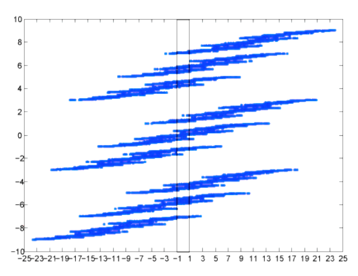Observe now that $x^{\prime}(k),x^{\prime\prime}(k)$ give rise to the same output if and only if the couple $[x^{\prime}(k),x^{\prime\prime}(k)]\in\mathbb{R}^{2}$ belongs to the set (see figure 1)

 
Therefore, if there exist two orbits $\{x^{\prime}(k)\}_{k=1}^{K},\{x^{\prime\prime}(k)\}_{k=1}^{K}$ of the system (1) such that the couple $[x^{\prime}(k),x^{\prime\prime}(k)]\in\mathbb{R}^{2}$ remains in $Q$, then the system (1) is not left invertible. For many reasons (mainly due to the “complexity” of the shape of the set $Q$) it is much easier to check the existence of a sequence of pair of states in $Q_{0}$, the “strip” that includes $Q$ (see figure 1):

 
The problem is then to deduce the presence of an orbit in $Q$ from the existence of an orbit in $Q_{0}$. We solve this problem with the help of the following remarks:

• $\spadesuit$

  Consider the orbits $\{\overline{x(k)^{\prime}}\}_{k=1}^{K}$, $\{\overline{x(k)^{\prime\prime}}\}_{k=1}^{K}$ of the system (1), obtained respectively with initial conditions $[x(0)^{\prime}+\overline{x},x(0)^{\prime\prime}+\overline{x}]$ instead of $[x(0)^{\prime},x(0)^{\prime\prime}]$. Then easy calculations shows that each $[\overline{x(k)^{\prime}},\overline{x(k)^{\prime\prime}}]$ differs from $[x(k)^{\prime},x(k)^{\prime\prime}]$ by a translation along a parallel of the bisecting line of $\mathbb{R}^{2}$.

• $\clubsuit$

  The length of the translation of the state $[\overline{x(k)^{\prime}},\overline{x(k)^{\prime\prime}}]$, up to a constant, is proportional to $a^{k}$, since

  $$\overline{x(k)^{\prime}}=a^{k}(x(0)^{\prime}+\overline{x})+\hbox{terms that depend only on the sequence of u's.}$$

  The same holds for $\overline{x(k)^{\prime\prime}}$.

Therefore the question is the following. Consider an orbit $\Big\{[x(k)^{\prime},x(k)^{\prime\prime}]\Big\}$ which is included in $Q_{0}$. Does there exist a suitable translation $[\overline{x},\overline{x}]$ of the initial states $[x(0)^{\prime},x(0)^{\prime\prime}]$ such that the resulting orbit is indeed in $Q$?

By $\spadesuit$, as $\overline{x}$ varies in $\mathbb{R}$, the initial condition is moving along a parallel of the bisector of $\mathbb{R}^{2}$, but every time it cover a distance of $\sqrt{2}$, it is in the same relative position with respect to a square of $Q$: in other words the property of “being inside $Q$” is periodic.

Moreover, by $\clubsuit$, the distance covered by $[\overline{x(k)^{\prime}},\overline{x(k)^{\prime\prime}}]$ with respect to $[x(k)^{\prime},x(k)^{\prime\prime}]$ is proportional to $a^{k}$, and easy calculations shows that the property of “being inside $Q$”, which is periodic, depends on the fractional parts of $a^{k}$ (see also figure 2).

The Theorem (see also Theorem 5) indeed assures that there exists a suitable translation $[\overline{x},\overline{x}]$ of the initial states $[x(0)^{\prime},x(0)^{\prime\prime}]$ such that the resulting orbit is inside $Q$. Referring to figure 3, each arrow represents the “period” $1$ (in terms of fractional parts, to be multiplied by $\sqrt{2}$), and in particular, the values of fractional parts going from $0$ to the intersection of the square with the arrow correspond to a point inside $Q$. Therefore arbitrary small fractional parts, whose existence is assured by the Theorem, means that every point of the orbit can be positioned inside $Q$ simply modifying the initial conditions in the way we showed. Indeed it is well known also that the numbers $a\in\mathbb{R}$ such that $1,a,a^{2},\ldots,a^{K}$ are linearly independent over $\mathbb{Z}$ are a set of full measure.

That’s the point of this paper. In this work we solve the problem of checking the left invertibility of a system in arbitrary dimension, by investigating the presence of an orbit in the “strip” $Q_{0}$, and then deducing the presence of an orbit in $Q$. This strategy works for a full measure set of parameters.

Throughout this paper we use the following notations:

• •

  $\pi_{p}$ is the canonical projection on the first $p$ coordinates;

• •

  $\pi_{W}$ is the canonical projection on a subspace $W$;

• •

  $\varpi_{i}:\mathbb{R}^{d}\rightarrow\mathbb{R}$ denotes the orthogonal projection on the $i$-th coordinate;

• •

  $e_{i}$ is the $i-$th vector of the canonical basis of $\mathbb{R}^{d}$;

• •

  $\lfloor\cdot\rfloor$ is the floor function, acting componentwise;

• •

  $frac(\cdot)$ denotes the fractional part, acting componentwise;

• •

  $\langle v_{1},\ldots,v_{i}\rangle$ denotes the linear subspace generated by the vectors $v_{1},\ldots,v_{i}$;

• •

  $\mu(S)$ denotes the Lebesgue measure of a set $S$ in $\mathbb{R}^{d}$;

• •

  $\partial$ indicates “topological boundary of …”;

• •

  $\setminus$ denotes the set difference;

• •

  $\mathbb{Q}[\zeta_{1},\ldots,\zeta_{N}]$ is the ring of polynomial in the variables $\zeta_{1},\ldots,\zeta_{N}$, with coefficients in $\mathbb{Q}$;

We consider systems of the form

where $A\in\mathbb{R}^{d\times d},B\in\mathbb{R}^{m\times d},C\in\mathbb{R}^{p\times d}$, $x(k)\in\mathbb{R}^{d}$ is the state, $y(k)\in\mathbb{Z}^{p}$ is the output, and $u(k)\in\mathcal{U}\subset\mathbb{R}^{m}$ is the input. The map $q:\mathbb{R}^{p}\rightarrow\mathbb{Z}^{p}$ is induced by the uniform partition $\mathcal{P}=\bigcup_{i\in\mathbb{Z}^{p}}\mathcal{P}_{i}$ of $\mathbb{R}^{p}$ of rate $\delta$ through $q:(x\in\mathcal{P}_{i})\mapsto i$ and will be referred to as the output quantizer. We assume that $\mathcal{U}$ is a finite set of cardinality $n$.

So we consider only systems of the form

For a ULI system, it is possible to recover the input string until instant $m$ observing the output string until instant $m+k$. For applications, it is important to obtain an algorithm to reconstruct the input symbol used at time $m>l$ by processing the output symbols from time $m$ to $m+k$.

To address left invertibility, we are interested in the following system on $\mathbb{R}^{2d}$:

If there exist sequences $\{u(k)\},\{u^{\prime}(k)\}$, and an initial state in $Q$ such that the corresponding orbit of (4) remains in $Q$, then the two strings of inputs generate the same output for the system (3). So conditions ensuring that the state is outside $Q$ for some $k$ will be investigated to guarantee left invertibility.

In this section we recall some results coming from Iterated Function System theory (see [3, 13] for general theory about IFS), in connection with the notions of left invertibility.

Consider now an output-quantized linear system, together with two sets, namely $\mathcal{H}$ and $S$: $\mathcal{H}$ plays the role of an attractive and invariant set, in which the dynamic of the system is confined, and $S$ plays the role of a quantization set, i.e. a set that the state has to exit to guarantee an invertibility property. In [11] a necessary and sufficient condition for left invertibility of joint contractive systems is given, but here we state the same condition in a more abstract setting: $\mathcal{H}$ and $S$ are an attractor and a quantization set, not the attractor and the quantization set of the system (3). That’s because in the following we will use these results for another attractor and quantization set, i.e. those ones of the difference systems.

If instead the system (3) is joint expansive, then the map $x(k)\mapsto x(k+1)$ admits an inverse for every $u\in\mathcal{U}$. Therefore it is possible to define a correspondent inverse system:

In the case of joint contractive systems, the inverse systems give rise to attractors, since they are joint contractive: such attractors can be described also as the set of initial conditions that can start a bounded orbit of the system (3) or of the doubled system (4):

The first main result is based on a density theorem of Kronecker.

Considering the difference system (Definition 11), we are interested in orbits completely included in $(]-1,1[)^{p}\times\langle e_{p+1},\ldots,e_{d}\rangle.$ The following proposition shows that under a very weak condition orbits completely included in $(]-1,1[)^{p}\times\langle e_{p+1},\ldots,e_{d}\rangle$ must be bounded.

Proof: See Appendix. $\diamondsuit$ 

Note that the set of matrices $A\in\mathbb{R}^{d\times d}$ that have an invariant subspace in $\langle e_{p+1},\ldots,e_{d}\rangle$ is a zero measure set. Define now $\mathbb{S}_{D}(B,\mathcal{U})$ to be the set of matrices $A\in\mathbb{R}^{d\times d}$ such that the system (3) is uniformly left D-invertible, and $\mathbb{S}(B,\mathcal{U})$ to be the set of matrices $A\in\mathbb{R}^{d\times d}$ such that the system (3) uniformly left invertible.

Proof: See appendix. $\diamondsuit$

Linear systems of dimension $1$ assume the following form, deriving from (3):

This is a contractive system if $|a|<1$ and an expansive system if $|a|>1$. If $|a|<1$ the invertibility problem can be solved with the methods of section $3$ (see [10]). The next Theorem shows a necessary condition for the ULI of a system of type (6): if it is not satisfied we construct inductively a pair of strings that gives rise to the same output.

Proof: We will consider sequences of sets of type

where $u(i),u^{\prime}(i)\in\{u_{1},u_{2}\}$ and $\mathcal{P}(i+1)\in\mathcal{P}$ is chosen at each step to maximize the measure of $S_{i+1}$.

In the sequence (7) set $u(1)=u_{1}$, $u^{\prime}(1)=u_{2}$. Since $|u_{1}-u_{2}|<a$, there exists a $\mathcal{P}(1)\in\mathcal{P}$ such that $\mu(S_{1})>0$ (recall that $\mu$ indicates the Lebesgue measure). Then, for $i>1$ define

Since $|a|>2$ there exists an $i_{0}$ such that $\mu\left(S_{i_{0}}\right)=1$, therefore, applying again $u(i_{0}+1)=u_{1}$ and $u^{\prime}(i_{0}+1)=u_{2}$

So there exists $x_{0},x^{\prime}_{0}\in\mathbb{R}$ and $(u(1),\ldots,u(i_{0}+1)),(u^{\prime}(1),\ldots,u^{\prime}(i_{0}+1)),$ with $u(1)\not=u^{\prime}(1)$ and $u(i_{0}+1)\not=u^{\prime}(i_{0}+1)$, such that for the corresponding outputs it holds

It is then enough to point out that, since we can achieve every pair of states $x,x^{\prime}\in S_{i_{0}}$ in the above described way, we can again go on in the same way and find a new instant $i_{1}$, a pair of initial states $x_{1,0},x^{\prime}_{1,0}$, and control sequences $(u(1),\ldots,u(i_{1})),\ (u^{\prime}(1),\ldots,u^{\prime}(i_{1}))$, with $u(i_{1})\not=u^{\prime}(i_{1})$, such that for the corresponding output it holds

Finally, we can achieve by induction an increasing finite sequence, but arbitrarily long, of instants $i_{k}$, pairs of initial states $(x_{k,0},x^{\prime}_{k,0})$, and sequences of controls $(u(1),...,u(i_{k})),(u^{\prime}(1),...,u^{\prime}(i_{k}))$ with $u(i)\not=u^{\prime}(i)$ if $i=i_{j}+1$ for $j=1,...,k-1$ such that such that for the corresponding output it holds

This contradicts the uniform left invertibility property. $\diamondsuit$

The following Theorem can be deduced from Theorem 6, observing that an algebraically independent set of one element is a trascendental number.

Proof: A sufficient condition for uniform left D-invertibility in one step is

indeed in this hypothesis $\forall v\in\mathcal{V},v\not=0$

We now prove that if $\exists v\in\mathcal{V},v\not=0:\ |v|<|a|+1$, then the system is not uniformly left D-invertible. Indeed in this case the system

has the solution $x_{1}=\frac{-v}{a+1},x_{2}=\frac{v}{a+1}$. Since $|x_{1}|,|x_{2}|<1$ the difference system has the infinite orbit $\{x_{1},x_{2},x_{1},x_{2},\ldots\}\subset(]-1,1[)^{p}\times\langle e_{p+1},\ldots,e_{d}\rangle$. Therefore system (6) is not left D-invertible. $\diamondsuit$

Consider the system (3). As stated in Theorem 6, if the elements of the matrix $A$ forms an algebraically independent set, then uniform left D-invertibility is equivalent to uniform left invertibility. A standard method to construct algebraically independent sets can be easily deduced from the following Theorem of Lindemann and Weierstrass:

References

- [1] Artin M, (1991) Algebra. Prentice-Hall
- [2] Baker A, (1993) Trascendental number theory. Camb Univ Press
- [3] Barnsley M, (1993) Fractals everywhere. Acad Press inc
- [4] Bicchi A, Marigo A, Piccoli B, (1992) On the reachability of quantized control sytems. IEEE Trans Autom Control 47(4):546-563
- [5] Bobylev N A, Emel’yanov S V, Korovin S K, (2000) Attractor of discrete controlled systems in metric spaces. Comput Math Model 11(4):321-326
- [6] Brockett R W, Mesarovic M D, (1965) The reproducibility of multivariable control systems. J Math Anal Appl 11:548-563
- [7] Carli R, Fagnani F,Speranzon A,Zampieri S, (2008) Communication constraints in the average consensus problem. Automatica 44:671-684
- [8] Chitour Y, Piccoli B ,(2001) Controllability for discrete systems with a finite control set. Math Control Signal Syst 14:173-193
- [9] Delchamps D F, (1990) Stabilizing a linear system with quantized state feedback. IEEE Trans Autom Control 35(8):916-924
- [10] Dubbini N, Piccoli B, Bicchi A, (2008) Left invertibility of discrete systems with finite inputs and quantized output. Proc 47th IEEE Conf Decis Control 4687–4692
- [11] Dubbini N, Piccoli B, Bicchi A, (2010) Left invertibility of discrete systems with finite inputs and quantised output. Int J Control, 83(4) 798–809
- [12] Edelmayer A, Bokor J, Szabó Z, Szigeti F, (2004) Input reconstruction by means of system inversion: a geometric approach to fault detection and isolation in nonlinear systems. Int J Appl Math Comput Sci 14(2):189-199
- [13] Falconer K, (2003) Fractal geometry, mathematical foundations and applications. John Wiley and Sons
- [14] Gwozdz-Lukawska G, Jachymski J (2005) The Hutchinson-Barnsely theory for infinite interated function systems. Bull Aust Math Soc 72:441-454
- [15] Inoue E, Ushio T, (2001) Chaos communication using unknown input observer. Electron Commun Jpn pt 3 84(12):21-27
- [16] Hardy G H, Wright E M, (1979) An introduction to the theory of numbers. Oxf Sci Publ
- [17] Massey J L, Sain M K, (1969) Invertibility of linear time-invariant dynamical systems. IEEE Trans Autom Control, AC-14(2)141-149
- [18] Massey J L, Sain M K, (1968) Inverses of linear sequential circuits. IEEE Trans Computers C-17:330-337
- [19] Morse A S, Wonham W M, (1971) Status of noninteracting control. IEEE Trans Automat Control, 16(6):568-581
- [20] Picasso B, Bicchi A, (2007) On the stabilization of linear systems under assigned I/O quantization. IEEE Trans Autom Control 52(10):1994-2000
- [21] Respondek W (1990) Right and Left Invertibility of Nonlinear Control Systems. In: Sussmann (ed) Nonlinear Controllability and Optimal Control, NY pp 133-176
- [22] Silverman L M, (1969) Inversion of multivariable linear systems. IEEE Trans Automat Control 14(3):270-276
- [23] Sontag E D, (1998) Mathematical control theory: deterministic finite dimensional systems. Springer, NY
- [24] Szanier M, Sideris A, (1994) Feedback control of quantized constrained systems with applications to neuromorphic controller design. IEEE Trans Autom Control 39(7):1497-1502
- [25] Tanwani A, Liberzon D, (2010) Invertibility of switched nonlinear systems. Automatica, 46:1962-1973
- [26] Tatikonda S C, Mitter S, (2004) Control under communication constraints. IEEE Trans Autom Control 49(7):1056-1068
- [27] van Schuppen J H, (2004) Decentralized control with communication between controllers. In: Blondel V D, Megretski A (ed) Princet Univ Press, Princeton, pp 144–150
- [28] Vu L, Liberzon D, (2008) Invertibility of switched linear systems. Automatica, 44:949-958