Explosive Percolation is Continuous, but with Unusual Finite Size Behavior
Abstract
We study four Achlioptas type processes with “explosive” percolation transitions. All transitions are clearly continuous, but their finite size scaling functions are not entire holomorphic. The distributions of the order parameter, the relative size of the largest cluster, are double-humped. But – in contrast to first order phase transitions – the distance between the two peaks decreases with system size as with . We find different positive values of (defined via for infinite systems) for each model, showing that they are all in different universality classes. In contrast, the exponent (defined such that observables are homogeneous functions of ) is close to – or even equal to – 1/2 for all models.
pacs
64.60.ah, 05.70.Jk, 89.75.Da, 05.40.-aPercolation is a pervasive concept in statistical physics and probability theory and has been studied in extenso in the past. It came thus as a surprise to many, when Achlioptas et al. [1] claimed that a seemingly mild modification of standard percolation models leads to a discontinuous phase transition – named “explosive percolation” (EP) by them – in contrast to the continuous phase transition seen in ordinary percolation. Following [1] there appeared a flood of papers [2, 3, 5, 5, 6, 7, 8, 9, 10, 11, 12, 4, 14, 15, 16, 17, 18, 19, 2] studying various aspects and generalizations of EP. In all cases, with one exception [2], the authors agreed that the transition is discontinuous: the “order parameter”, defined as the fraction of vertices/sites in the largest cluster, makes a discrete jump at the percolation transition. In the present paper we join the dissenting minority and add further convincing evidence that the EP transition is continuous in all models, but with unusual finite size behavior.
From the physical point of view, the model seems somewhat unnatural, since it involves non-local control (there is a ‘supervisor’ who has to compare distant pairs of nodes to chose the actual bonds to be established 11 1 In contrast to claims made by the authors, the model in [7] is also non-local by any standard physics definition.). Also, notwithstanding [8], no realistic applications have been proposed. It is well known that the usual concept of universality classes in critical phenomena is invalidated by the presence of long range interactions. Thus it is not surprising that a percolation model with global control can show completely different behavior [22].
Usually, e.g. in thermal equilibrium systems, discontinuous phase transitions are identified with “first order” transitions, while continuous transitions are called “second order”. This notation is also often applied to percolative transitions. But EP lacks most attributes – except possibly for the discontinuous order parameter jump – considered essential for first order transitions. None of these other attributes (cooperativity, phase coexistence, and nucleation) is observed in Achlioptas type processes, although they are observed in other percolation-type transitions [23]. Thus EP should never have been viewed as a first order transition, and it is gratifying that it is also not discontinuous.
Apart from the behavior of the average value of the order parameter , phase transitions can also be characterized by the distribution of in finite systems, where is the control parameter and measures the system size. For infinite , jumps at if the transition is discontinuous, while it varies continuously with a power law singularity for a continuous transition. The distribution at criticality scales, for continuous transitions, as [24]
| (1) |
where for standard thermal second order phase transitions. The universal function might be double-humped, as in the Ising model [24]. But then, as , the dip between the humps usually does not deepen and the horizontal distance between them shrinks to zero so that becomes single-humped.
Equation (1) is directly related to the finite size scaling (FSS) of [25],
| (2) |
where the universal scaling function is analytic at all finite , reflecting the fact that the critical point was the only singularity of the partition function, before it was regularized by Eq.(2). Notice that the usual FSS ansatz [25] involves the linear system size instead of with , where is the dimension and is the correlation length exponent.
In typical first order transitions, in contrast, is double-humped with a deepening valley between the two peaks. The distance between the peaks tends to a positive constant which is equal to the jump in . The depth of the valley between the peaks reflects the fact that values of between the peaks correspond to systems with two co-existing phases and an interface between them that costs energy and is disfavored. As a consequence, systems with first order transitions typically do not show FSS (unless the interface energy does not increase with system size [26]).


In percolation, usually the relative size of the largest cluster, , is taken as an order parameter. Here, is the number of nodes, and for and . In [6, 16] it was observed that is strongly double-peaked in EP transitions. In [16] this was also backed by careful measurements of the depth of the valley between the peaks, which indeed lowered with increasing . This was taken as a clear indication for the transition being first order and for phase coexistence. Notice that the latter is not justified since is, in contrast to the local order parameters in thermal systems, a global quantity and cannot be used to characterize any part of a large system. Rather, the structure of in EP reflects the suddenness of the transition, combined with a scatter of the precise -values where individual systems acquire giant clusters. At -values where both peaks have the same height, it is much more likely to find either no giant cluster or a fully developed one, than to find a half-grown giant cluster. Hence, the two peaks are more reminiscent of systems without self-averaging [27] than of phase coexistence.
While the two peaks prove the suddenness of the transition that was claimed as a hallmark of EP, they do not yet prove that EP is discontinuous. For that, one must also show that the distance between the peaks does not vanish for . In order to check this, we have made extensive simulations of four models: The original product rule of [1], denoted in the following as “PR”; The product rule on 2-d square lattices [3, 5] with helical boundary conditions (“2d”); The ‘adjacent edge’ rule [7] (“AE”); And the rule of [2] (“da Costa”). For more details on the simulations, see the supplementary material (SM).
| PR | 2d | AE | da Costa | |
|---|---|---|---|---|
| 0.888449(2) | 0.526562(3) | 0.797013(3) | 0.923207508 | |
| 0.0402(15) | 0.018(2) | 0.103(2) | 0.0255(8) | |
| 0.270(7) | 0.078(7) | 0.228(5) | 0.300(5) | |
| 0.0861(5) | 0.040(2) | 0.214(2) | 0.0557(5) | |
| 0.47(2) | 0.45(6) | 0.48(1) | 0.46(2) | |
| 0.52(1) | 0.47(3) | 0.51(1) | 0.53(1) | |
| 1/2 | – | 1/2 | 1/2 | |
| 0.0567(9) | 0.0612(8) | 0.1113(8) | 0.0356(8) |


Distributions for these models are shown in Fig. 1. In all cases was chosen such that both peaks have equal height (set arbitrarily to 1). The extrapolations of these values for are given in Table 1. They agree within errors with the critical values quoted in the literature. We see that in each case the valley between the peaks deepens with increasing [16], but at the same time both peaks shift to the left. Among the three off-lattice models, the AE model (the least non-local) shows the fastest peak shifting and slowest valley deepening, while the opposite is true for the da Costa model. In all cases this shift is compatible with power laws
| (3) |
where is the position of the right (left) peak at the critical point. In all cases (see Table 1), i.e. the right peak moves slower than the left one. Therefore the distance between the peaks increases for small , but has finally to decrease . Since this distance is asymptotically proportional to the maximum of the variance of 22 2 Here we use the observation [16] that the peaks mainly change their heights when is changed, and stay approximately at the same position – the slight shifts of their positions during this change might indeed be responsible for the differences between and . , we find that the variances first increase with (in agreement with [5]), but ultimately must decrease.
As shown in Fig. 2 for the da Costa model, not only the positions of the peaks scale, but also their widths. This indicates that the asymptotic scenario is two well separated peaks with independent shapes whose widths are proportional to their positions. If we switch from defining by equal peak heights to equal peak areas [28] and allow weak convergence for (in contrast to the usual assumption of pointwise convergence; see SM) the full distributions at then show asymptotic scaling
| (4) |
with the scaling function consisting of a finite width right hand peak and a peak at .

For strictly larger than , only the right hand peak dominates the average . We then expect only small finite size scaling corrections to its asymptotic values, i.e. we expect the curves for different to coincide for on a common curve . Since the scenario in this regime is not much different from other critical phenomena this should be a power law that holds in the range . Measured values of are given in Table 1. For the da Costa model the agreement with [2] is perfect. Assuming Eq. (2), it follows that . Values of obtained from this, denoted as , are slightly smaller than 1/2 for all models (see Table 1).
Deviations from this common power law are expected to set in when decreases below . The data for the da Costa model are shown in Figs. 3. For all (except for very small values of ), these deviations are fully described by the FSS ansatz in Eq. (2). In Figs. 3 we chose so that the collapse is best at , resulting in the value quoted in Table 1. For the other models the data collapse is similarly good, except for the 2d model where it is worse (see SM). For all models, is slightly larger than .
The fact that in Eq. (4) contains a -peak at its leftmost extremity implies that in Eq.(2) must vanish for all below some value , which in turn means that must have a singularity at . Indeed, Fig. 4 shows that the values of for approach 0 very fast with increasing , implying (the latter is also true for the other models). We cannot exclude the possibility the curves in Fig. 4 approach a pure power law (dashed red line) in the limit .
The blow-up of the region around shown in the inset in Fig. 4 hints at a power law with (see also SM). The same is qualitatively true for the other models, where always (see Table 1). We see therefore that is no longer in the realm of uniform pointwise convergence to the FSS ansatz, and that therefore . We should finally mention that we used in Fig. 4, a value in between and , as it gives the most systematic behavior for . The same is true the other off-lattice models (but not for the 2d model, see SM), whence we conjecture that for them.
The singularity of at implies also that one cannot expect the effective critical points to scale as . Results obtained for the da Costa model, with defined via equal peak masses, are shown in the SM. They indicate that with . The agreement with the prediction of [2] – based on “standard scaling relations” – seems fortitious.
In this paper we do not present a detailed theory for the convergence to for , in particular we do not explain how and are related to the exponent . It could be that such a theory can be formulated more easily using either or as an order parameter. But this would be beyond the scope of the present paper.

In summary, we have shown that at least four models of explosive percolation, including the original product rule of Achlioptas et al. [1], have continuous transitions. Each is in a different universality class, but all of them show unusual finite size behavior with a non-analytic scaling function. They all show double-peaked order parameter distributions with the sharpness of the peaks increasing with system size, and different scaling laws for the width of the scaling region ( ) and for the shift of the effective . It would be interesting to see whether similar scaling holds in other percolation models with supposedly discontinuous transitions that are not explicitly related to Achlioptas-like dynamics [9, 14, 29]. It could be that the features found in the present paper arise from the specific non-locality of the Achlioptas process, and that this is why it was not seen previously in other critical phenomena.
We are indebted to Bob Ziff and Liang Tian for most useful correspondence.
References
- [1] D. Achlioptas, R. M. D’Souza, and J. Spencer, Science 323, 1453 (2009)
- [2] E. J. Friedman and A. S. Landsberg, Phys. Rev. Lett. 103, 255701 (2010)
- [3] R. M. Ziff, Phys. Rev. Lett. 103 (2009)
- [4] R. M. Ziff, Phys. Rev. E 82, 051105 (2010)
- [5] F. Radicchi and S. Fortunato, Phys. Rev. Lett. 103, 168701 (2009)
- [6] F. Radicchi and S. Fortunato, Phys. Rev. E 81, 036110 (2010)
- [7] R. M. D’Souza and M. Mitzenmacher, Phys. Rev. Lett. 104, 195702 (2010)
- [8] H. D. Rozenfeld, L. K. Gallos, and H. A. Makse, Eur. Phys. J. B 75, 305 (2010)
- [9] S. S. Manna and A. Chatterjee, e-print arXiv:0911.4674(2009)
- [10] A. A. Moreira et al., Phys. Rev. E 81, 040101 (2010)
- [11] Y. S. Cho, B. Kahng, and D. Kim, Phys. Rev. E 81, 030103 (2010)
- [12] Y. S. Cho et al., Phys. Rev. Lett. 103, 135702 (2009)
- [13] Y. S. Cho et al., Phys. Rev. E 82, 042102 (2010)
- [14] N. A. M. Araújo and H. J. Herrmann, Phys. Rev. Lett. 105, 035701 (2010)
- [15] U. Basu et al., e-print arXiv:1008.4293(2010)
- [16] L. Tian and D.-N. Shi, e-print arXiv:1010.5990(2010)
- [17] W. Chen and R. M. D’Souza, e-print arXiv:1011.5854(2010)
- [18] J. Nagler, A. Levina, and M. Timme, Nature Physics, NPHYS1860(2011)
- [19] H. Hooyberghs and B. Van Schaeybroeck, e-print arXiv:1102.0734(2011)
- [20] R. A. da Costa et al., Phys. Rev. Lett. 105, 255701 (2010)
- [21] In contrast to claims made by the authors, the model in [7] is also non-local by any standard physics definition.
- [22] C. Christensen et al., e-print arXiv:1012.1070(2010)
- [23] H.-K. Janssen, M. Müller, and O. Stenull, Phys. Rev. E 70, 026114 (2004)
- [24] A. D. Bruce and N. B. Wilding, Phys. Rev. Lett. 68, 193 (1992)
- [25] K. Binder and D. W. Heermann, Monte Carlo Simulations in Statistical Physics, 5th edition (Springer, Heidelberg, 2010)
- [26] M. S. Causo, B. Coluzzi, and P. Grassberger, Phys. Rev. E 62, 3958 (2000)
- [27] S. Wiseman and E. Domany, Phys. Rev. Lett. 81, 22 (1998)
- [28] Here we use the observation [16] that the peaks mainly change their heights when is changed, and stay approximately at the same position – the slight shifts of their positions during this change might indeed be responsible for the differences between and .
- [29] S. V. Buldyrev et al., Nature 464, 1025 (2010)
Supplementary Material for “Explosive Percolation is Continuous, but with Unusual Finite Size Behavior”
I Simulation Details
All simulations reported in the paper were made using modified versions of the fast Newman-Ziff algorithm [1], on a Linux workstation cluster. System sizes varied between and ( is the number of nodes). For the smaller systems realizations were made for each model, and for the largest systems this number was still . The control parameter is defined as in the references where the 4 models were introduced, as where is the number of links.
Data were actually collected for fixed , where is the number of clusters – more precisely, in order to reduce the data files, was binned (typically with for smallest and for largest ). The values of quoted in the paper are average values over these bins. Since most clusters in all four models are trees, except when is very large, there are very small fluctuations of for fixed , and depends smoothly on . Moreover, test runs showed that the dependence of on is at least as crisp as the dependence on , i.e. is actually the more relevant control parameter.
Mass distributions (Figs. 1 and 2 in the main paper) are obtained by binning, with typically 200 to 500 bins, and with bin sizes slowly increasing with in order to take into account that the left hand peaks in Fig. 1 are sharper than the right hand peaks. For small the distributions shown in Figs. 1 and 2 are the raw data, modified just by interpolating between neighboring bins to obtain exactly equally high peaks (usually, no bin will have two peaks which have exactly equal height; by “interpolating” we mean taking weighted linear averages of the two histograms) and by normalizing them. For the largest this would have given too noisy plots, and cubic splines were used to make the plots more smooth.
Unless otherwise noted, values are those in Table 1. They were determined by having best power laws for at .
II Modified Finite Size Scaling
The finite size scaling ansaetze Eqs. (1) and (2) are of course never exact, and are usually understood as
| (1) |
and
| (2) |
for any fixed finite value of . The limits here are pointwise limits, i.e. the norms of the differences between left and right hands converge uniformly to zero in any finite interval of . Furthermore, and are usually analytic (holomorphic) for all finite .
In a typical first order (discontinuous) transition, an attempt to construct would give a function with two -peaks. In that case the convergence could at best be weak, i.e. in distribution sense. Usually one prefers to call this not finite size scaling at all, although this is strictly spoken a matter of taste and convention.
In explosive percolation one has a “mixed” situation: For the right hand peaks in Figs. 1 and 2 of the main paper one has pointwise convergence, if one chooses . But then the left hand peak converges to a -peak, i.e. the entire function is approached only in the weak sense. Similarly, for the convergence is strong (and is analytic) for (strict inequality!), where only the right hand peak of contributes. The function must vanish identically when only the left (-) peak contributes, which means that it must have a singularity at , and convergence can only be weak in any interval containing . As for first order transitions, it is a matter of convention whether one calls this finite size scaling at all (as we did in this paper).
III Analoga to Fig. 3 (main paper) for the other three models
In the main paper, we showed in Fig. 3 for the da Costa model how scales for , and we said that a data collapse similar to that shown in the inset holds also for the other two off-lattice models, while the collapse is much worse for the 2d model. We now show these data in Figs. S1 to S3.


IV Various other plots for the da Costa model
Although the scaling behavior of the order parameter with at can, in principle, be inferred from Fig. 4 (main paper), we show the data also explicitly in Fig. S4. In this figure we use three possible values of (one of them being the value obtained in [2], in order to show how strongly the exponent depends on .

Results for , the effective critical points on finite systems, are given in Fig. S5. Notice that values of depend crucially on the operational procedure used to define effective critical points. One possibility would be e.g. the point where the two peaks in have equal height (Fig. 1). For the da Costa model, this would give non-monotonic dependence on . More natural seems the definition via equal areas under the two peaks. Notice that this would give ambiguous results for the 2d and AE models, as there the dips between the peaks are not very deep. But for the da Costa model this is unproblematic. Figure 5 shows that our best estimate of is slightly below the value of [2], giving thereby the largest contribution to the uncertainty of the exponent (this slight inconsistency is also the reason why we used also these smaller values in Fig. S4).

Alternatively, we could define as the point where has maximal variance. Variances of are plotted in Fig. S6 against . We see distributions which are for small markedly skewed and shifted away from the origin, but which become increasingly symmetric and centered at the origin as increases. Although this gives a much less precise estimate of than Fig. S5, it demonstrates also that .

Plots similar to Figs. S5 and S6 were not made for the other models, the main reason being the larger uncertainties of .
V For the 2d model, is strictly smaller than 1/2
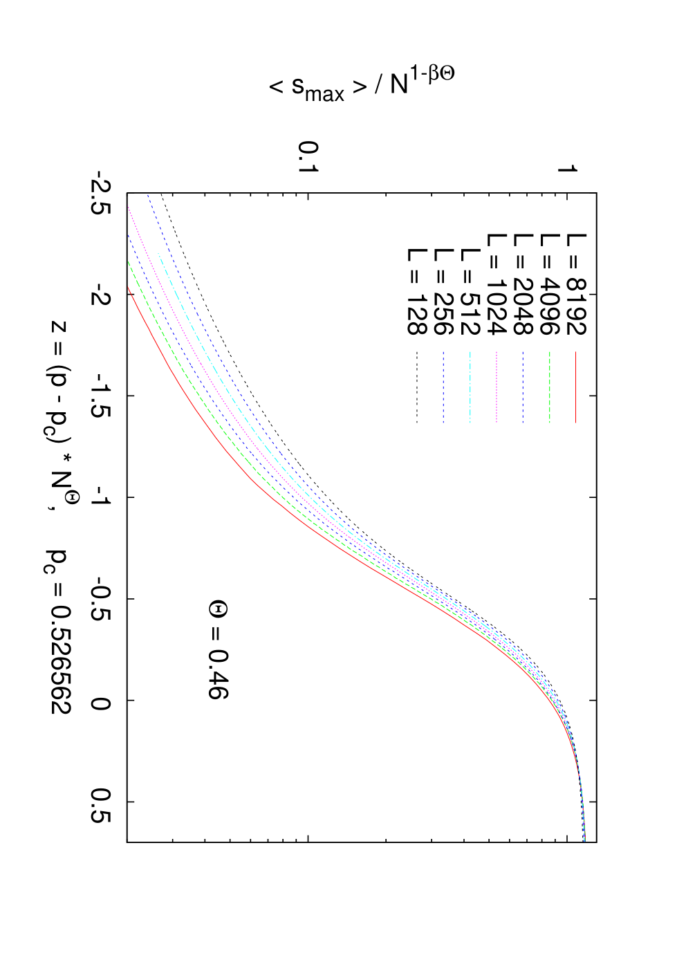
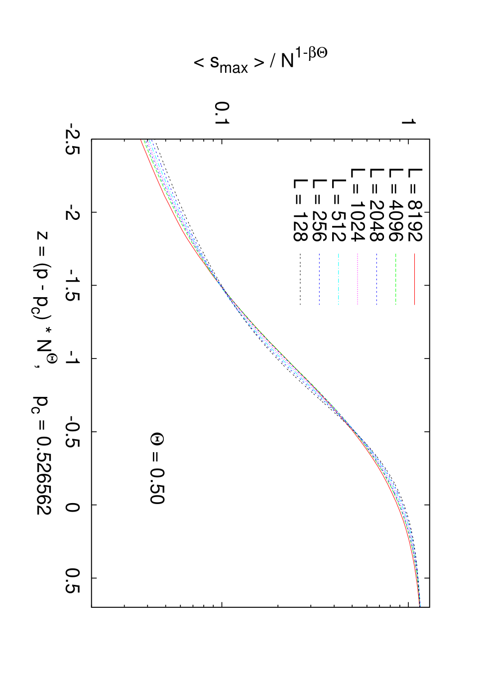
As we said in the paper, one observation that corroborates for the off-lattice models is that it gives very “regular” behavior of in the near subcritical region. Instead of showing here the evidence for this, we show for the 2d model what can go wrong, if is chosen badly. More precisely, we show in the top panel of Fig. S7 results for , and results for in the lower panel. It seems clear that panel (b) is not very plausible, in particular since the scaling with of the left hand peaks in Fig. 1 requires that the curves decrease with for . For the other models similar curve crossings appeared when was used instead of .
VI Further comparisons with previous papers
a) To our knowledge, the only previous work where was seen in a continuous phase transition is [3]. This dealt with interacting self avoiding walks in 4 dimensions. The authors also found double-peaked distributions of the order parameter, but they did not report different scaling laws for both peaks. Thus the reason for was not explained, as in our case, via a singularity of the scaling function . Also, in [3] the authors found , while we found in our models .
b) A different scaling theory for the PR model was presented in [4]. The authors there started from the assumption that is independent of at , which is definitely not true for any of the four models according to our simulations. Although this prevents our theories from being equivalent, there are some similarities. In particular, the authors of [4] show that the width of the FSS region scales as with , which is very close to our conjectured value .
c) A detailed study of the 2d model was made in [5]. The most remarkable agreement is that was measured there as , while we found . The slight discrepancy is partially due to a slightly different estimate of ( in [5] against in the present work). Also the estimate of the Fisher exponent in [5] is fully compatible with our value of , if we accept the relationship between the two exponents given in [2].
References
- [1] M. E. J. Newman and R. M. Ziff, Phys. Rev. E 64, 016706 (2001)
- [2] R. A. da Costa et al., Phys. Rev. Lett. 105, 255701 (2010)
- [3] T. Prellberg and A. L. Owczarek, Phys. Rev. E 62, 3780 (2000)
- [4] Y. S. Cho et al., Phys. Rev. E 82, 042102 (2010)
- [5] R. M. Ziff, Phys. Rev. E 82, 051105 (2010)