Testing String Vacua in the Lab: From a Hidden CMB to Dark Forces in Flux Compactifications

Preprint: DESY 11-042; IPPP/11/13; DCTP/11/26

Michele Cicoli Email: michele.cicoli@desy.de Affiliation: Theory Group, Deutsches Elektronen-Synchrotron DESY, Notkestrasse 85, D-22607 Hamburg, Germany Mark Goodsell Email: mark.goodsell@desy.de Affiliation: Theory Group, Deutsches Elektronen-Synchrotron DESY, Notkestrasse 85, D-22607 Hamburg, Germany Joerg Jaeckel Email: joerg.jaeckel@durham.ac.uk Affiliation: Institute for Particle Physics Phenomenology, Durham University, Durham DH1 3LE, United Kingdom. Andreas Ringwald Email: andreas.ringwald@desy.de Affiliation: Theory Group, Deutsches Elektronen-Synchrotron DESY, Notkestrasse 85, D-22607 Hamburg, Germany

Abstract:

We perform a detailed analysis of the phenomenological properties of hidden Abelian gauge bosons with a kinetic mixing with the ordinary photon within type IIB flux compactifications. We study the interplay between moduli stabilisation and the Green-Schwarz mechanism that gives mass to the hidden photon paying particular attention to the rôle of $D$ -terms. We present two generic classes of explicit Calabi-Yau examples with an isotropic and an anisotropic shape of the extra dimensions showing how the last case turns out to be very promising to make contact with current experiments. In fact, anisotropic compactifications lead naturally to a GeV-scale hidden photon (“dark forces” that can be searched for in beam dump experiments) for an intermediate string scale; or even to an meV-scale hidden photon (which could lead to a “hidden CMB” and can be tested by light-shining-through-a-wall experiments) in the case of TeV-scale strings.

$e$ -mail: ; ; ;

1 Introduction

Recently there has been quite some interest in the possibility that there exist hidden sector particles with masses below a TeV but very weak couplings to Standard Model matter. They are a common feature of extensions of the standard model based on supergravity or superstrings. Extra $U(1)$ gauge bosons, so-called hidden photons are a prime candidate for such particles. At low energies, their interactions with the visible sector occur primarily via kinetic mixing [1, 2] (studied in string theory in [3, 4, 5, 6, 7, 8, 9, 10, 11, 12, 13]) with the electromagnetic¹¹ 1 Of course, the mixing is originally with the hypercharge $U(1)$ but after electroweak symmetry breaking this mixing is inherited by the electromagnetic $U(1)$ .²² 2 A massive hidden photon behaves very similar to a $Z^{\prime}$ . However, a hidden photon is more specific in the sense that its coupling to Standard Model particles is proportional the ordinary electric charge of a particle and the kinetic mixing parameter $\chi$ which is usually small. As the coupling to Standard Model matter is naturally quite small hidden photons can often be quite light without being in conflict with existing experiments or observations. $U(1)$ ,

\displaystyle\mathcal{L}\supset-\frac{1}{4}F^{({\rm vis})}_{\mu\nu}F^{\mu\nu}_{({\rm vis})}-\frac{1}{4}F^{({\rm hid})}_{\mu\nu}F^{\mu\nu}_{({\rm hid})}+\frac{\chi}{2}F_{\mu\nu}^{({\rm vis})}F^{({\rm hid})\mu\nu}+m_{\gamma^{\prime}}^{2}A^{({\rm hid})}_{\mu}A^{({\rm hid})\mu}+A^{({\rm vis})}_{\mu}j^{\mu},

(1)

where $\chi$ is the kinetic mixing parameter and $m_{\gamma^{\prime}}$ the mass of the hidden $U(1)$ , which may arise via a hidden Higgs or a Stückelberg mechanism. In addition $j^{\mu}$ is the current caused by charged Standard Model matter such as electrons and protons.

There are two mass regimes that are of particular phenomenological interest: the meV range and the GeV range, marked “hCMB” and “Dark Forces” in Fig. 1, respectively. The characteristic behaviour of these two regimes is best understood in slightly different pictures.

At very low masses the most prominent implication of kinetic mixing is that, similar to neutrino mixing, the propagation and the interaction eigenstates are misaligned. As a result one expects photon $\leftrightarrow$ hidden photon oscillations [1]. These oscillations could lead to a variety of interesting phenomena. In the early universe they convert thermal photons into hidden photons, generating a “hidden CMB” (hCMB) [14]. Its signature is an increase in the effective number of relativistic degrees of freedom contributing to the cosmic radiation density in the era between big bang nucleosynthesis and recombination beyond the value accounting for the photon and the three standard neutrino species. Intriguingly, some global cosmological analyses that take into account precision cosmological data of the cosmic microwave background and of the large scale structure of the universe appear to require some extra radiation density. The case for this was strengthened by the recently released WMAP 7 year data whose global analysis points to the requirement of an equivalent of $\Delta N_{\nu}^{\mathrm{eff}}=1.3\pm 0.9$ (68 $\%$ C.L.) neutrinos [15].

Luckily, hidden photons in the meV range can be nicely searched for in purely laboratory based laser-light-shining-through-a-wall experiments [16, 17], such as ALPS [18], BMV [19], GammeV, LIPSS [20], and OSQAR (cf. the bounds marked “LSW” in Fig. 1), with great discovery potential in the near future [21] and even the possibility of long distance communication through matter [22]. The discovery potential is also shared by upcoming microwave cavity experiments [23, 24, 25], which are currently in the pioneering phase [26, 27]. In addition, dedicated helioscope searches, e.g. such as SHIPS at the Hamburg Observatory, for hidden photons produced in the sun could also sensitively explore this region [28].

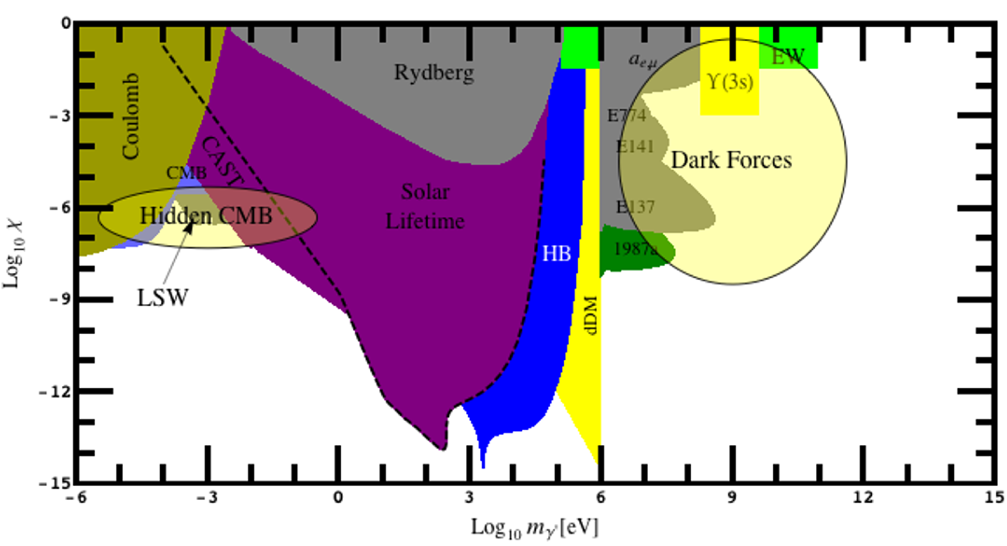
Refer to caption — Figure 1: Constraints on the kinetic mixing parameter $\chi$ vs. hidden photon mass $m_{\gamma^{\prime}}$ from astrophysics, cosmology and laboratory experiments. Phenomenologically interesting regions are marked in yellow. Compilation from [29].

At larger masses $\gtrsim$ MeV a convenient choice of basis is such that charged Standard Model matter acquires a small charge under the extra hidden $U(1)$ leading to a “Dark Forces” interaction. This type of interactions can be used to explain a variety of puzzling observations connected to dark matter and astrophysics, such as the results of DAMA, CoGeNT and PAMELA [30, 31, 32, 33, 34, 35]. Moreover, they provide an interesting explanation for the deviation $(g-2)_{\mu}$ from the Standard Model prediction [36]. These higher masses, too can be sensitively probed in laboratory experiments. A tool of choice are fixed target experiments [37] where a high current beam of electrons or protons impacts on a block of material. A significant number of such experiments are in planning or in trial phases: DESY (HIPS [38]), MAMI [39] and Jefferson Lab (APEX [40], HPS [41] and DarkLight [42]).

Given this great phenomenological interest and the huge discovery potential for hidden photons, it is timely to ask whether there are interesting classes of string compactifications which will lead to kinetic mixing and masses in the ranges described above.

We shall argue that this is indeed the case in a variety of string models based on type IIB flux compactifications on Calabi-Yau orientifolds with $D3$ / $D7$ -branes and $O3$ / $O7$ -planes [8, 10], unlike for example the heterotic case [3, 11] where there is no natural way to suppress the mixing and masses. The hidden photon can be realised as an excitation of a space-time filling $D3$ or a $D7$ -brane wrapping an even 4-cycle in the extra dimension separated from the locus of the $D$ -brane hosting the hypercharge $U(1)$ by distances greater than a string length. This ensures that there are no light states with masses $\lesssim M_{s}$ charged under both the Standard Model and the hidden gauge groups, ensuring that the extra $U(1)$ is indeed “hidden”.

In the $D3$ -brane case the kinetic mixing cannot be much smaller than $\chi\simeq 10^{-3}$ , while if a $D7$ -brane wraps a large 4-cycle $\tau_{hid}$ , giving rise to a tiny gauge coupling $g^{-2}\simeq\tau_{hid}$ , the physical mixing parameter can be significantly suppressed. Therefore we shall focus on hidden photons living on these “milliweak” or “hyperweak” $D7$ -branes. The hidden photon becomes massive via the Green-Schwarz mechanism by turning on a non-zero world-volume flux. Some Kähler moduli get charged under the hidden $U(1)$ and a particular combination of the corresponding axions get eaten up by the hidden photon. We stress that this is a truly stringy mechanism that leads to robust predictions unlike the case of a Higgs mechanism which depends more heavily on the details of the particular brane construction ³³ 3 Moreover, if we aim to generate masses of $\mathcal{O}({\rm meV})$ with a sizeable mixing $\chi\sim 10^{-6}$ , the very stringent constraints on millicharged particles would require an extremely steep hidden Higgs potential in order that their masses would be above a MeV..

The turning on of gauge fluxes also generates a moduli-dependent Fayet-Iliopoulos term whose effect on moduli stabilisation has to be taken into account. One of the most promising ways to fix the geometric moduli in a controlled manner is given by the type IIB LARGE Volume Scenario [43, 44]. We shall embed our models into this moduli stabilisation framework since it does not require fine-tuning of the background fluxes and can generate exponentially large extra dimensions with the subsequent possibility to lower the string scale, $\chi$ and $m_{\gamma^{\prime}}$ .

Ref. [10] studied the properties of hidden photons within the original formulation of the LARGE Volume Scenario where the compactification is isotropic in that the largest two-cycle $t_{big}$ is of the order of the cube root of the volume: $t_{big}\simeq{\cal V}^{1/3}$ , but without analysing the rôle played by $D$ -terms in moduli stabilisation. In this paper we show that $D$ -terms for the hyperweak brane are in general dangerous since they give rise to a run-away for the volume mode. We propose then a solution where $D$ -terms do not cause any decompactification but dynamically reduce more complicated topologies to the ones studied in [10].

The isotropic case leads to nice predictions which however fail to reach the interesting regions of parameter space corresponding to either hidden CMB or dark forces. However, once we consider more involved compactification manifolds with a fibration structure as in [44], the desired masses and mixings can be easily accommodated due to the anisotropic shape of the extra dimensions. In fact, we show that the moduli can be fixed with a single two-cycle that scales as entire volume: $t_{big}\simeq{\cal V}$ . This is complementary to some work in progress [45], which shows how maximally anisotropic extra dimensions can be stabilised. In this case, closed strings propagating along this cycle would be extremely diluted, and would allow vastly smaller masses for $U(1)$ fields that they couple to. In this way, the relationship between kinetic mixing and $U(1)$ masses changes dramatically giving rise to a very interesting phenomenology in the case of “milliweak” $D7$ -branes where we find two scenarios:

•

“Dark force scenario”: the Kähler moduli are stabilised without fine-tuning leading to hidden photons with $m_{\gamma^{\prime}}\simeq 1$ GeV and $\chi\simeq 10^{-6}$ . The string scale turns out to be intermediate and the Calabi-Yau geometry is slightly anisotropic;
•

“Hidden CMB scenario”: fine-tuning the underlying parameters, the stabilisation of the Kähler moduli leads to hidden photons with $m_{\gamma^{\prime}}\simeq 1$ meV and $\chi\simeq 10^{-6}$ . This corresponds to the extreme case of TeV-scale strings and very anisotropic compactification manifolds. Furthermore, Kaluza-Klein replicas of the hidden gauge bosons turn out to be in the dark force mass regime.

This paper is organised as follows: section 2 provides the essential background information on the properties of D-brane $U(1)$ s in IIB compactifications, and establishes our notations; additional description and derivations are presented in the appendix A. In section 3 we describe how anisotropy in IIB compactifications can lead to interesting phenomenology. In section 4 we show how to stabilise the moduli. Section 5 presents our main results; the predictions for scenarios with stable moduli. It is relatively self-contained so a reader interested only in the predictions testable in experiments can skip the interim sections. Finally we conclude in section 6.

2 Abelian gauge bosons in IIB compactifications

In this section we shall summarise the formulae pertaining to Abelian gauge bosons on D-branes in IIB compactifications that we shall require later. While the material here is not new, we hope that the novel presentation will facilitate their use in model building, specifically for models with stabilised moduli. We present additional explanations and derivations for readers unfamiliar with the material in appendix A.

Such models are compactified on a Calabi-Yau threefold $\mathcal{M}_{6}$ which supports a basis of (1,1)-forms $\hat{D}_{i}$ , with Kähler form expanded in terms of these forms $J=t^{i}\hat{D}_{i}$ , intersection numbers

k_{ijk}=\int_{\mathcal{M}_{6}}\hat{D}_{i}\wedge\hat{D}_{j}\wedge\hat{D}_{k},

(2)

and thus the volume of the manifold is $\mathcal{V}=\frac{1}{6}\int J\wedge J\wedge J=\frac{1}{6}k_{ijk}t^{i}t^{j}t^{k}$ . Gauge and matter fields are supported on D7 branes wrapping divisors (four-cycles) on the compact space. There is a canonical basis of four-cycles where the Poincaré dual two-form is a $\{\hat{D}_{i}\}$ ; these have volume $\tau_{i}=\frac{1}{2}k_{ijk}t^{j}t^{k}$ where (neglecting cycles odd under the orientifold) the $\tau_{i}$ are the real part of the good Kähler coordinates for the field theory. A stack of $N$ branes on such a cycle supports a $U(N)$ gauge theory if it is not pointwise invariant under the orientifold projection; if it is then the gauge group is either $Sp(N)$ or $SO(N)$ (depending upon whether the orientifold plane wrapped by the brane is of $O^{+}$ or $O^{-}$ type). For a $U(1)\subset U(N)$ the gauge coupling on a brane wrapping such a cycle is given by

\frac{2\pi}{g_{i}^{2}}=\tau_{i}.

(3)

Importantly if the volume of the four cycle is large the gauge coupling can be weak or even hyperweak [46].

The theory has a classical Kähler potential given by

K_{0}\equiv-2\log\mathcal{V},

(4)

which will be modified in the later sections to include corrections due to finite string length and coupling. The above may also be augmented by contributions from collapsed cycles of volume $\tau_{0}\approx 0$ of the form $\Delta K=c\frac{(\tau_{0})^{2}}{\mathcal{V}}$ . However, derived from the above is the classical Kähler metric for the moduli, given by derivatives with respect to the Kähler coordinates

(\mathcal{K}_{0})_{ij}\equiv\frac{\partial^{2}}{\partial\tau_{i}\partial\tau_{j}}K_{0}.

(5)

2.1 Stückelberg masses

We shall consider only $U(1)$ s supported on D7 branes (rather than R-R $U(1)$ s [47, 11]) since these are generically present in the theory, have the possibility of mixing kinetically with the hypercharge (which must itself be supported on a D7 brane in such models) and crucially may obtain Stückelberg masses. The Stückelberg mass matrix for the $U(1)$ s $a,b$ that do not couple to any cycles odd under the orientifold are given by [48, 49, 50, 10] ⁴⁴ 4 Allowing for cycles odd under the orientifold plane leads to larger masses and thus less interesting phenomenology; nevertheless the full expression is given in appendix equation (149)

\displaystyle m_{ab}^{2}=

\displaystyle g_{a}g_{b}\,\frac{M_{P}^{2}}{4\pi^{2}}q_{a\alpha}(\mathcal{K}_{0})_{\alpha\beta}q_{b\beta},

(6)

where $M_{P}=2.4\times 10^{18}$ GeV is the reduced Planck mass, and where we have defined $q_{ij}$

q_{ij}=\int_{D_{i}}\hat{D}_{j}\wedge\frac{F}{2\pi}=f_{i}^{k}k_{ijk}.

(7)

which correspond to the “charges” of the R-R four-forms under the $U(1)$ supported on brane $i$ with two-form (gauge) flux $\frac{F}{2\pi}=f_{i}^{k}\hat{D}_{k}$ for (half⁵⁵ 5 The charges can be shifted by a half-integer either in the presence of a discrete $B$ -field or in order to cancel Freed-Witten anomalies.) integers $f_{i}^{k}$ . Here we are being somewhat cavalier: the above notation somewhat obscures the possibility that a brane may support several $U(1)$ factors.

Crucially the above depends only upon global quantities, i.e. forms and cycles that are defined in the (co)homology of the whole Calabi-Yau, rather than on the branes. In general there will be cycles supported on the branes which are trivial globally, and we should be careful about the correspondence between the global forms and those defining the flux on the branes.

Throughout the text we shall calculate the masses not using the above master formula, but rather using the canonically normalised two-forms to expose where the contributions to the masses come from. As described in the appendix, we define diagonalisation matrices

(\mathcal{K}_{0}^{-1})_{ij}C^{j}_{a}=C_{ia}\lambda_{a},\text{ \ \ \ with \ \ \ }(C^{t})_{a}^{i}C_{ib}=\lambda_{a}^{-1}\delta_{ab}.

(8)

which leads to an interaction Lagrangian with canonically normalised fields (142)

\mathcal{L}=-\frac{1}{12}\mathcal{H}_{\mu\nu\rho}^{j}\mathcal{H}_{j}^{\mu\nu\rho}-\frac{1}{4}\mathcal{F}_{\mu\nu}^{i}\mathcal{F}^{i\,\mu\nu}+M_{ij}\mathcal{D}_{2}^{j}\wedge\mathcal{F}_{2}^{i}.

(9)

As shown in Appendix A.2 this Lagrangian directly leads to Stückelberg masses for the U(1) gauge fields given by the sum of contributions from the different canonical forms,

m_{ab}^{2}=\sum_{j}M_{aj}M_{bj},

(10)

where

M_{ij}=\left(g_{i}\,q_{ip}C^{p}_{j}\right)\frac{M_{P}}{2\pi}=\left(\frac{q_{ip}C^{p}_{j}}{\sqrt{2\pi\tau_{i}}}\right)M_{P}.

(11)

2.2 Kinetic mixing between hidden and visible photons

As explained in [51, 10], supersymmetric kinetic mixing is determined by a holomorphic function of only the complex structure moduli which is typically of order a loop factor, but the physical parameter must be multiplied by the gauge coupling of each $U(1)$ , giving

\chi\sim\frac{g_{\rm vis}g_{\rm hid}}{16\pi^{2}},

(12)

where $g_{\rm vis}$ and $g_{\rm hid}$ are the visible and hidden sector gauge groups, respectively.

From this we can immediately see that the kinetic mixing is of the order of $\chi\sim 10^{-3}$ unless the hidden gauge coupling is significantly weaker than the observed visible ones. This, however, occurs naturally if the $D7$ brane on which the hidden U(1) is realised has a sizable extent in the extra dimensions. If such a brane has volume $\tau_{\rm hid}$ , this gives (using 3)

\chi\sim\frac{1}{8\pi}\sqrt{\frac{2\alpha}{\tau_{\rm hid}}}\sim 0.5\times\frac{10^{-2}}{\sqrt{\tau_{\rm hid}}}.

(13)

For large $\tau_{\rm hid}$ the gauge coupling becomes hyperweak and the kinetic mixing can be significantly smaller than the naive expectation.

It is also possible that the supersymmetric kinetic mixing vanishes identically. To determine this, we must have a microscopic understanding of it, and this has so far not been possible on general backgrounds. However, for mutually hidden $U(1)$ s it can be understood as arising from exchange of Kaluza-Klein modes of the form fields [8, 10], and thus if both branes intersect some two-cycle then we expect there to be mixing. This is very similar to the generation of loop corrections to the Kähler potential (we are excluding the other contribution in that case - winding modes - since we are insisting that the cycles do not intersect). Furthermore, since it is the excitations of the form fields that mediate the mixing rather than the zero modes, as argued in [10] we expect that they are sensitive to even globally trivial fluxes on the branes, so that even if the hypercharge arises from a GUT structure there should still be mixing.

2.3 Kaluza-Klein modes

In addition to the hidden gauge bosons, there will inevitably be a tower of Kaluza-Klein excitations of the hidden gauge field. The determination of the spectrum and couplings of these is in general a complicated task; however, the scaling with the Kähler moduli is easily determined and allows us to make a reasonable estimate for the masses of the lightest states (which typically scale as $m_{KK}\sim 1/(length\,\,scale\,\,of\,\,extra\,\,dimension)$ ). To do this we must examine the geometry of the four-cycle supporting them. For example, if it is of the form $\mathbb{P}^{1}\times\mathbb{P}^{1}$ then clearly there are two sets of KK modes with different characteristic length scales; if it is of the form $\mathbb{P}^{2}$ (or blown up with globally trivial exceptional cycles) there is just one. The first example corresponds to $\tau_{i}=\alpha_{ij}t^{j}\beta_{ik}t^{k}$ , while the second is $\tau_{i}=(\alpha_{ij}t^{j})^{2}$ . In the latter case, clearly we can take $m_{KK}=\frac{2\pi}{l_{s}\tau^{1/4}}=\frac{\sqrt{\pi}M_{P}}{\mathcal{V}^{1/2}\tau^{1/4}}$ , while in the former we should take $m_{KK}=\frac{\sqrt{\pi}M_{P}}{\mathcal{V}(\alpha_{ij}t^{j})^{1/2}}$ assuming that $\alpha_{ij}t^{j}>\beta_{ik}t^{k}$ .

The other property of interest is whether the Kaluza-Klein modes of the hidden $U(1)$ also kinetically mix with the hypercharge. Indeed, from a calculation on a torus, this seems to be impossible due to Kaluza-Klein momentum conservation. However, this is due to the presence of isometries on the torus which are not present for general geometries. In general the Kaluza-Klein modes are “unstable” [52], implying that they can mix with the zero mode. We can then ask what the size of the mixing is; here the best estimate we can make is that it is the same order of magnitude as the mixing of the zero modes.

2.4 Fayet-Iliopoulos terms

In the presence of a gauge flux the gauge coupling constant $g_{i}$ is modified to $\frac{2\pi}{g_{i}^{2}}=\tau_{i}-h_{i}(F_{2}^{c})\text{Re}(S)$ , where $\text{Re}(S)=e^{-\phi}$ and the flux-dependent factor is given by $h_{i}(F_{2}^{c})=\frac{f^{k}f^{j}k_{ijk}}{2}=\frac{f^{j}q_{ij}}{2}$ where $q_{ij}$ are the flux-dependent $U(1)$ charges of the Kähler moduli (7). The Fayet-Iliopoulos term can then be written as:

\frac{\xi_{i}}{M_{P}^{2}}=\frac{1}{4\pi{\cal V}}\int_{D_{i}}\left(J\wedge\frac{l_{s}^{2}}{2\pi}F^{c}_{2}\right)=\frac{1}{4\pi{\cal V}}t^{j}f^{k}k_{ijk}=\frac{q_{ij}}{4\pi}\frac{t^{j}}{{\cal V}}=-\frac{q_{ij}}{4\pi}\frac{\partial K}{\partial\tau_{j}}.

(14)

Including also the presence of unnormalised charged matter fields $\varphi_{j}$ (open string states) with corresponding $U(1)$ charges given by $c_{ij}$ , the resulting $D$ -term potential looks like (considering the dilaton fixed at its VEV: $e^{\phi}=g_{s}$ ):

V_{D}=\frac{g_{i}^{2}}{2}\left(\sum_{j}c_{ij}\varphi_{j}\frac{\partial K}{\partial\varphi_{j}}-\xi_{i}\right)^{2}=\frac{\pi}{\left(\tau_{i}-f^{j}q_{ij}/(2g_{s})\right)}\left(\sum_{j}c_{ij}\varphi_{j}\frac{\partial K}{\partial\varphi_{j}}+\frac{q_{ij}}{4\pi}\frac{\partial K}{\partial\tau_{j}}\right)^{2}.

(15)

As we will see later in more detail the significance of the FI-terms is that they have a tendency to destabilise the compactification. In Sect. 4 we will discuss ways around this problem.

2.5 Branes at singularities

Note that the above still applies for $U(1)$ s on branes at singularities. Denoting the two-form corresponding to the canonical class as $\hat{D}_{\mathrm{sing}}$ with Kähler modulus $t_{\mathrm{sing}}$ , if this is a blow-up mode with only self-intersections then it will only appear in the volume form via a term $at_{\mathrm{sing}}^{3}$ and the $U(1)$ will have a string-scale mass. If, however, the singularity intersects some other two-cycle $t_{i}$ via a term $\mathcal{V}\supset-bt_{i}t_{\mathrm{sing}}^{2}$ ⁶⁶ 6 Note that such an intersection corresponds to the presence of $N=2$ sectors on toroidal orbifolds, and such intersection forms can be found in the blow-ups [53]., then a flux on $t_{\mathrm{sing}}$ will yield a mass

\displaystyle m_{\mathrm{sing}}^{2}=\frac{M_{P}^{2}}{4\pi^{2}\mathcal{V}}\frac{1}{bt_{i}}.

(16)

This is particularly interesting since, as described above, in this case the $U(1)$ can mix with the hypercharge if the Standard Model brane also intersects $t_{i}$ (for example if it is also at a singularity with $\mathcal{V}\supset-b^{\prime}t_{i}t_{\mathrm{sing}^{\prime}}^{2}$ ) and also because of the potentially large suppression of the mass if $t_{i}$ is large; for example if we had a very anisotropic compactification we could have $t_{i}\sim\mathcal{V}$ ! However, since the branes sit on singular cycles we cannot suppress the hidden gauge coupling, and so the kinetic mixing will always be of the order $10^{-3}$ .

Since we cannot suppress the kinetic mixing (without cancelling it or invoking some fine tuning) in this case, we shall not explore it in detail in the subsequent sections. However, the reader should be aware that such $U(1)$ s can be embedded into string compactifications with minimal impact upon moduli stabilisation, and could be interesting for the Dark Forces regime.

3 Explicit Calabi-Yau examples

3.1 Isotropic compactifications

Let us start by studying the case of an orientifold of the Calabi-Yau three-fold given by the degree 18 hyper-surface embedded in the weighted projective space $\mathbb{C}P_{[1,1,1,6,9]}^{4}$ . The relevant Hodge numbers of this manifold are $h_{1,1}=2$ and $h_{2,1}=272$ and its defining equation reads:

z_{1}^{18}+z_{2}^{18}+z_{3}^{18}+z_{4}^{3}+z_{5}^{2}-18\psi z_{1}z_{2}z_{3}z_{4}z_{5}-3\phi z_{1}^{6}z_{2}^{6}z_{3}^{6}=0,

(17)

where $\psi$ and $\phi$ are the only two complex structure moduli left invariant under the mirror map. The Kähler form can be expanded as $J=t_{1}\hat{D}_{1}+t_{2}\hat{D}_{2}$ while the only non-vanishing intersection numbers are $k_{112}=1$ , $k_{122}=6$ , $k_{222}=36$ . Thus the overall volume looks like:

{\cal V}=\frac{1}{6}\int_{CY}J\wedge J\wedge J=\frac{1}{6}\left(3t_{1}^{2}t_{2}+18t_{1}t_{2}^{2}+36t_{2}^{3}\right).

(18)

The volumes of the divisors $D_{1}$ and $D_{2}$ take the form:

\tau_{1}=\frac{1}{2}\int_{D_{1}}J\wedge J=3t_{2}(t_{1}+t_{2})\text{, \ \ \ \ \ }\tau_{2}=\frac{\left(t_{1}+6t_{2}\right)^{2}}{2},

(19)

and the Calabi-Yau volume can be rewritten in terms of the 4-cycle volumes as:

{\cal V}=\frac{1}{9\sqrt{2}}\left(\tau_{2}^{3/2}-(\tau_{2}-6\tau_{1})^{3/2}\right).

(20)

The combination of 4-cycles $D_{2}-6D_{1}$ defines another divisor which is topologically a rigid blow-up mode resolving a point-like singularity. It is therefore useful to perform the following change of basis: $D_{s}=D_{2}-6D_{1}$ , $D_{b}=D_{2}$ and expand the Kähler form as $J=t_{b}\hat{D}_{b}-t_{s}\hat{D}_{s}$ . The intersection numbers in the new basis are very simple since only two of them are non-zero: $k_{sss}=k_{bbb}=36$ . The new expression for the overall volume is:

{\cal V}=6(t_{b}^{3}-t_{s}^{3})=\frac{1}{9\sqrt{2}}\left(\tau_{b}^{3/2}-\tau_{s}^{3/2}\right).

(21)

The subscripts $b$ and $s$ stay for ‘big’ and ‘small’ respectively since we shall be interested in the large volume limit $t_{s}\gg t_{b}$ $\Leftrightarrow$ $\tau_{b}\gg\tau_{s}$ $\Leftrightarrow$ ${\cal V}\simeq\tau_{b}^{3/2}/(9\sqrt{2})$ . In this limit, the Kähler metric and its inverse look like (defining $\epsilon\equiv\sqrt{\tau_{s}/\tau_{b}}\ll 1$ ):

\mathcal{K}_{0}=\frac{3}{2\tau_{b}^{2}}\left(\begin{array}[]{cccc}\epsilon^{-1}&&-3\epsilon\\ -3\epsilon&&2\end{array}\right)\text{ \ \ \ and \ \ \ }\mathcal{K}_{0}^{-1}=\frac{2\tau_{b}^{2}}{3}\left(\begin{array}[]{cccc}\epsilon&&3\epsilon^{2}/2\\ 3\,\epsilon^{2}/2&&1/2\end{array}\right).

(22)

The leading order behaviour of the normalised eigenvectors of $\mathcal{K}_{0}^{-1}$ is:

\vec{v}_{1}=\sqrt{\frac{3}{2}}\left\{\frac{1}{\tau_{b}^{3/4}\tau_{s}^{1/4}},\frac{3\tau_{s}^{3/4}}{\tau_{b}^{7/4}}\right\}\text{ \ \ \ and \ \ \ }\vec{v}_{2}=\frac{\sqrt{3}}{\tau_{b}}\left\{3\epsilon^{2},1\right\},

(23)

resulting in the following diagonalising matrix:

C^{i}_{j}=\frac{1}{\tau_{b}}\sqrt{\frac{3}{2}}\left(\begin{array}[]{cccc}\epsilon^{-1/2}&&3\sqrt{2}\epsilon^{2}\\ 3\epsilon^{3/2}&&\sqrt{2}\end{array}\right).

(24)

Moreover, the internal gauge flux can be expanded in a basis of 2-forms as $F_{2}^{c}=f_{b}\hat{D}_{b}+f_{s}\hat{D}_{s}$ . We are now ready to explore the mass spectrum of possible hidden photons living on $D7$ -branes wrapped either around the large divisor $D_{b}$ or the small 4-cycle $D_{s}$ .

D7 wrapping $D_{b}$

We start by analysing the case of a $D7$ -brane wrapping the large 4-cycle $D_{b}$ . Hence we have to set $i=b$ in the general expression (11) for the mass of the hidden photon. Due to the particularly simple structure of the intersection numbers, we obtain:

M_{bb}=\left(\frac{1}{\sqrt{2\pi\tau_{b}}}f_{b}k_{bbb}C^{b}_{b}\right)M_{P}=\left(54\sqrt{\frac{3}{5\pi}}f_{b}\right)\frac{M_{P}}{\tau_{b}^{3/2}}=\left(3\sqrt{\frac{6}{5\pi}}f_{b}\right)\frac{M_{P}}{{\cal V}},

(25)

and

M_{bs}=\left(\frac{1}{\sqrt{2\pi\tau_{b}}}f_{b}k_{bbb}C^{b}_{s}\right)M_{P}=\left(54\sqrt{\frac{6}{\pi}}f_{b}\tau_{s}\right)\frac{M_{P}}{\tau_{b}^{5/2}}\sim f_{b}\tau_{s}\frac{M_{P}}{{\cal V}^{5/3}}.

(26)

Therefore a particular combination of $\mathcal{D}_{2}^{b}$ and $\mathcal{D}_{2}^{s}$ couples to $F_{2}$ , but given that $M_{bb}\gg M_{bs}$ for large volume ${\cal V}\gg 1$ , we realise that:

\mathcal{L}_{int}=\left(\frac{M_{bb}}{4}\mathcal{D}_{2}^{b}+\frac{M_{bs}}{4}\mathcal{D}_{2}^{s}\right)\wedge\mathcal{F}_{2}\simeq\frac{M_{bb}}{4}\mathcal{D}_{2}^{b}\wedge\mathcal{F}_{2}\,\,\,\,\Rightarrow\,\,\,\,m_{\gamma^{\prime}}\simeq M_{bb}\simeq\frac{M_{P}}{{\cal V}}\simeq\frac{M_{s}}{{\cal V}^{1/2}}.

(27)

Furthermore the kinetic mixing between the hidden and the visible photon looks like:

\chi\simeq 0.5\cdot\frac{10^{-2}}{\sqrt{\tau_{b}}}.

(28)

Inverting this relation, we can eliminate $\tau_{b}$ in the expression (25) and obtain a direct relation between $\chi$ and $m_{\gamma^{\prime}}$ :

\chi\simeq 2\cdot 10^{-3}f_{b}^{-1/3}\,\left(\frac{m_{\gamma^{\prime}}}{M_{P}}\right)^{1/3}\simeq 10^{-9}\cdot f_{b}^{-1/3}\left(\frac{m_{\gamma^{\prime}}}{1\ \text{GeV}}\right)^{1/3}.

(29)

The exact value of $\chi$ depends on $\tau_{b}$ whose value should in the end be determined dynamically via moduli stabilisation. However, regardless of this, the key observation is that once $\chi$ is fixed, the relation (29) also sets the value of $m_{\gamma^{\prime}}$ as a function of the flux coefficient $f_{b}$ which has to be an integer. This makes it somewhat difficult to reach the interesting regions in the $(m_{\gamma^{\prime}},\chi)$ -parameter space corresponding to either hidden CMB or dark forces. In fact, setting $\chi\simeq 10^{-7}$ and $f_{b}\simeq\mathcal{O}(1)$ in (29), we obtain $m_{\gamma^{\prime}}\simeq 10^{6}$ GeV which is definitely too heavy to explain the extra relativistic degree of freedom in the CMB and very far beyond detectability for dark forces. Increasing $\chi$ the situation gets even worse since also $m_{\gamma^{\prime}}$ increases. We finally stress the fact that since $f_{b}$ has to be an integer, there is even no room for fine-tuning the mass of the hidden photon.

D7 wrapping $D_{s}$

Let us now turn to study the case of a $D7$ -brane wrapping the small blow-up mode $D_{s}$ . Setting $i=s$ in the general expression (11) for the mass of the hidden photon, we find:

M_{sb}=\left(\frac{1}{\sqrt{2\pi\tau_{s}}}f_{s}k_{sss}C^{s}_{b}\right)M_{P}\sim\frac{f_{s}}{\sqrt{\tau_{s}}}\frac{M_{P}}{\tau_{b}}\sim\frac{f_{s}}{\sqrt{\tau_{s}}}\frac{M_{P}}{{\cal V}^{2/3}},

(30)

and

M_{ss}=\left(\frac{1}{\sqrt{2\pi\tau_{s}}}f_{s}k_{sss}C^{s}_{s}\right)M_{P}\sim\frac{f_{s}}{\tau_{s}^{3/4}}\frac{M_{P}}{\tau_{b}^{3/4}}\sim\frac{f_{s}}{\tau_{s}^{3/4}}\frac{M_{P}}{{\cal V}^{1/2}}.

(31)

We find again that a particular combination of $\mathcal{D}_{2}^{b}$ and $\mathcal{D}_{2}^{s}$ couples to $F_{2}$ , but given that $M_{ss}\gg M_{sb}$ for ${\cal V}\gg 1$ , we end up with:

\mathcal{L}_{int}=\left(\frac{M_{sb}}{4}\mathcal{D}_{2}^{b}+\frac{M_{ss}}{4}\mathcal{D}_{2}^{s}\right)\wedge\mathcal{F}_{2}\simeq\frac{M_{ss}}{4}\mathcal{D}_{2}^{s}\wedge\mathcal{F}_{2}\,\,\,\,\Rightarrow\,\,\,\,m_{\gamma^{\prime}}\simeq M_{ss}\simeq\frac{M_{P}}{{\cal V}^{1/2}}\simeq M_{s}.

(32)

We realise that this case is not very interesting for us since the Green-Schwarz mechanism generates an $\mathcal{O}(M_{s})$ -mass for this Abelian gauge boson which disappears from the low energy effective field theory. This is the typical behaviour of an anomalous $U(1)$ .

3.2 Anisotropic compactifications

We shall now turn to study compactification manifolds whose overall volume is not controlled by just one large 4-cycle but by several 4-cycles. Therefore in this case the extra dimensions can have in principle a very anisotropic shape which can crucially modify the properties of hidden photons. In this section we shall assume an anisotropic shape of the Calabi-Yau, and show that this property allows us to decouple $m_{\gamma^{\prime}}$ from $\chi$ being able to reach the more interesting regions of our parameter space corresponding to either hidden CMB or dark forces. More precisely, we shall show that the relation (29) has to be modified introducing a new parameter whose value should be fixed dynamically. In the next sections, we will then describe a moduli stabilisation mechanism that naturally gives rise to these anisotropic compactification manifolds.

We shall focus now on the Calabi-Yau manifold defined by the degree 12 hyper-surface embedded in $\mathbb{C}P_{[1,1,2,2,6]}^{4}$ . This Calabi-Yau is a K3 fibration and has $(h^{1,1},h^{2,1})=(2,128)$ with Euler number $\chi=-252$ . Including only the complex structure deformations that survive the mirror map, the defining equation is:

z_{1}^{12}+z_{2}^{12}+z_{3}^{6}+z_{4}^{6}+z_{5}^{2}-12\psi z_{1}z_{2}z_{3}z_{4}z_{5}-2\phi z_{1}^{6}z_{2}^{6}=0.

(33)

In terms of 2-cycle volumes the overall volume takes the form:

\mathcal{V}=t_{1}t_{2}^{2}+\frac{2}{3}t_{2}^{3},

(34)

which gives the following relations between the 2- and 4-cycle volumes:

	$\displaystyle\tau_{1}=t_{2}^{2},$		$\displaystyle\tau_{2}=2t_{2}\left(t_{1}+t_{2}\right),$
	$\displaystyle t_{2}=\sqrt{\tau_{1}},$		$\displaystyle t_{1}=\frac{\tau_{2}-2\tau_{1}}{2\sqrt{\tau_{1}}},$		(35)

Hence the overall volume can be written as:

\mathcal{V}=\frac{1}{2}\sqrt{\tau_{1}}\left(\tau_{2}-\frac{2}{3}\tau_{1}\right).

(36)

In what follows we shall be interested in anisotropic compactifications for which $t_{1}\gg t_{2}$ $\Leftrightarrow$ $\tau_{2}\gg\tau_{1}$ , and so the previous relations can be simplified to:

\mathcal{V}\simeq t_{1}t_{2}^{2}=\frac{1}{2}\sqrt{\tau_{1}}\tau_{2}=t_{1}\tau_{1},

(37)

with $k_{122}=2$ the only non-vanishing intersection number. The 2-cycle and 4-cycle volumes take the form:

	$\displaystyle\tau_{1}=t_{2}^{2},$		$\displaystyle\tau_{2}=2t_{1}t_{2},$
	$\displaystyle t_{2}=\sqrt{\tau_{1}},$		$\displaystyle t_{1}=\frac{\tau_{2}}{2\sqrt{\tau_{1}}}.$		(38)

The cycle $\tau_{1}$ is a “milliweak” cycle, being between a “small” and “hyperweak” cycle, and arises due to the fibration structure. In the large volume limit described above, the Kähler metric and its inverse look like (defining $\epsilon\equiv\sqrt{\tau_{s}/\tau_{b}}\ll 1$ ):

\mathcal{K}_{0}=\left(\begin{array}[]{cccc}\tau_{1}^{-2}&&0\\ 0&&2\tau_{2}^{-2}\end{array}\right),\text{ \ \ \ and \ \ \ }\mathcal{K}_{0}^{-1}=\left(\begin{array}[]{cccc}\tau_{1}^{2}&&0\\ 0&&\tau_{2}^{2}/2\end{array}\right).

(39)

The normalised eigenvectors of $\mathcal{K}_{0}^{-1}$ are given by:

\vec{v}_{1}=\left\{\tau_{1}^{-1},0\right\}\text{ \ \ \ and \ \ \ }\vec{v}_{2}=\left\{0,\sqrt{2}\,\tau_{2}^{-1}\right\}

(40)

resulting in the following diagonalising matrix:

C^{i}_{j}=\left(\begin{array}[]{cccc}\tau_{1}^{-1}&&0\\ 0&&\sqrt{2}\,\tau_{2}^{-1}\end{array}\right).

(41)

Moreover, the internal gauge flux can be expanded in a basis of 2-forms as $F_{2}^{c}=f_{1}\hat{D}_{1}+f_{2}\hat{D}_{2}$ . We are now ready to explore the mass spectrum of possible hidden photons living on $D7$ -branes wrapped either around the “milliweak” K3 divisor $D_{1}$ or the large 4-cycle $D_{2}$ .

D7 wrapping $D_{2}$

We start by analysing the case of a $D7$ -brane wrapping the large 4-cycle $D_{2}$ . Hence we have to set $i=2$ in the general expression (11) for the mass of the hidden photon. Due to the particularly simple structure of the diagonalising matrix, we find:

M_{21}=\left(\frac{1}{\sqrt{2\pi\tau_{2}}}k_{122}f_{2}C^{1}_{1}\right)M_{P}\sim f_{2}\frac{M_{P}}{\sqrt{\tau_{2}}\tau_{1}}.

(42)

and:

M_{22}=\left(\frac{1}{\sqrt{2\pi\tau_{2}}}k_{122}f_{1}C^{2}_{2}\right)M_{P}\sim f_{1}\frac{M_{P}}{\tau_{2}^{3/2}}.

(43)

Therefore the particular combination of $\mathcal{D}_{2}^{2}$ and $\mathcal{D}_{2}^{1}$ that couples to $F_{2}$ , reads:

\mathcal{L}_{int}=\left(\frac{M_{22}}{4}\mathcal{D}_{2}^{2}+\frac{M_{21}}{4}\mathcal{D}_{2}^{1}\right)\wedge\mathcal{F}_{2},

(44)

with the corresponding coefficients that depend on the two different flux parameters $f_{1}$ and $f_{2}$ . Given that we are free to turn on the magnetic gauge flux on either $t_{1}$ or $t_{2}$ , this implies that when $f_{1}=0$ only $\mathcal{D}_{2}^{1}$ couples to $F_{2}$ , while viceversa when $f_{2}=0$ then the only 2-form that couples to the $U(1)$ field strength is $\mathcal{D}_{2}^{2}$ . The generic case when both $f_{1}\neq 0$ and $f_{2}\neq 0$ has the same behaviour of the case with $f_{1}=0$ since $M_{21}\gg M_{22}$ in the anisotropic limit $\tau_{2}\gg\tau_{1}$ . Let us study the two different cases separately.

Gauge flux on $t_{1}$ : $f_{2}=0$

If we turn on a gauge flux only on $t_{1}$ setting $f_{2}=0$ , we find that $\mathcal{D}_{2}^{1}$ does not couple to $F_{2}$ since $M_{21}=0$ . Then the interaction Lagrangian takes the form:

\mathcal{L}_{int}=\frac{M_{22}}{4}\,\mathcal{D}_{2}^{2}\wedge\mathcal{F}_{2}\,\,\,\,\Rightarrow\,\,\,\,m_{\gamma^{\prime}}=M_{22}.

(45)

Furthermore the kinetic mixing between the hidden and the visible photon looks like:

\chi\simeq 0.5\cdot\frac{10^{-2}}{\sqrt{\tau_{2}}}.

(46)

Inverting this relation, we can eliminate $\tau_{2}$ in the expression (43) and obtain a direct relation between $\chi$ and $m_{\gamma^{\prime}}$ :

\chi\simeq 5\cdot 10^{-3}f_{1}^{-1/3}\left(\frac{m_{\gamma^{\prime}}}{M_{P}}\right)^{1/3}\simeq 4\cdot 10^{-9}f_{1}^{-1/3}\left(\frac{m_{\gamma^{\prime}}}{\text{GeV}}\right)^{1/3},

(47)

which looks like the same expression for the isotropic case (29). Hence this case does not look very promising for particle phenomenology.

Generic gauge flux: $f_{i}\neq 0$ $\forall i=1,2$

If a generic flux is turned on with both $f_{1}\neq 0$ and $f_{2}\neq 0$ , the interaction Lagrangian can be approximated as:

\mathcal{L}_{int}=\left(\frac{M_{22}}{4}\mathcal{D}_{2}^{2}+\frac{M_{21}}{4}\mathcal{D}_{2}^{1}\right)\wedge\mathcal{F}_{2}\simeq\frac{M_{21}}{4}\mathcal{D}_{2}^{1}\wedge\mathcal{F}_{2}\,\,\,\,\Rightarrow\,\,\,\,m_{\gamma^{\prime}}\simeq M_{21},

(48)

since $M_{21}/M_{22}\simeq\tau_{2}/\tau_{1}\gg 1$ . Hence the phenomenological implications of this set-up are the same as the case in which $f_{1}=0$ and exactly just $\mathcal{D}_{2}^{1}$ couples to $F_{2}$ . The relation between $m_{\gamma^{\prime}}$ and $\chi$ now depends on an additional parameter since:

\chi\simeq 10^{-2}\,\frac{\tau_{1}}{f_{2}}\,\frac{m_{\gamma^{\prime}}}{M_{P}}\simeq 5\cdot 10^{-21}\frac{\tau_{1}}{f_{2}}\,\frac{m_{\gamma^{\prime}}}{\mathrm{GeV}}.

(49)

Therefore we have managed to decouple the kinetic mixing parameter from the mass of the hidden photon. However $\chi$ and $\tau_{1}$ are not completely independent parameters since the validity of the anisotropic limit $\tau_{2}\gg\tau_{1}$ , when expressed in terms of $\chi$ using (46), sets a lower bound on $m_{\gamma^{\prime}}$ :

\tau_{1}\ll\tau_{2}\,\,\,\,\Leftrightarrow\,\,\,\,\tau_{1}\ll 25\cdot 10^{-6}\chi^{-2}\,\,\,\,\Leftrightarrow\,\,\,\,m_{\gamma^{\prime}}\gg 4\cdot 10^{24}f_{2}\chi^{3}\,\text{GeV},

(50)

which brings us back to phenomenologically uninteresting regions of our parameter space.

The intuitive reason why we are not finding any relevant difference with the isotropic case is that we are considering a $D7$ -brane wrapped around the large 4-cycle $D_{2}$ . In this sense we are not probing the anisotropy of the Calabi-Yau manifold which, on the other hand, plays a crucial rôle only if we consider hidden photons living on the small K3 divisor $D_{1}$ . We shall now turn to study this case showing how we can get more interesting results.

D7 wrapping the “milliweak” cycle $D_{1}$

Let us now turn to study the case of a $D7$ -brane wrapping the small K3 divisor $D_{1}$ . Setting $i=1$ in the general expression (11) for the mass of the hidden photon, the simple form of the diagonalising matrix and the intersection numbers forces $M_{11}=0$ . On the other hand, $M_{12}$ is non-zero and looks like:

M_{12}=\left(\frac{1}{\sqrt{2\pi\tau_{1}}}f_{2}k_{122}C^{2}_{2}\right)M_{P}\sim f_{2}\frac{M_{P}}{\sqrt{\tau_{1}}\tau_{2}}.

(51)

Thus if we turn on a gauge flux on $t_{1}$ , we do not couple any 2-form to $F_{2}$ . This result is in agreement with the general statement that an Abelian gauge boson can become massive if a non-zero gauge flux is supported on a 2-cycle internal to the 4-cycle wrapped by the corresponding $D7$ -brane. Nevertheless in our case the 2-cycle $t_{1}$ is not internal to $\tau_{1}=t_{2}^{2}$ .

Hence we need to turn on a gauge flux on $t_{2}$ , i.e. $f_{2}\neq 0$ , which couples $\mathcal{D}_{2}^{2}$ to $F_{2}$ :

\mathcal{L}_{int}=\frac{M_{12}}{4}\,\mathcal{D}_{2}^{2}\wedge\mathcal{F}_{2}\,\,\,\,\Rightarrow\,\,\,\,m_{\gamma^{\prime}}=M_{12}\simeq\frac{M_{P}}{{\cal V}}\simeq\frac{M_{s}}{{\cal V}^{1/2}}.

(52)

Moreover the kinetic mixing between the hidden and the visible photon looks like:

\chi\simeq 0.5\cdot\frac{10^{-2}}{\sqrt{\tau_{1}}}.

(53)

Inverting this relation, we can eliminate $\tau_{1}$ in the expression (51) and obtain a relation between $\chi$ and $m_{\gamma^{\prime}}$ which again depends on an additional parameter:

\chi\simeq 10^{-2}\,\frac{\tau_{2}}{f_{2}}\frac{m_{\gamma^{\prime}}}{M_{P}}\,\simeq 5\cdot 10^{-21}\frac{\tau_{2}}{f_{2}}\left(\frac{m_{\gamma^{\prime}}}{\text{GeV}}\right).

(54)

Contrary to the previous case of a $D7$ -brane wrapped around $D_{2}$ , now we have really managed to decouple $\chi$ from $m_{\gamma^{\prime}}$ since the anisotropic limit $\tau_{2}\gg\tau_{1}$ , when expressed in terms of $\chi$ using (53), now gives just an irrelevant upper bound on $m_{\gamma^{\prime}}$ :

\tau_{1}\ll\tau_{2}\,\,\,\,\Leftrightarrow\,\,\,\,\tau_{2}\gg 25\cdot 10^{-6}\chi^{-2}\,\,\,\,\Leftrightarrow\,\,\,\,m_{\gamma^{\prime}}\ll 4\cdot 10^{24}f_{2}\chi^{3}\,\text{GeV}.

(55)

Setting $\chi\sim 10^{-7}$ and $f_{2}\simeq\mathcal{O}(1)$ , this upper bound becomes $m_{\gamma^{\prime}}\ll 10^{5}$ GeV without ruling out any interesting region of our parameter space. Clearly, increasing $\chi$ this upper bound becomes even less stringent.

Hence we have found a very promising set-up in an anisotropic compactification which opens up the possibility to reach regions of the $(m_{\gamma^{\prime}},\chi)$ -parameter space that are very appealing for hidden CMB and dark forces. However in order to be able to get a sensible prediction, one needs to understand the dynamics of the extra dimensions and fix the value of $\tau_{1}$ and $\tau_{2}$ . In the next section we shall present a moduli stabilisation mechanism that will allow us to derive a concrete prediction for $m_{\gamma^{\prime}}$ and $\chi$ in this set-up in a completely top-down approach from string theory.

4 Stabilisation of the extra dimensions

In this section we shall follow [44] and present a moduli stabilisation mechanism that naturally leads to anisotropic compactifications with both $\tau_{1}$ and $\tau_{2}$ fixed at large values in string units. We shall then explore the phenomenological implications of this class of string vacua and show that they can give rise to two interesting scenarios for hidden photons:

•

Considering natural values of the underlying parameters leads to hidden photons with $m_{\gamma^{\prime}}\simeq 1$ GeV and $\chi\simeq 10^{-6}$ , for intermediate string scale $M_{s}\simeq 10^{12}$ GeV. These values of the kinetic mixing parameter and the mass of the hidden photon are in the region of parameter space that will be soon tested by the next beam dump and fixed target experiments, and produce a particle with the right properties to explain the Dark Forces phenomena. On top of that, an intermediate string scale naturally yields TeV-scale supersymmetry, a QCD axion with a decay constant $f_{a}\simeq M_{s}$ within the allowed window, and the right Majorana scale for right handed neutrinos.
•

Fine tuning the underlying parameters leads to hidden photons with $m_{\gamma^{\prime}}\simeq 1$ meV and $\chi\simeq 10^{-6}$ for the extreme case of a TeV string scale $M_{s}\simeq 1$ TeV. These values of the kinetic mixing parameter and the mass of the hidden photon yield a new particle with the right properties to account for the observational evidence of an extra relativistic degree of freedom in the CMB.

Moreover, in this case there is no need to have TeV-scale supersymmetry since the hierarchy problem is solved by the low string scale, that would also allow to probe string scale physics at the LHC.⁷⁷ 7 Here the string scale is simply defined as $M_{s}\equiv 1/l_{s}$ . However, the string resonances occur at multiples of $2\pi/l_{s}$ ; the lowest such universal states should be seen therefore at $2\pi M_{s}$ . We also find as an accidental bonus in this case that the Kaluza-Klein modes of the hidden gauge boson have masses of the right order of magnitude to be observed in the “Dark Forces” regime (assuming they also kinetically mix with the zero modes):

$\displaystyle m_{KK}\sim\frac{M_{s}}{\tau_{1}^{1/4}}\sim 1-10\;\mathrm{GeV}.$ (56)

Large radiative corrections to the moduli masses due to the absence of supersymmetry and the weakness of some of the moduli couplings (which might be much weaker than $1/M_{P}$ ) due to the geometric separation between different 4-cycles within the Calabi-Yau, lead to no conflict with fifth force experiments [54, 45].

We shall now focus on the stabilisation of all the geometric moduli which emerge in the low energy effective field theory of type IIB compactified on an orientifold of the Calabi-Yau three-fold given by the addition of a blow-up mode to the geometry $\mathbb{C}P^{4}_{[1,1,2,2,6]}[12]$ studied in the previous sections. Explicit compact Calabi-Yau examples with these features have been recently constructed in [55]. We point out that, as we shall see later on, the inclusion of an extra blow-up mode is required to guarantee the existence of controlled large volume solutions. Therefore the Calabi-Yau volume in terms of its three Kähler moduli looks like:

\mathcal{V}=\lambda_{1}t_{1}t_{2}^{2}+\lambda_{3}t_{3}^{3}=\alpha\left(\sqrt{\tau_{1}}\tau_{2}-\gamma\tau_{3}^{3/2}\right)=t_{1}\tau_{1}-\alpha\gamma\tau_{3}^{3/2},

(57)

with the constants $\alpha$ and $\gamma$ which depend on the intersection numbers and are taken to be positive and typically of order unity. In order to obtain light hidden photons we are interested in large values of the overall volume, and so we shall work in the parameter regime:

{\cal V}\simeq\alpha\sqrt{\tau_{1}}\;\tau_{2}\gg\alpha\gamma\tau_{3}^{3/2}\gg 1.

(58)

Regarding the relative size of each Kähler modulus, we shall consider the limit $\tau_{2}\gg\tau_{1}\gg\tau_{3}$ $\Leftrightarrow$ $t_{1}\simeq\tau_{2}/\sqrt{\tau_{1}}\gg t_{2}\simeq\sqrt{\tau_{1}}\gg t_{3}\simeq\sqrt{\tau_{3}}$ , corresponding to the interesting anisotropic case having the two dimensions of the base, spanned by the cycle $t_{1}$ , hierarchically larger than the other four of the K3 fibre, spanned by $\tau_{1}$ .

4.1 $F$ -term potential

4.1.1 Tree-level effective action

The geometric moduli of the $\mathcal{N}=1$ 4D supergravity obtained as a low-energy limit of type IIB string theory compactified on a Calabi-Yau orientifold, include $h_{1,1}$ Kähler moduli defined in (124) which parameterise the size of the internal manifold, $h_{2,1}$ complex structure moduli $U_{\alpha}$ which parameterise the shape of the Calabi-Yau, and the axio-dilaton $S=e^{-\phi}+iC_{0}$ , defined in terms of the R-R 0-form $C_{0}$ and the dilaton $\phi$ , whose vacuum expectation value sets the string coupling: $g_{s}^{-1}=\langle\text{Re}(S)\rangle$ .

The tree level Kähler potential $K_{tree}$ takes the factorised form (setting $M_{P}=1$ for the time being):

K_{tree}(T+\bar{T},S+\bar{S},U)=-2\ln\mathcal{V}-\ln\left(S+\bar{S}\right)-\ln\left(-i\int\limits_{CY}\Omega\wedge\bar{\Omega}\right),

(59)

where $\mathcal{V}$ depends only on $(T+\bar{T})$ and $\Omega$ is the Calabi-Yau holomorphic $(3,0)$ -form which is a function of the complex structure moduli.

A key ingredient to fix most of the geometric moduli is the turning on of background fluxes $G_{3}=F_{3}+iSH_{3}$ , where $F_{3}$ and $H_{3}$ are respectively the R-R and NS-NS 3-form fluxes [56]. These fluxes generate a tree-level superpotential which takes the Gukov-Vafa-Witten form [57]:

W_{tree}(S,U)=\int\limits_{CY}G_{3}\wedge\Omega,

(60)

As $W_{tree}$ is independent of the Kähler moduli, the $\mathcal{N}=1$ $F$ -term supergravity scalar potential looks like:

V_{F}=e^{K}\left[\sum_{S,U}K^{\alpha\bar{\beta}}D_{\alpha}WD_{\bar{\beta}}\bar{W}+\left(\sum_{T}K^{i\bar{j}}K_{i}K_{\bar{j}}-3\right)\left|W\right|^{2}\right].

(61)

Due to the no-scale property of the tree-level Kähler potential (59), $\sum_{T}K^{i\bar{j}}K_{i}K_{\bar{j}}=3$ , all the $T$ -moduli are exactly flat directions at semiclassical level. Thus one is left with a semi-positive definite scalar potential for the $S$ and $U$ -moduli which admits a Minkowski minimum for $D_{S}W=D_{U}W=0$ .

If we are then interested in fixing the Kähler moduli at subleading order via perturbative and non-perturbative corrections, we can safely set the dilaton and the complex structure moduli equal to their vacuum expectation values. Then the superpotential is constant, $W=\langle W_{tree}\rangle\equiv W_{0}$ and the Kähler potential is $K=K_{cs}-\ln\left({2}/{g_{s}}\right)+K_{0}$ with:

K_{0}=-2\ln\mathcal{V}\qquad\hbox{and}\qquad e^{-K_{cs}}=\left\langle-i\int_{CY}\Omega\wedge\bar{\Omega}\right\rangle\,.

(62)

4.1.2 Leading order corrections

Let us now consider the leading order corrections to the tree level action which lift the remaining flat directions. These are the leading order $\alpha^{\prime}$ corrections to $K$ [58]:

K=K_{0}+\delta K_{\alpha^{\prime}}=-2\ln\left(\mathcal{V}+\frac{\xi}{2g_{s}^{3/2}}\right)\simeq-2\ln\mathcal{V}-\frac{\xi}{g_{s}^{3/2}\mathcal{V}},

(63)

and non-perturbative corrections to $W$ :

W=W_{0}+A_{3}e^{-a_{3}T_{3}}\,.

(64)

The correction (63) comes from the reduction of the $\mathcal{O}(\alpha^{\prime 3})\mathcal{R}^{4}$ 10D term and corresponds to higher derivative corrections in the effective supergravity description. The parameter $\xi$ is given by $\xi=-\frac{\chi\zeta(3)}{2(2\pi)^{3}}$ , where $\chi=2\left(h_{1,1}-h_{2,1}\right)$ is the Calabi-Yau Euler number, and the Riemann zeta function is $\zeta(3)\simeq 1.2$ .

On the other hand, the non-perturbative correction to the superpotential (64) can be generated wrapping the blow-up mode $D_{3}$ with either a Euclidean $D3$ -brane instanton (in which case $a_{3}=2\pi$ ) or a stack of $D7$ -branes supporting an $SU(N)$ gauge theory that undergoes gaugino condensation (in which case $a_{3}=2\pi/N$ ). Notice that the fact that $D_{3}$ is a rigid divisor guarantees the existence of such kind of non-perturbative effects. The coefficient $A_{3}$ corresponds to threshold effects and it depends on $U$ and $D3$ -position moduli, but not on the Kähler moduli.

Therefore the $F$ -term scalar potential at leading order in a large volume expansion, looks like:

V_{F}=\frac{g_{s}e^{K_{cs}}M_{P}^{4}}{8\pi}\left[\frac{8\,a_{3}^{2}A_{3}^{2}}{3\alpha\gamma}\left(\frac{\sqrt{\tau_{3}}}{\mathcal{V}}\right)e^{-2a_{3}\tau_{3}}+4W_{0}a_{3}A_{3}\cos(a_{3}b_{3})\left(\frac{\tau_{3}}{\mathcal{V}^{2}}\right)\,e^{-a_{3}\tau_{3}}+\frac{3\,\xi W_{0}^{2}}{4g_{s}^{3/2}\mathcal{V}^{3}}\right],

(65)

where we have explicitly included the right prefactor obtained from dimensional reduction (see appendix of [59]). Taking both $W_{0}$ and $A_{3}$ to be real and positive without loss of generality, the minimum for the axion $b_{3}$ is at $b_{3}=k\pi/a_{3}$ with $k\in\mathbb{Z}$ . The potential for $\tau_{3}$ and ${\cal V}$ then admits a minimum for $\xi>0$ (i.e. $h_{2,1}>h_{1,1}=3$ ) located at:

\langle\tau_{3}\rangle=\frac{1}{g_{s}}\left(\frac{\xi}{2\,\alpha\gamma}\right)^{2/3}\qquad\hbox{and}\qquad\langle\mathcal{V}\rangle=\left(\frac{3\,\alpha\gamma}{4a_{3}A_{3}}\right)W_{0}\,\sqrt{\langle\tau_{3}\rangle}\;e^{a_{3}\langle\tau_{3}\rangle}\text{\ .}

(66)

This is the typical non-supersymmetric AdS minimum of LARGE volume scenarios [43, 44]. Supersymmetry is broken spontaneously by non-zero $F$ -terms of the Kähler moduli [60] and the minimum is found without fine-tuning the background fluxes, i.e. setting $W_{0}\simeq\mathcal{O}(1)$ . The exponentially large volume allows to explain many hierarchies observed in nature and guarantees that the low-energy effective field theory is under good control.

Due to the fact that, within this level of approximation, $V_{F}$ depends only on two of the three original Kähler moduli, $V_{F}=V_{F}({\cal V},$ $\tau_{3})$ , we have been able to fix only a particular combination of $\tau_{1}$ and $\tau_{2}$ corresponding to the overall volume. The potential along the other orthogonal combination is therefore so far completely flat. This direction played the rôle of the inflaton in [61, 62, 63, 64] and can be lifted via subleading contributions to (65) coming from string-loop corrections to the Kähler potential.

4.1.3 Subleading order corrections

The next to leading order correction to the flat tree-level potential for the $T$ -moduli comes from 1-loop open string contributions to the Kähler potential. Their form has been explicitly computed only in the simple case of $\mathcal{N}=1$ toroidal orientifolds and looks like [65]:

\delta K_{(g_{s})}=\delta K_{(g_{s})}^{KK}+\delta K_{(g_{s})}^{W},

(67)

where $\delta K_{(g_{s})}^{KK}$ can be interpreted from the closed string point of view, as coming from the exchange of Kaluza-Klein modes between $D7$ and $D3$ -branes or non-intersecting stacks of $D7$ -branes, while $\delta K_{(g_{s})}^{W}$ is due to the exchange of winding strings between intersecting stacks of $D7$ -branes. Assuming that all the three 4-cycles of the torus are wrapped by $D7$ -branes, these two corrections read:

\delta K_{(g_{s})}^{KK}=-\frac{1}{128\pi^{4}}\sum\limits_{i=1}^{3}\frac{\mathcal{E}_{i}^{KK}(U,\bar{U})}{\hbox{Re}\left(S\right)\tau_{i}},\text{ \ \ \ and \ \ \ }\delta K_{(g_{s})}^{W}=-\frac{1}{128\pi^{4}}\sum\limits_{i=1}^{3}\left.\frac{\mathcal{E}_{i}^{W}(U,\bar{U})}{\tau_{j}\tau_{k}}\right|_{j\neq k\neq i},

(68)

where the functions $\mathcal{E}_{i}(U,\bar{U})$ are encoding the very complicated dependence of these corrections on the complex structure moduli.

These results have been used to conjecture the form of the string loop corrections to $K$ for an arbitrary Calabi-Yau compactification using two observations: the interpretation as the tree-level propagation of Kaluza-Klein and winding modes respectively, and the Weyl rescaling needed to convert the string computation to 4D Einstein frame [66]. The final proposal is:

\delta K_{(g_{s})}^{KK}=\sum_{i}\frac{\mathcal{C}_{i}^{KK}(U,\bar{U})m_{KK}^{-2}}{\hbox{Re}\left(S\right)\mathcal{V}}=\sum_{i}\frac{\mathcal{C}_{i}^{KK}(U,\bar{U})\left(a_{il}t^{l}\right)}{\hbox{Re}\left(S\right)\mathcal{V}},

(69)

and:

\delta K_{(g_{s})}^{W}=\sum_{i}\frac{\mathcal{C}_{i}^{W}(U,\bar{U})m_{W}^{-2}}{\mathcal{V}}=\sum_{i}\frac{\mathcal{C}_{i}^{W}(U,\bar{U})}{\left(a_{il}t^{l}\right)\mathcal{V}}.

(70)

The linear combination $\left(a_{il}t^{l}\right)$ of the volumes of the basis 2-cycles $t_{l}$ , in (69) gives the 2-cycle that is transverse to the 4-cycle wrapped by the $i$ -th $D7$ -brane, whereas in (70) it gives the 2-cycle where the two $D7$ -branes intersect. The unknown functions $\mathcal{C}^{KK}_{i}(U,\bar{U})$ and $\mathcal{C}^{W}_{i}(U,\bar{U})$ can be simply regarded as free parameters since the complex structure moduli are already stabilised at the semi-classical level by background fluxes.

A key property of these corrections is that their leading contribution to the scalar potential is vanishing, leading to an ‘extended no-scale structure’ which has a nice low-energy interpretation in terms of the Coleman-Weinberg potential [67]. This leading order cancellation is crucial to render $\delta V_{(g_{s})}$ subdominant with respect to $\delta V_{(\alpha^{\prime})}$ . In fact, the first non-vanishing contribution to the scalar potential of the corrections (69) and (70) reads [67]:

\delta V_{\left(g_{s}\right)}^{1-loop}=\left[\left(g_{s}\mathcal{C}_{i}^{KK}\right)^{2}K^{0}_{i\bar{\imath}}-2\delta K_{(g_{s})}^{W}\right]\frac{W_{0}^{2}}{\mathcal{V}^{2}}.

(71)

This contribution is subdominant relative to the leading $\alpha^{\prime}$ correction, since it scales as $\delta V_{(g_{s})}\sim{\cal V}^{-3}t^{-1}$ while $\delta V_{(\alpha^{\prime})}\sim g_{s}^{-3/2}{\cal V}^{-3}$ . Hence their ratio behaves as $\delta V_{(\alpha^{\prime})}/\delta V_{(g_{s})}\sim g_{s}^{-3/2}t\gg 1$ since we require $g_{s}\ll 1$ to be in the perturbative regime and $t\gg 1$ (in string units) to trust the effective field theory.

We shall now apply these general results to our K3 fibred Calabi-Yau case where we wrap a stack of $D7$ -branes around each divisor. The stack of $D7$ -branes wrapped around $D_{3}$ is needed to generate the non-perturbative effects via gaugino condensation, while the two stacks wrapped around $D_{1}$ and $D_{2}$ generate the loop corrections needed to fix the remaining flat direction and provide hidden $U(1)$ gauge bosons.

The general formula (71) then gives rise to four corrections to the scalar potential (65):

\delta V_{F}=\frac{g_{s}e^{K_{cs}}M_{P}^{4}}{8\pi}\left[\delta V^{KK}_{(g_{s}),\tau_{1}}+\delta V^{W}_{(g_{s}),\tau_{1}\cap\tau_{2}}+\delta V^{KK}_{(g_{s}),\tau_{2}}+\delta V^{KK}_{(g_{s}),\tau_{3}}\right],

(72)

which have the form:

	$\displaystyle\delta V_{(g_{s}),\tau_{1}}^{KK}$	$\displaystyle=$	$\displaystyle\frac{AW_{0}^{2}}{\tau_{1}^{2}\mathcal{V}^{2}},\text{ \ \ \ \ }\delta V_{(g_{s}),\tau_{1}\cap\tau_{2}}^{W}=-\frac{BW_{0}^{2}}{\mathcal{V}^{3}\sqrt{\tau_{1}}},$		(73)
	$\displaystyle\delta V_{(g_{s}),\tau_{2}}^{KK}$	$\displaystyle=$	$\displaystyle\frac{CW_{0}^{2}\tau_{1}}{\mathcal{V}^{4}},\text{ \ \ \ \ \ }\delta V^{KK}_{(g_{s}),\tau_{3}}=\frac{DW_{0}^{2}}{\mathcal{V}^{3}\sqrt{\tau_{3}}},$

with:

A=\left(g_{s}C_{1}^{KK}\right)^{2}>0,\text{ \ \ }B=4\alpha C_{12}^{W},\text{ \ \ }C=2\,\left(\alpha g_{s}C_{2}^{KK}\right)^{2}>0,\text{ \ \ }D=\left(g_{s}C_{3}^{KK}\right)^{2}>0.

Notice that the last term in (72) can be safely neglected since it does not introduce a dependence on the remaining flat direction, which, on the other hand, is lifted by the first three terms. In fact, minimising $\delta V_{F}$ with respect to $\tau_{1}$ at fixed ${\cal V}$ and $\tau_{3}$ , we find:

\frac{1}{\langle\tau_{1}\rangle^{3/2}}=\left(\frac{B}{8A\langle{\cal V}\rangle}\right)\left[1+(\hbox{sign}\,B)\sqrt{1+\frac{32AC}{B^{2}}}\right]\,,

(74)

which, when $32AC\ll B^{2}$ $\Leftrightarrow$ $4\,g_{s}^{4}\left(C_{1}^{KK}C_{12}^{W}\right)^{2}\ll\left(C_{2}^{KK}\right)^{2}$ , reduces to:

\langle\tau_{1}\rangle\simeq\left(-\frac{B\langle{\cal V}\rangle}{2C}\right)^{2/3}\quad\hbox{if $B<0$}\qquad\hbox{or}\qquad\langle\tau_{1}\rangle\simeq\left(\frac{4A\langle{\cal V}\rangle}{B}\right)^{2/3}\quad\hbox{if $B>0$}.

(75)

Choosing for definiteness $B>0$ , we can reexpress the relation (75) in terms of $\tau_{1}$ and $\tau_{2}$ as:

\langle\tau_{1}\rangle=\kappa\,\langle\tau_{2}\rangle,\text{ \ \ \ \ with \ \ \ \ }\kappa\equiv\frac{\left(g_{s}C_{1}^{KK}\right)^{2}}{C_{12}^{W}}.

(76)

We finally point out that due to the incompatibility between chirality and non-perturbative effects [68], the visible sector (the Standard Model or any generalisation thereof) cannot be wrapped around $\tau_{3}$ but it has to be supported by another blow-up mode which we shall call $\tau_{4}$ (see Fig. 2). This additional 4-cycle can be fixed either via $D$ -terms [68] or via string loop corrections [44].

4.2 $D$ -term potential

As we have seen in the previous sections, every time a gauge flux is turned on to give a Stückelberg mass to the hidden photon, also a moduli dependent Fayet-Iliopoulos term gets generated. In this case, it is therefore inconsistent to study moduli stabilisation focusing just on the $F$ -term scalar potential and neglecting the $D$ -term contribution.

When $D$ -terms are properly taken into account, they turn out to dominate over $V_{F}$ generically giving rise to a dangerous run-away behaviour for the overall volume mode. Here are some possible way-outs:

•

In the absence of matter fields charged under the $U(1)$ , there are two solutions:
1. 1.
  
  Fine-tune the coefficients of $V_{D}$ . Given that all these are $\mathcal{O}(1)$ numbers, the only way to achieve small $D$ -terms is via warping. Then $V_{D}$ could be used to turn the AdS minimum into a Minkowski or slightly de Sitter one. However this solution is not very satisfactory since it is hard to envisage a situation where a $D7$ -brane wrapping a large 4-cycle is in a highly warped region. In addition one should check if also $V_{F}$ is affected by warping. Finally it might still be complicated to estimate the new predictions for $m_{\gamma^{\prime}}$ and $\chi$ since the kinetic terms of the 2-forms which couple to $F_{2}$ , cannot be explicitly canonically normalised in the presence of warping.
2. 2.
  
  Consider more complicated topologies with intersecting large 4-cycles. In this case, requiring a vanishing Fayet-Iliopoulos term fixes a particular combination of the large divisors and the contribution of $V_{D}$ gets cancelled dynamically. One should check that indeed no matter gets generated at the intersection of the two 4-cycles.
•

In the presence of matter fields charged under the $U(1)$ , there are two situations:
1. 1.
  
  If all the $U(1)$ -charges of the matter fields have the same sign, the $U(1)$ is anomalous and each scalar acquires a vanishing vacuum expectation value. Hence, as far moduli stabilisation is concerned, we get back to the situation above where we did not consider any matter field, but with the additional phenomenological constraint of avoiding the experimental bounds on millicharged particles. Therefore this case does not look very promising.
2. 2.
  
  If not all the $U(1)$ -charges of the matter fields have the same sign, the $U(1)$ can be non-anomalous and some matter fields can acquire a non-zero vacuum expectation value partially cancelling the Fayet-Iliopoulos term. In fact, the scalar potential for the matter fields involves also supersymmetry breaking contributions to their masses coming from $F$ -terms which are generically subleading with respect to the $D$ -terms, resulting in a non exact cancellation of $V_{D}$ . Once the matter fields are integrated out, it turns out that the remaining contribution to the moduli potential is still dominating the moduli $F$ -term potential. Hence we are still facing the dangerous decompactification problem due to the run-away behaviour of the volume direction.
  
  For compactification manifolds whose volume is controlled by just one 4-cycle like in the isotropic case, the only way to solve this problem is via fine-tuning by means of warping. Due to the leading order cancellation in $V_{D}$ , the amount of fine-tuning is less than in the case with no matter fields, but we would then face the same resulting problems due to the use of warping. On the contrary, Calabi-Yau three-folds, whose volume is controlled by more than one 4-cycle like in the K3-fibration examples, look more promising since the dangerous contribution from the scalar potential of the matter fields could compete against the string loop corrections, resulting in the stabilisation of the K3 divisor and in the generation of an up-lifting term. In this case we could achieve a Minkowski vacuum without invoking warping since the fine-tuning could be performed on the coefficients of the $g_{s}$ corrections.
  
  On top of this, one should check that the Abelian gauge boson which gets a Stückelberg mass does not also get a Higgs mass due to the non-zero VEV of the matter fields, since the contribution from the Higgs mechanism would generically be the leading effect. We should then envisage a situation similar to the Standard Model where $SU(2)_{L}\times U(1)\to U(1)_{Y}$ leaving a massless photon, which in our case would then acquire a mass just via the Stückelberg mechanism. Finally no matter field should violate the experimental bounds on millicharged particles. In order to achieve this, we should compute the mass of the scalars studying their potential and ensure that our brane set-ups allows the generation of appropriate Yukawa couplings needed to give a mass to the fermions.

4.2.1 Decompactification problem

Let us now see why the contribution of $D$ -terms from magnetised $D7$ -branes wrapping large 4-cycles, tend to develop a dangerous run-away for the overall volume mode. We shall first examine the isotropic case following [69] and then we shall extend these results also to the anisotropic one.

Isotropic case

Focusing on the case of a $D7$ -brane wrapping $D_{b}$ with a non-vanishing gauge flux supported on $t_{b}$ , the general expression (155) for the $D$ -term potential takes the form:

V_{D}=\frac{\pi}{\left(\tau_{b}-f_{b}q_{bb}/(2g_{s})\right)}\left(\sum_{j}c_{bj}\varphi_{j}\frac{\partial K}{\partial\varphi_{j}}+\frac{q_{bb}}{4\pi}\frac{\partial K}{\partial\tau_{b}}\right)^{2}\simeq\frac{p_{1}}{{\cal V}^{2/3}}\left(\sum_{j}c_{bj}\varphi_{j}\frac{\partial K}{\partial\varphi_{j}}-\frac{p_{2}}{{\cal V}^{2/3}}\right)^{2},

(77)

where $p_{1}\equiv\pi\left(9\sqrt{2}\right)^{-2/3}$ and $p_{2}\equiv 9f_{b}/\left(6^{1/3}\pi\right)$ , while the volume scaling of the Kähler potential for the matter fields $\phi_{j}$ is given by (assuming a diagonal structure) [70]: $K\simeq\sum_{j}|\phi_{j}|^{2}{\cal V}^{-9/4}$ . Considering also $F$ -term contributions, the total scalar potential becomes:

V=V_{F}+V_{D}=\frac{p_{1}}{{\cal V}^{2/3}}\left(\sum_{j}c_{bj}\frac{|\phi_{j}|^{2}}{{\cal V}^{9/4}}-\frac{p_{2}}{{\cal V}^{2/3}}\right)^{2}+\sum_{j}k_{j}\frac{|\phi_{j}|^{2}}{{\cal V}^{22/9}}+V_{F}(T),

(78)

where the $k_{j}$ are $\mathcal{O}(1)$ numbers and $V_{F}(T)$ denotes the scalar potential (65) for the Kähler moduli. If the $U(1)$ -charges of the matter fields have all an opposite sign with respect to the FI-term, then clearly the total potential (78) is minimised for $\langle\phi_{j}\rangle=0$ $\forall j$ . Setting each matter field equal to its vacuum expectation value, we are then left with just the moduli-dependent contribution of the Fayet-Iliopoulos term:

V=\frac{p}{{\cal V}^{2}}+V_{F}(T),\text{ \ \ with \ \ }p=p_{1}p_{2}^{2}=\frac{9f_{b}^{2}}{2\pi}.

(79)

Given that (65) scales as $V_{F}(T)\simeq\mathcal{O}({\cal V}^{-3})$ , we realise that in order to get a Minkowski vacuum we need to fine-tune $p\simeq\mathcal{O}({\cal V}^{-1})$ , while from (79) we notice that $p$ can never be made so small for integer values of the flux coefficient $f_{b}$ . A possible way-out is to invoke warping but, as we pointed out above, it is hard to envisage a situation where this can be done without loosing control over the effective field theory.

If some of the matter fields have a $U(1)$ -charge with the same sign of the FI-term, then we can have a leading order cancellation in the $D$ -term scalar potential, so that the $F$ -term potential for the matter fields dominates over the contribution from $D$ -terms. Nevertheless we still obtain a run-away for the volume mode since the total potential becomes (focusing on just one canonically normalised matter field $\varphi_{c}$ ):

V=V_{F}+V_{D}=\frac{p_{1}}{{\cal V}^{2/3}}\left(c_{b}|\phi_{c}|^{2}-\xi\right)^{2}+k\frac{|\phi_{c}|^{2}}{{\cal V}^{2}}+V_{F}(T),\text{ \ \ with \ \ }\xi=\frac{p_{2}}{{\cal V}^{2/3}}.

(80)

The minimum for the matter field is at:

\langle|\phi_{c}|^{2}\rangle=\frac{\xi}{c_{b}}-\frac{k}{2c_{b}^{2}p_{1}{\cal V}}\simeq\frac{\xi}{c_{b}},

(81)

so that, after integrating out $\phi_{c}$ we are left with:

V\simeq\frac{k}{c_{b}}\frac{\xi}{{\cal V}^{2}}+V_{F}(T)=\frac{p}{{\cal V}^{8/3}}+V_{F}(T),\text{ \ \ with \ \ }p=\frac{9kf_{b}}{6^{1/3}\pi c_{b}}.

(82)

In this case the fine-tuning needed to obtain a Minkowski vacuum is reduced to $p\simeq\mathcal{O}({\cal V}^{-1/3})$ , but (82) is showing again that $p$ cannot be rendered so small since $k$ is an $\mathcal{O}(1)$ number coming from the computation of the supersymmetry breaking contribution to the mass of the matter scalars, $f_{b}$ is an integer flux-coefficient and $c_{b}$ is the $U(1)$ -charge of the matter fields.

Anisotropic case

This problem subsists also in the anisotropic case. In fact, focusing on the phenomenologically interesting case of a $D7$ -brane wrapping $D_{1}$ with a non-vanishing gauge flux supported on $t_{2}$ , the general expression (155) for the $D$ -term potential takes the form:

V_{D}=\frac{\pi}{\left(\tau_{1}-f_{2}q_{12}/(2g_{s})\right)}\left(\sum_{j}c_{1j}\,\varphi_{j}\frac{\partial K}{\partial\varphi_{j}}+\frac{q_{12}}{4\pi}\frac{\partial K}{\partial\tau_{2}}\right)^{2}\simeq\frac{\pi}{\tau_{1}}\left(\sum_{j}c_{1j}\,\varphi_{j}\frac{\partial K}{\partial\varphi_{j}}-p\frac{\sqrt{\tau_{1}}}{{\cal V}}\right)^{2},

(83)

where $p\equiv f_{2}/\left(2\pi\right)$ . The volume scaling of the Kähler potential for the matter fields $\phi_{j}$ can be inferred to be (following the same philosophy of [70] and assuming a diagonal structure): $K\simeq\sum_{j}\tau_{1}^{1/3}{\cal V}^{-2/3}|\phi_{j}|^{2}$ . Considering also $F$ -term contributions, the total scalar potential becomes:

V=V_{F}+V_{D}=\frac{\pi}{\tau_{1}}\left(\sum_{j}c_{1j}\tau_{1}^{1/3}\frac{|\phi_{j}|^{2}}{{\cal V}^{2/3}}-p\frac{\sqrt{\tau_{1}}}{{\cal V}}\right)^{2}+\sum_{j}k_{j}\tau_{1}^{1/3}\frac{|\phi_{j}|^{2}}{{\cal V}^{8/3}}+V_{F}(T),

(84)

where the $k_{j}$ are $\mathcal{O}(1)$ numbers and $V_{F}(T)$ denotes the scalar potential (65) for the Kähler moduli. If the $U(1)$ -charges of the matter fields have all an opposite sign with respect to the FI-term, then we find $\langle\phi_{j}\rangle=0$ $\forall j$ , leading again to a dangerous run-away behaviour for the volume mode since the resulting potential is $V=\pi p^{2}{\cal V}^{-2}+V_{F}(T)$ .

V=V_{F}+V_{D}=\frac{\pi}{\tau_{1}}\left(c_{1}|\phi_{c}|^{2}-\xi_{1}\right)^{2}+k\frac{|\phi_{c}|^{2}}{{\cal V}^{2}}+V_{F}(T),\text{ \ \ with \ \ }\xi_{1}=p\frac{\sqrt{\tau_{1}}}{{\cal V}}.

(85)

The minimum for the matter field is at:

\langle|\phi_{c}|^{2}\rangle=\frac{\xi_{1}}{c_{1}}-\frac{k\,\tau_{1}}{2\pi c_{1}^{2}{\cal V}^{2}}\simeq\frac{\xi_{1}}{c_{1}},

(86)

so that, after integrating out $\phi_{c}$ we are left with:

V\simeq\frac{k}{c_{1}}\frac{\xi_{1}}{{\cal V}^{2}}+V_{F}(T)=\lambda\frac{\sqrt{\tau_{1}}}{{\cal V}^{3}}+V_{F}(T),\text{ \ \ with \ \ }\lambda=\frac{kf_{2}}{2\pi c_{1}}.

(87)

The $\tau_{1}$ -dependent term is still dangerous for the destabilisation of the volume mode since in order to trust the effective field theory we need to work in the regime $\tau_{1}\gg 1$ . On top of this, we need now also to fix the K3 divisor $\tau_{1}$ balancing the term in (87) against other $\tau_{1}$ -dependent contributions to the scalar potential. These can only arise via string loop corrections to $K$ , as we have seen in section 4.1.3, since the fact that this cycle is non-rigid prevents the presence of non-perturbative effects in $\tau_{1}$ ⁸⁸ 8 Even taking non-perturbative effects into account, assuming that the deformation moduli might be fixed by means of non-trivial fluxes, it turns out that no minimum would exist for $\tau_{1}\gg 1$ .. Adding to (87) the $g_{s}$ correction coming from wrapping just a $D7$ -brane around $D_{1}$ , the $\tau_{1}$ -dependent part of the scalar potential looks like:

V=\left(\lambda\frac{\sqrt{\tau_{1}}}{{\cal V}}+\frac{A}{\tau_{1}^{2}}\right)\frac{W_{0}^{2}}{{\cal V}^{2}},\text{ \ \ with \ \ }\lambda=\frac{f_{2}}{6\pi c_{1}}\text{ \ \ and \ \ }A=\left(g_{s}C_{1}^{KK}\right)^{2},

(88)

where we have substituted in $\lambda$ the correct factor coming from the computation of the supersymmetry breaking contribution to the mass of the matter scalars: $k=W_{0}^{2}/3$ . The potential (88) admits a minimum for $\tau_{1}$ at:

\langle\tau_{1}\rangle=\left(\frac{4A}{\lambda}\right)^{2/5}\langle{\cal V}\rangle^{2/5}\,\,\,\,\Leftrightarrow\,\,\,\,\langle\tau_{1}\rangle=\left(\frac{2A}{\lambda}\right)^{1/2}\langle\tau_{2}\rangle^{1/2},

(89)

which implies $\tau_{1}\ll\tau_{2}$ in agreement with the anisotropic limit we are interested in. Substituting (89) in (88), we end up with a total potential of the form:

V=\delta\frac{W_{0}^{2}}{{\cal V}^{14/5}}+V_{F}(T),\text{ \ \ with \ \ }\delta=\frac{5\lambda}{4}\left(\frac{4A}{\lambda}\right)^{1/5}\simeq 0.16\cdot\left(\frac{f_{2}}{c_{1}}\right)^{4/5}A^{1/5}.

(90)

If we now integrate out $\tau_{3}$ from (65) we are left with a potential for just the volume mode (setting $\gamma=1$ ):

V=\left[-\left(\frac{\ln{\cal V}}{a_{3}}\right)^{3/2}+\frac{\xi}{g_{s}^{3/2}}+\frac{4\delta{\cal V}^{1/5}}{3}\right]\frac{3W_{0}^{2}}{4{\cal V}^{3}}.

(91)

The minimum for ${\cal V}$ is localised at $\langle{\cal V}\rangle\simeq e^{\,a_{3}\xi^{2/3}/g_{s}}$ and the requirement of obtaining a vanishing cosmological constant fixes $\delta=45\sqrt{\ln{\cal V}}/\left(8\,a_{3}^{3/2}{\cal V}^{1/5}\right)\simeq 45\xi^{1/3}/\left(8\,a_{3}g_{s}^{1/2}{\cal V}^{1/5}\right)$ . Using the expression (90) for $\delta$ , we see that the level of fine-tuning of the coefficients of the loop corrections is:

C_{1}^{KK}\simeq\frac{7.33\cdot 10^{3}\xi^{5/6}}{a_{3}^{5/2}g_{s}^{9/4}{\cal V}^{1/2}}\left(\frac{c_{1}}{f_{2}}\right)^{2}\,\,\,\,\Leftrightarrow\,\,\,\,\left(\frac{4A}{\lambda}\right)^{2/5}=\frac{324\pi^{2}c_{1}^{2}\ln{\cal V}}{f_{2}^{2}a_{3}^{3}{\cal V}^{2/5}}.

(92)

Substituting this result in (89) we notice that the VEV of $\tau_{1}$ is of the order:

\langle\tau_{1}\rangle=\frac{324\pi^{2}c_{1}^{2}\ln\langle{\cal V}\rangle}{a_{3}^{3}f_{2}^{2}}\simeq\left(\frac{18\pi c_{1}}{a_{3}f_{2}}\right)^{2}\frac{\xi^{2/3}}{g_{s}}\gg 1.

(93)

As we shall see in the next section, this case requires always a large amount of fine tuning to reach the interesting regions of the ( $m_{\gamma^{\prime}}$ , $\chi$ )-parameter space. Moreover, it relies on the model-dependent assumption of realising an explicit brane construction where the hidden photon does not get a large Higgs mass of the order $\langle\varphi_{c}\rangle\sim\sqrt{\xi_{1}}\sim M_{s}$ , and the fermions can evade the stringent bounds on millicharged particles due to the presence of appropriate Yukawa couplings.

Using similar arguments as above, it can be shown that when we wrap a $D7$ -brane also around $D_{2}$ with a non-vanishing gauge flux, we face the same destabilisation problem for the volume direction but without the possibility to fix it by having a leading order cancellation of the $D$ -terms as in the case of a $D7$ -brane wrapping $D_{1}$ .

We conclude that $D$ -terms associated to $U(1)$ factors living on 4-cycles controlling the overall volume are the source of a serious run-away problem for the volume mode. Except for the case of a K3 fibration with a $D7$ -brane wrapping $D_{1}$ , where this problem can be avoided by means of fine-tuning and some model-dependent assumptions, the general solution seems to rely on the absence of gauge fluxes that prevents the presence of any Fayet-Iliopoulos term, corresponding to the uninteresting situation of massless hidden photons.

However this is not the end of the story. In fact, in the previous analysis, we never considered the supersymmetric case of vanishing $D$ -terms with zero FI-terms since, due to the particularly simple form of the overall volume, this situation would have corresponded to the limit ${\cal V}\to\infty$ . In the next section, we shall therefore solve this problem associated with the $D$ -term potential, focusing on Calabi-Yau three-folds with more complicated topologies where $\xi=0$ does not correspond to ${\cal V}\to\infty$ , but the requirement of having vanishing FI-terms reduces dynamically the initial compactification manifold to the simple ones we were considering before.

4.2.2 Vanishing FI-terms with finite volume

Consider a Calabi-Yau orientifold with $h_{1,1}^{+}=h_{1,1}$ (i.e. $h_{1,1}^{-}=0$ ) even divisors with $n<h_{1,1}$ of them wrapped by a stack of $D7$ -branes with generic gauge fluxes:

F_{2}^{D7i}=f^{j}_{(i)}\hat{D}_{j},\,\,\,\,\forall i=1,...,n,

(94)

that give rise to the following Fayet-Iliopoulos terms:

\xi_{i}=\frac{1}{{\cal V}}f_{(i)}^{k}k_{ijk}t^{j}=\frac{1}{{\cal V}}\,q_{ij}\,t^{j}.

(95)

It is interesting to notice the nice relation between the $U(1)$ -charges $q_{ij}=f_{(i)}^{k}k_{kij}$ and the chiral intersections:

$\displaystyle I_{D7i-D7j}$	$\displaystyle=$	$\displaystyle\int_{CY}\hat{D}_{i}\wedge\hat{D}_{j}\wedge\left(F_{2}^{D7i}-F_{2}^{D7j}\right)=\left(f^{k}_{(i)}-f^{k}_{(j)}\right)k_{ijk}=q_{ij}-q_{ji},$	(96)
$\displaystyle I_{D7i-D7i^{\prime}}$	$\displaystyle=$	$\displaystyle 2\int_{CY}\hat{D}_{i}\wedge\hat{D}_{i}\wedge F_{2}^{D7i}=2f^{j}_{(i)}k_{iij}=2q_{ii},$	(97)
$\displaystyle I_{D7i-D7j^{\prime}}$	$\displaystyle=$	$\displaystyle\int_{CY}\hat{D}_{i}\wedge\hat{D}_{j}\wedge\left(F_{2}^{D7i}+F_{2}^{D7j}\right)=\left(f^{k}_{(i)}+f^{k}_{(j)}\right)k_{ijk}=q_{ij}+q_{ji},$	(98)

where we have used the fact that $D_{i}^{\prime}=D_{i}$ , while the gauge flux inverts its sign under the orientifold action. We can then rewrite the Fayet-Iliopoulos terms as a function of the chiral intersections as:

\xi_{i}=\frac{1}{{\cal V}}\left[\sum_{j=1}^{n}\left(\frac{I_{D7i-D7j}+I_{D7i-D7j^{\prime}}}{2}\right)t_{j}+\sum_{j=n+1}^{h_{1,1}}q_{ij}t_{j}\right],

(99)

where the first sum is over the 2-cycles dual to the wrapped 4-cycles while the last one is over the unwrapped ones.

If we then impose the absence of chiral intersections between the $D7$ -branes and their orientifold images in order to avoid any problem with millicharged particles, the FI-terms (99) simplify to:

\xi_{i}=\frac{1}{{\cal V}}\sum_{j=n+1}^{h_{1,1}}q_{ij}t_{j},

(100)

with an explicit dependence only on the 2-cycles dual to the 4-cycles not wrapped by any brane.

Focusing on the supersymmetric locus corresponding to vanishing FI-terms, we then obtain a homogeneous system of $n$ linear equations in $m\leq(h_{1,1}-n)$ unknowns (we have $m<(h_{1,1}-n)$ if some unwrapped 4-cycles do not intersect any of the wrapped ones) which, in the case of linearly independent equations, admits only the trivial solution if $m\leq n$ .

We shall therefore focus on the case $m=(h_{1,1}-n)$ $\Leftrightarrow$ $n<h_{1,1}\leq 2n$ , and look for Calabi-Yau geometries that admit a singular limit to our previous examples, dynamically driven by the supersymmetric requirement of having vanishing $D$ -terms. Moreover the absence of chiral matter renders our results truly model independent and the resulting improved control over moduli stabilisation strengthens the robustness of our predictions.

Isotropic case

In this section we shall show how the supersymmetric requirement of having vanishing $D$ -terms allows us to obtain isotropic compactifications with just one large 4-cycle controlling the overall volume, as a singular limit of different Calabi-Yau three-folds with more complicated topologies.

We shall start from the same manifold discussed in section 3.2, that is an orientifold of the Calabi-Yau given by the degree 12 hyper-surface embedded in $\mathbb{C}P^{4}_{[1,1,2,2,6]}$ . The volume can be expressed in terms of the 2-cycle moduli as in (34) or as a function of the 4-cycle moduli as in (36) with the only two non-zero intersection numbers given by $k_{122}=2$ and $k_{222}=4$ .

We now wrap a single $D7$ -brane around the divisor $D_{2}$ whose volume is $\tau_{2}=2t_{2}\left(t_{1}+t_{2}\right)$ turning on also a generic gauge flux on this brane: $F_{2}=f_{1}\hat{D}_{1}+f_{2}\hat{D}_{2}$ . On the other hand, we do not wrap any $D7$ -brane around the other divisor $D_{1}$ with volume given by $\tau_{1}=t_{2}^{2}$ .

The requirement of avoiding the generation of chiral matter at the intersection between the $D7$ -brane and its orientifold image, constraints the form of the integer flux coefficients. In fact, the number of chiral bi-fundamental states at this intersection reads:

I_{D7-D7^{\prime}}=2\int_{CY}\hat{D}_{2}\wedge\hat{D}_{2}\wedge F_{2}=4\left(f_{1}+2f_{2}\right)=0\,\,\,\,\Leftrightarrow\,\,\,\,f_{1}=-2f_{2},

(101)

where we have used the fact that we are dealing with even 4-cycles under the orientifold, i.e. $D_{1}^{\prime}=D_{1}$ , while the gauge flux flips sign: $F_{2}\to-F_{2}$ . Recalling the general relation between the $U(1)$ -charges and the Fayet-Iliopoulos terms, we find that the only non-vanishing charge is $q_{21}=2f_{2}$ leading to:

\xi_{2}=\frac{q_{2j}t_{j}}{{\cal V}}=\frac{2f_{2}t_{1}}{{\cal V}}.

(102)

The supersymmetry requirement of having vanishing $D$ -terms then forces the 2-cycle $t_{1}$ to shrink to zero size: $t_{1}\to 0$ . In this singular limit, the initial Calabi-Yau takes exactly the same form of the isotropic case studied in section 3.1 while all the divisors stay finite:

{\cal V}=\left(t_{1}+\frac{2}{3}t_{2}\right)t_{2}^{2}\to\frac{2}{3}t_{2}^{3}=\frac{2}{3}\,\tau_{1}^{3/2}\,\,\,\,\Leftrightarrow\,\,\,\,\tau_{1}=t_{2}^{2},\,\,\tau_{2}=2t_{2}\left(t_{1}+t_{2}\right)\to 2t_{2}^{2}=2\tau_{1}.

(103)

Therefore in this case the $D$ -term potential is under control and the $U(1)$ gauge boson living on $D_{2}$ can become massive via the Green-Schwarz mechanism due to its coupling to a particular combination of the canonically normalised two-forms $\mathcal{D}_{2}^{1}$ and $\mathcal{D}_{2}^{2}$ . In order to compute the mass of the hidden photon we need the diagonalising matrix evaluated at $\tau_{2}=2\tau_{1}$ which looks like:

C^{i}_{j}=\frac{1}{\tau_{1}}\left(\begin{array}[]{cccc}c_{1}&&c_{3}\\ c_{2}&&c_{4}\end{array}\right),\text{ \ with \ }c_{1,2}=(-1\mp\sqrt{17})\sqrt{\frac{3}{2(51\mp 5\sqrt{17})}},\text{ \ and \ }c_{3,4}=2\sqrt{\frac{6}{51\mp 5\sqrt{17}}}.

Therefore the mass of the hidden photon living on $D_{2}$ turns out to be:

m_{\gamma^{\prime}}=\sqrt{M_{21}^{2}+M_{22}^{2}}\sim\,f_{2}\frac{M_{P}}{\tau_{1}^{3/2}}\sim f_{2}\frac{M_{P}}{\tau_{1}^{3/2}},

(104)

which is exactly of the same form as (25) once we identify $\tau_{1}$ with the big 4-cycle $\tau_{b}$ .

Anisotropic case

Start from a Calabi-Yau with three Kähler moduli and volume of the form:

{\cal V}=t_{1}t_{2}\left(t_{2}+t_{3}\right),

(105)

so that the only non-zero intersection numbers are $k_{122}=2$ and $k_{123}=1$ . It can be checked that the Hessian $\partial^{2}{\cal V}/\left(\partial t_{i}\partial t_{j}\right)$ admits one positive and two negative eigenvalues in accord with the generic property of Calabi-Yau manifolds that requires the signature of the Hessian to be $(1,h_{1,1}-1)$ .

The 4-cycle moduli are given by:

\tau_{1}=t_{2}\left(t_{2}+t_{3}\right),\text{ \ \ \ \ }\tau_{2}=t_{1}\left(2t_{2}+t_{3}\right),\text{ \ \ \ \ }\tau_{3}=t_{1}t_{2},

(106)

and the volume can be reexpressed in terms of them as:

{\cal V}=\sqrt{\tau_{1}\tau_{3}\left(\tau_{2}-\tau_{3}\right)}.

(107)

We now wrap a single $D7$ -brane both around the divisor $D_{1}$ and $D_{2}$ . In addition we turn on generic gauge fluxes on these branes:

F_{2}^{D71}=f_{2}\hat{D}_{2}+f_{3}\hat{D}_{3},\text{ \ \ and \ \ }F_{2}^{D72}=g_{1}\hat{D}_{1}+g_{2}\hat{D}_{2}+g_{3}\hat{D}_{3},

(108)

with the additional constraint that no chiral matter is generated at each of the possible intersections between branes and their orientifold images:

$\displaystyle I_{D71-D72}$	$\displaystyle=$	$\displaystyle\int_{CY}\hat{D}_{1}\wedge\hat{D}_{2}\wedge\left(F_{2}^{D71}-F_{2}^{D72}\right)=2\left(f_{2}-g_{2}\right)+f_{3}-g_{3}=0$	(109)
$\displaystyle I_{D71-D71^{\prime}}$	$\displaystyle=$	$\displaystyle 2\int_{CY}\hat{D}_{1}\wedge\hat{D}_{1}\wedge F_{2}^{D71}=0$	(110)
$\displaystyle I_{D71-D72^{\prime}}$	$\displaystyle=$	$\displaystyle\int_{CY}\hat{D}_{1}\wedge\hat{D}_{2}\wedge\left(F_{2}^{D71}+F_{2}^{D72}\right)=2\left(f_{2}+g_{2}\right)+f_{3}+g_{3}=0$	(111)
$\displaystyle I_{D72-D72^{\prime}}$	$\displaystyle=$	$\displaystyle 2\int_{CY}\hat{D}_{2}\wedge\hat{D}_{2}\wedge F_{2}^{D72}=4g_{1}=0$	(112)
$\displaystyle I_{D72-D71^{\prime}}$	$\displaystyle=$	$\displaystyle I_{D71-D72^{\prime}},\text{ \ \ \ \ }I_{D72^{\prime}-D71^{\prime}}=-I_{D71-D72}.$	(113)

We remind the reader that in the previous expressions we have used the fact that we are dealing with even 4-cycles under the orientifold, i.e. $D_{i}^{\prime}=D_{i}$ , while the gauge flux flips sign: $F_{2}^{i}\to-F_{2}^{i}$ . The combined constraints (109) and (111) imply $f_{3}=-2f_{2}$ and $g_{3}=-2g_{2}$ , while (110) is satisfied by construction since the divisor $D_{1}$ has no self-intersection, i.e. $k_{1ij}=0$ $\forall i,j$ , and (112) forces $g_{1}=0$ .

Recalling the general relation between the $U(1)$ -charges and the Fayet-Iliopoulos terms, we find that the only non-vanishing charge is $q_{13}=f_{2}$ leading to:

\xi_{1}=\frac{q_{1j}t_{j}}{{\cal V}}=\frac{f_{2}t_{3}}{{\cal V}},\text{ \ \ \ and \ \ \ }\xi_{2}=\frac{q_{2j}t_{j}}{{\cal V}}=0.

(114)

The supersymmetry requirement of having vanishing $D$ -terms then forces the 2-cycle $t_{3}$ to shrink to zero size: $t_{3}\to 0$ . In this singular limit, the initial Calabi-Yau takes exactly the same form of the K3 fibration studied in the previous section while all the divisors stay finite:

{\cal V}\to t_{1}t_{2}^{2}=\frac{1}{2}\sqrt{\tau_{1}}\tau_{2}\,\,\,\,\Leftrightarrow\,\,\,\,\tau_{1}\to t_{2}^{2},\,\,\tau_{2}\to 2t_{1}t_{2},\,\,\tau_{3}\to t_{1}t_{2}=2\tau_{2}.

(115)

Therefore in this case the $D$ -term potential is under control and the brane set-up is the right one to generate the string loop correction to the Kähler potential needed to fix the K3 divisor.

However in the previous sections, we have seen that the $U(1)$ gauge boson living on $D_{1}$ becomes massive due to its coupling with the two-form $\mathcal{D}_{2}^{2}$ while in our case $q_{12}=0$ and $F_{2}^{D71}$ couples to a particular combination of the canonically normalised two-forms $\mathcal{D}_{2}^{2}$ and $\mathcal{D}_{2}^{3}$ . However the final mass of the hidden photon takes the same form since the diagonalising matrix evaluated at $\tau_{3}=2\tau_{2}$ looks like:

C^{i}_{j}=\frac{1}{\tau_{2}}\left(\begin{array}[]{ccccc}\tau_{2}/\tau_{1}&&0&&0\\ 0&&\lambda_{1}&&\lambda_{3}\\ 0&&\lambda_{2}&&\lambda_{4}\end{array}\right),\text{ \ with \ }\lambda_{1,2}=\frac{1\mp\sqrt{5}}{5^{1/4}\sqrt{\sqrt{5}\mp 2}},\text{ \ and \ }\lambda_{3,4}=\frac{2}{5^{1/4}\sqrt{\sqrt{5}\mp 2}}.

Therefore the mass of the hidden photon living on $D_{1}$ turns out to be:

m_{\gamma^{\prime}}^{D71}=\sqrt{M_{12}^{2}+M_{13}^{2}}=\sqrt{\frac{\left(\lambda_{2}^{2}+\lambda_{4}^{2}\right)}{4\pi^{2}}}\,f_{2}\frac{M_{P}}{\sqrt{\tau_{1}}\tau_{2}}\sim f_{2}\frac{M_{P}}{\sqrt{\tau_{1}}\tau_{2}},

(116)

which is exactly of the same form as (51). We finally point out that the hidden photon living on $D_{2}$ is exactly massless since the corresponding FI-term is vanishing, $\xi_{2}=0$ , due to the requirement of avoiding chiral intersections and the particularly simple structure of the intersection numbers.

5 Phenomenological implications

Let us focus on the phenomenologically interesting case of K3 fibrations with a $D7$ -brane wrapped around $D_{1}$ with $f_{2}$ units of gauge flux on $t_{2}$ . We have seen that there are two ways to stabilise the K3 divisor either via $g_{s}$ corrections to $K$ for vanishing FI-terms or by making these corrections compete with $D$ -terms for non-zero FI-terms. Let now examine the predictions for the features of the hidden photon in these two separate scenarios.

5.1 Vanishing FI-term

Fixing $\tau_{1}$ via string loop corrections to the Kähler potential we can rewrite the relation (54) between $m_{\gamma^{\prime}}$ and $\chi$ as:

\frac{\chi}{10^{-8}}\sim\kappa^{-1/3}\left(\frac{m_{\gamma^{\prime}}}{\text{\ GeV}}\right)^{1/3}\qquad\Leftrightarrow\qquad\kappa\sim\left(\frac{10^{-8}}{\chi}\right)^{3}\left(\frac{m_{\gamma^{\prime}}}{\text{\ GeV}}\right),

(117)

where $\kappa$ is a free parameter that is naturally small since it is proportional to $g_{s}^{2}\ll 1$ :

\langle\tau_{1}\rangle=\kappa\,\langle\tau_{2}\rangle,\text{ \ \ \ \ with \ \ \ \ }\kappa\equiv\frac{\left(g_{s}C_{1}^{KK}\right)^{2}}{C_{12}^{W}}.

(118)

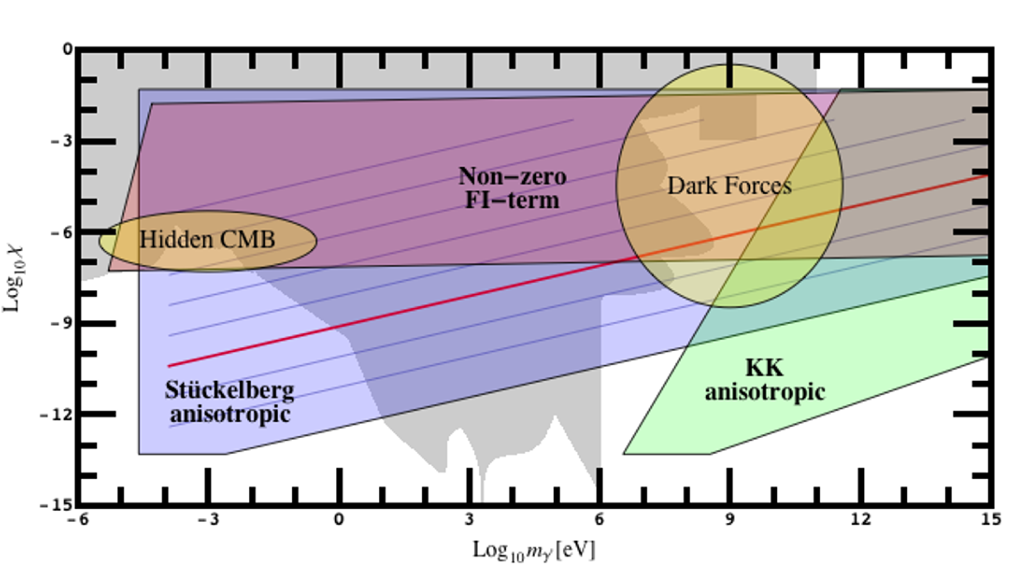
The masses and mixings reachable in this type of setup are shown in Fig. 3 as the light blue area. For large volumes of the cycle supporting the hidden photon we typically also obtain fairly light KK modes of the hidden photon. Assuming that their mixing with the zero mode of the electromagnetic field is of similar size we expect values in the light green area of Fig. 3.

Let us show some interesting values:

•
$\chi\sim 10^{-6}$ gives $m_{\gamma^{\prime}}\sim\kappa\,10^{6}$ GeV and we obtain:
1. 1.
  
  Dark forces: $m_{\gamma^{\prime}}\sim 1$ GeV for $\kappa\sim 10^{-6}$ ,
2. 2.
  
  Hidden CMB: $m_{\gamma^{\prime}}\sim 1$ meV for $\kappa\sim 10^{-18}$ ,
•
$\chi\sim 10^{-7}$ gives $m_{\gamma^{\prime}}\sim\kappa\,10^{3}$ GeV and we obtain:
1. 1.
  
  Dark forces: $m_{\gamma^{\prime}}\sim 1$ GeV for $\kappa\sim 10^{-3}$ ,
2. 2.
  
  Hidden CMB: $m_{\gamma^{\prime}}\sim 1$ meV for $\kappa\sim 10^{-15}$ ,

Therefore we realise that we can reach the dark force regime naturally while we need some amount of fine-tuning to allow for the presence of a hidden CMB.

Let us now check the actual amount of fine tuning and the corresponding value of the overall volume which sets all the fundamental scales in our theory. To do that let us recall that naturally we have $g_{s}\sim 0.1$ . Moreover, $C_{1}^{KK}$ and $C_{12}^{W}$ are unknown functions of the complex structure moduli that can, in principle, be tuned by an appropriate choice of fluxes, however the natural expectation is $C_{1}^{KK}\sim C_{12}^{W}\sim\mathcal{O}(1)$ . Deviations from these natural values require a certain amount of fine-tuning.

Natural Dark Forces for intermediate scale strings

•

$\kappa=2.5\cdot 10^{-6}\sim 10^{-6}$ can be obtained choosing $g_{s}=0.1$ , $C_{1}^{KK}=0.05$ and $C_{12}^{W}=0.1$ corresponding to a kinetic mixing parameter of the order $\chi\sim 10^{-6}$ . The VEVs of the two moduli become $\tau_{1}\sim 10^{-4}\chi^{-2}\sim 10^{8}$ and $\tau_{2}=\tau_{1}/\kappa\sim 10^{14}\gg\tau_{1}$ leading to a volume of the order ${\cal V}\simeq\alpha\sqrt{\tau_{1}}\tau_{2}\sim 10^{17}$ for $\alpha=0.1$ . Thus the string scale turns out to be intermediate $M_{s}\sim 10^{11}$ GeV.
•

$\kappa=10^{-3}$ can be obtained choosing $g_{s}=C_{1}^{KK}=C_{12}^{W}=0.1$ corresponding to a kinetic mixing parameter of the order $\chi\sim 10^{-7}$ . The VEVs of the two moduli become $\tau_{1}\sim 10^{-4}\chi^{-2}\sim 10^{10}$ and $\tau_{2}=\tau_{1}/\kappa\sim 10^{13}\gg\tau_{1}$ leading again to a volume of the order ${\cal V}\simeq\alpha\sqrt{\tau_{1}}\tau_{2}\sim 10^{17}$ for $\alpha=0.1$ together with an intermediate string scale.

We therefore conclude that we can obtain dark forces for natural values of the underlying parameters in scenarios where the string scale is intermediate. These scenarios are favoured also by the fact that TeV-scale supersymmetry can be achieved since the soft masses scale as $M_{soft}\sim W_{0}M_{P}/{\cal V}\sim 1$ TeV for $W_{0}\sim 40$ . Moreover $M_{s}\sim 10^{11}$ GeV yields also a decay constant for the QCD axion in the allowed region and the right Majorana mass scale for right handed neutrinos.

We finally notice that the dark force case corresponds to Calabi-Yau geometries with a slight anisotropy since there is only a mild hierarchy between the characteristic size of the base $L\sim t_{1}^{1/2}=\sqrt{{\cal V}/\tau_{1}}\sim 10^{4}$ and that of the K3 fibre $l\sim\tau_{1}^{1/4}\sim 10^{2}$ .

Hidden CMB with KK Dark Forces and strings at the LHC

•

$\kappa=10^{-15}$ can be obtained choosing $g_{s}=0.01$ , $C_{1}^{KK}\sim 10^{-4}$ and $C_{12}^{W}\sim 10^{3}$ corresponding to a kinetic mixing parameter of the order $\chi\sim 10^{-7}$ . The VEVs of the two moduli become $\tau_{1}\sim 10^{-4}\chi^{-2}\sim 10^{10}$ and $\tau_{2}=\tau_{1}/\kappa\sim 10^{25}\gg\tau_{1}$ leading to a volume of the order ${\cal V}\simeq\alpha\sqrt{\tau_{1}}\tau_{2}\sim 10^{30}$ for $\alpha=1$ . Thus we are in the extreme case of TeV-scale strings: $M_{s}\sim 1$ TeV.
•

$\kappa=10^{-18}$ can be obtained choosing $g_{s}=10^{-3}$ , $C_{1}^{KK}=10^{-4}$ and $C_{12}^{W}=10^{4}$ corresponding to a kinetic mixing parameter of the order $\chi\sim 10^{-6}$ . The VEVs of the two moduli become $\tau_{1}\sim 10^{-4}\chi^{-2}\sim 10^{8}$ and $\tau_{2}=\tau_{1}/\kappa\sim 10^{26}\gg\tau_{1}$ leading again to a volume of the order ${\cal V}\simeq\alpha\sqrt{\tau_{1}}\tau_{2}\sim 10^{30}$ for $\alpha=1$ together with TeV-scale strings.

We therefore conclude that we can obtain a hidden CMB candidate by fine-tuning the values of the underlying parameters in scenarios with $M_{s}\sim 1$ TeV. These scenarios are very promising from several other points of view: they provide a solution to the hierarchy problem that does not rely on supersymmetry, and they might shed new light on the solution of the cosmological constant problem [45].

Furthermore they can be detected in the lab by four different means: via string resonances and deviations from Standard Model quark scattering at the LHC; at light shining through a wall experiments such as ALPS; they lead to large extra dimensions and light moduli mediating long range fifth forces that would give rise to modifications of Newton’s law at the edge of detectability; and the Kaluza-Klein excitations of the hidden gauge bosons are in the Dark Forces regime and could thus be produced in the next generation of experiments searching for these.

We finally notice that the hidden CMB case corresponds to Calabi-Yau three-fold with a very anisotropic shape since there is a large hierarchy between the characteristic size of the base $L\sim t_{1}^{1/2}=\sqrt{{\cal V}/\tau_{1}}\sim 10^{11}$ and that of the K3 fibre $l\sim\tau_{1}^{1/4}\sim 10^{2}$ .

5.2 Non-zero FI-term

Fixing $\tau_{1}$ via the interplay of $D$ -terms and string loop corrections to the Kähler potential we can rewrite the relation (54) between $m_{\gamma^{\prime}}$ and $\chi$ as:

m_{\gamma^{\prime}}\simeq 10^{20}\alpha f_{2}\frac{\sqrt{\tau_{1}}}{{\cal V}}\chi\text{\ GeV}\simeq 5\cdot 10^{17}\alpha\frac{f_{2}}{{\cal V}}\text{\ GeV}.

(119)

Substituting in (119) the expression (93) for the VEV of $\tau_{1}$ in terms of $\chi$ , we end up with:

m_{\gamma^{\prime}}\simeq 5\cdot 10^{17}\mu_{1}\,e^{-\mu_{2}\chi^{-2}}\text{\ GeV},

(120)

where $\mu_{1}=\alpha f_{2}$ and $\mu_{2}=25\cdot 10^{-6}\sigma^{-1}$ , with $\sigma$ that is a free parameter whose value is fixed by the requirement of getting a Minkowski vacuum:

\langle\tau_{1}\rangle=\sigma\ln\langle{\cal V}\rangle,\text{ \ \ \ \ with \ \ \ \ }\sigma\equiv\frac{324\pi^{2}c_{1}^{2}}{a_{3}^{3}f_{2}^{2}}.

(121)

Varying the integers in this equation within reasonable limits ( $1-10$ ) we can reach values within the red area of Fig. 3.

Let us now illustrate the phenomenological implications of these results with the help of some parameter fits that lead to $\chi\simeq 10^{-6}$ . The dark force case with $m_{\gamma^{\prime}}\sim 1$ GeV can be achieved for $\mu_{1}=0.1$ and $\mu_{2}=4.1565\cdot 10^{-11}$ . These two values can be obtained choosing $\alpha=0.1$ , $f_{2}=1$ , $c_{1}=8$ and $a_{3}=2\pi/N_{3}$ with $N_{3}=9$ . The VEV of the K3 divisor becomes $\tau_{1}\simeq 25\cdot 10^{-6}\chi^{-2}=2.5\cdot 10^{7}$ while the volume is of the order ${\cal V}\simeq e^{\tau_{1}/\sigma}\sim 10^{18}$ corresponding to an intermediate string scale. Given that the volume can be also expressed as $a_{3}\ln{\cal V}\simeq\xi^{2/3}/g_{s}$ , we can choose $\xi=1.5$ and $g_{s}=0.045$ . Using (92), we can finally check that no fine-tuning of the string loop corrections is needed in order to get a vanishing cosmological constant since the above choice of parameters sets $C_{1}^{KK}\simeq 1.63$ .

We therefore conclude that, even in this case where the K3 divisor is fixed by the interplay of $D$ -terms and $g_{s}$ corrections, we can obtain dark forces for natural values of the underlying parameters in scenarios where the string scale is intermediate. However this case looks less promising than the one with vanishing FI-terms since the additional constaint coming from the requirement of a viable up-lifting reduces the reliability of our predictions. In fact, due to the exponential dependence of $m_{\gamma^{\prime}}$ on $\chi$ , a small change in our choice of parameters gives drastic changes for the mass of the hidden photon at fixed kinetic mixing. For example, if we just change $c_{1}=8$ to $c_{1}=7$ in the above fit, the prediction for the $U(1)$ mass gets modified from $m_{\gamma^{\prime}}\simeq 1$ GeV to $m_{\gamma^{\prime}}\simeq 10^{-6}$ GeV.

With other small changes, like $\alpha=0.1\to 10$ and $c_{1}=8\to 6$ , we can easily reach the interesting hidden CMB regime for $m_{\gamma^{\prime}}\sim 1$ meV. The VEV of the K3 divisor is still of the order $\tau_{1}\simeq 10^{7}$ while the volume now becomes ${\cal V}\simeq e^{\tau_{1}/\sigma}\sim 10^{32}$ corresponding to the extreme case of TeV-scale strings. Such a large value of ${\cal V}$ can be obtained for $\xi=1.5$ and $g_{s}=0.025$ . Using (92), we can finally check that, contrary to the dark force case, the upliting now requires a large fine-tuning of the coefficient of the loop corrections of the order $C_{1}^{KK}\simeq 3.3\cdot 10^{-7}$ .

6 Conclusions

We have shown that allowing for anisotropy in LARGE volume compactifications greatly enhances the phenomenological possibilities for hidden D-brane $U(1)$ s. In this case, in addition to collapsed, small, or hyperweak cycles, it is possible to wrap (hidden) branes on “milliweak” cycles. Each of these will give different ranges of gauge couplings and thus kinetic mixing with the hypercharge, but since in this case the Stückelberg masses of the $U(1)$ s become more weakly correlated with the volume of the cycle, a milliweak cycle allows for the attractive possibility of a very small mass but moderate (and thus observable) mixing.

In fact, naively there is an embarrassment of riches; the possible masses and mixings become so diverse as to render the scenario almost unpredictive, with the exception of lower bounds due to there being a maximum volume of the compactification (of $\mathcal{V}\sim 10^{30}$ since the string scale cannot be below $\mathcal{O}(\mathrm{TeV})$ ). We therefore considered the constraints imposed by insisting on moduli stabilisation, taking careful account of the relationship between fluxes required to give the $U(1)$ s masses and the presence of D-terms and hidden chiral matter. These constraints then translate into requirements on uncalculable parameters in the model such as the coefficients of the loop corrections to the Kähler potential. We found that without any fine-tuning it is possible to have hidden $U(1)$ s in the Dark Forces regime even for intermediate scale strings, and so we could soon be probing intermediate scale string effects in the lab!

We also found that we can realise the “hidden CMB” scenario of a hidden $U(1)$ of mass $\sim$ meV and mixing $\sim 10^{-6}$ , with the price being some fine tuning. In compensation we surprisingly find multiple ways to test it: other than cosmological observations, it can be directly tested in lab experiments at very low energies, in Dark Forces experiments due to the hidden Kaluza-Klein modes, and at the LHC since the string scale must be low.

We hope that we have provided ample motivation and tools to search for these setups in more complete models, including explicit brane constructions with tadpole cancellation. The reward for this endeavour would be a way to probe in the lab the hidden sectors that generically arise, and interesting hidden sector model building.

7 Acknowledgements

We would like to thank Fernando Quevedo for useful discussions, and the organisers of the XXIII Bad Honnef “Beyond the Standard Model” workshop for hospitality while this paper was in the final stages of preparation. MDG is supported by the German Science Foundation (DFG) under SFB 676.

Appendix A $U(1)$ masses from dimensional reduction

A.1 U(1) factors from D-branes

A very important ingredient of Calabi-Yau flux compactifications is the presence of $Dp$ -branes which wrap internal $(p-3)$ -cycles and have to fill the four-dimensional space-time in order not to break Poincaré invariance. Each space-time filling $Dp$ -brane comes along with a $U(1)$ gauge theory that lives on its world volume. Thus string compactifications naturally come along with many $U(1)$ gauge bosons.

The dynamics of a $Dp$ -brane is governed by the Dirac-Born-Infeld action $S_{DBI}$ together with a Chern-Simons action $S_{CS}$ :

	$\displaystyle S_{DBI}$	$\displaystyle=$	$\displaystyle-\mu_{p}e^{-\phi}\int_{\mathcal{W}}d^{p+1}\xi\sqrt{-\textrm{det}\left[\imath^{*}(G+B_{2})+l_{s}^{2}F_{2}/(2\pi)\right]},$		(122)
	$\displaystyle S_{CS}$	$\displaystyle=$	$\displaystyle\mu_{p}e^{-\phi}\int_{\mathcal{W}}\sum_{p}\imath^{}\left(C_{p}\right)\wedge e^{\imath^{}(B_{2})+l_{s}^{2}F_{2}/(2\pi)},$		(123)

where $\phi$ is the dilaton, $\mu_{p}$ is the tension of the $Dp$ -brane which is equal to its RR-charge since the $Dp$ -brane has to satisfy a BPS condition, $G$ denotes the 10D metric, $B_{2}$ is the NS-NS 2-form, $F_{2}$ is the gauge field strength, and $C_{p}$ is a R-R $p$ -form. The integrals in (122) and (123) are taken over the $(p+1)$ -dimensional world-volume $\mathcal{W}$ of the $Dp$ -brane, which is embedded in the ten dimensional space-time manifold $\mathcal{X}_{10}=\mathbb{R}^{3,1}\times\mathcal{M}_{6}$ , where $\mathcal{M}_{6}$ is a 6D Calabi-Yau manifold, via the map $\imath:\mathcal{W}\hookrightarrow\mathcal{X}_{10}$ . $\imath^{*}$ denotes the pullback operation.

From now on, we shall focus on type IIB flux compactifications since this is the context where moduli stabilisation is best understood. We shall also be interested in the case of a $D7$ -brane wrapping an internal 4-cycle $D$ which is a smooth divisor of the Calabi-Yau three-fold. The volume of a generic 4-cycle $D_{i}$ is given by the real part of the Kähler modulus $T_{i}$ which in 4D Einstein-frame is defined as:

T_{i}\equiv\left(\int_{D_{i}}\sqrt{g}\,d^{4}y+i\int_{D_{i}}C_{4}\right)\frac{e^{-\phi}}{l_{s}^{4}}\equiv\tau_{i}+ib_{i},\,\,\,\,\,\,\,\,\,i=1,...,h_{1,1},

(124)

where $h_{1,1}$ is one of the Calabi-Yau Hodge numbers and $C_{4}$ is the 10D R-R 4-form.

The standard Maxwell action can be obtained from expanding the DBI action (122) in powers of the field strength⁹⁹ 9 We are neglecting the background NSNS two-form $B_{2}$ since we shall look at orientifold projections such that $h_{1,1}^{-}=0$ .:

	$\displaystyle S_{DBI}$	$\displaystyle=$	$\displaystyle-\mu_{7}e^{-\phi}\int_{\mathbb{R}^{3,1}\times D_{i}}d^{8}\xi\sqrt{-\textrm{det}\left[\varphi^{*}(G)+l_{s}^{2}F_{2}/(2\pi)\right]}$		(125)
		$\displaystyle=$	$\displaystyle-\mu_{7}e^{-\phi}\int_{\mathbb{R}^{3,1}\times D_{i}}d^{8}\xi\sqrt{-\textrm{det}\left[\varphi^{*}(G)\right]}\left(1+\frac{l_{s}^{4}}{16\pi^{2}}F_{MN}F^{MN}-\frac{l_{s}^{8}}{128\pi^{4}}\left(F_{MN}F^{MN}\right)^{2}+...\right),$		(125)

and then performing the dimensional reduction from 8D to 4D:

-\frac{\mu_{7}e^{-\phi}l_{s}^{4}}{16\pi^{2}}\int_{\mathbb{R}^{3,1}\times D_{i}}d^{8}\xi\sqrt{-\textrm{det}\left[\varphi^{*}(G)\right]}F_{MN}F^{MN}\,\,\,\,\rightarrow\,\,\,\,-\left(\frac{\mu_{7}l_{s}^{8}}{16\pi^{2}}\right)\tau_{i}\int_{\mathbb{R}^{3,1}}F_{\mu\nu}F^{\mu\nu}d^{4}x.

The $D7$ -brane tension is given by $\mu_{7}=2\pi/(g_{s}l_{s}^{8})$ , and so we obtain the final result:

\mathcal{L}_{kin}=-\frac{1}{4g_{i}^{2}}\int_{\mathbb{R}^{3,1}}F_{\mu\nu}F^{\mu\nu}d^{4}x\,\,\,\,\,\,\text{with}\,\,\,\,\,\,g_{i}^{2}=\frac{2\pi}{\tau_{i}}.

(126)

A.2 Massive U(1)s from internal fluxes

A $U(1)$ gauge boson living on a $D7$ -brane can acquire a mass by turning on an internal magnetic flux in the world-volume of the $D7$ -brane. In fact, turning on a 2-form gauge flux on a 2-cycle internal to the 4-cycle wrapped by the $D7$ generates a coupling between the $U(1)$ gauge boson and the Kähler modulus (124) corresponding to the 4-cycle Poincaré dual to the 2-cycle supporting the magnetic flux. Then the axion, that is the imaginary part of the charged Kähler modulus, gets eaten up by the $U(1)$ gauge boson which becomes massive via the Stückelberg mechanism. This is the way in which string theory cures any problem coming from dangerous anomalous $U(1)$ s which acquire $\mathcal{O}(M_{s})$ -masses through the Green-Schwarz mechanism, and so they disappear from the 4D effective field theory. However we shall be interested in non-anomalous $U(1)$ s which can still become massive via the same mechanism, but their mass can be much lighter than $M_{s}$ . Therefore these hidden photons have to be included in the description of the 4D effective field theory coming from string compactifications.

Let us see more in detail how this happens. The expansion of the Chern-Simons action (123) contains a coupling with the 10D R-R 4-form $C_{4}$ which looks like:

\mathcal{L}\supset-2\pi\frac{e^{-\phi}}{l_{s}^{2}}\int_{\mathbb{R}^{3,1}\times D_{i}}\frac{F_{2}}{2\pi}\wedge C_{4}\wedge\frac{F_{2}}{2\pi}.

(127)

The R-R form $C_{4}$ can be decomposed as:

C_{4}=Q_{2}^{i}(x)\wedge\hat{D}_{i}(y)+b_{i}(x)\tilde{D}^{i}(y),\text{ \ \ }i=1,...,h_{1,1},

(128)

where the $\tilde{D}_{i}$ are a basis of harmonic (2,2)-forms of $H_{2,2}(\mathcal{M}_{6})$ , dual to the (1,1)-forms $\hat{D}_{i}$ , while the 4D fields $b_{i}(x)$ are the axions defined in (124) and $Q_{2}^{i}(x)$ are 2-forms dual to the $b_{i}(x)$ (due to the self-duality of $F_{5}=dC_{4}=\star_{10D}F_{5}$ ). Taking both of the $F$ ’s to be with non-compact indices, and reducing $C_{4}$ along the divisor $D_{i}$ , gives rise to the axion-dependent CP-odd coupling:

\mathcal{L}\supset-\frac{e^{-\phi}}{2\pi l_{s}^{4}}\left(\int_{D_{i}}C_{4}\right)\int_{\mathbb{R}^{3,1}}F_{2}\wedge F_{2}=\frac{b_{i}}{2\pi}\int_{\mathbb{R}^{3,1}}F_{2}\wedge F_{2},

(129)

which combined with the result (126) for the CP-even coupling, yields the following expression for the gauge kinetic function:

f_{D7_{i}}=\frac{T_{i}}{2\pi}.

(130)

On the other hand, taking one of the $F$ ’s to be the compact flux (denoted as $F^{c}_{2}$ ) and the other to be with non-compact indices, we obtain (working in Einstein frame):

\mathcal{L}\supset-\frac{1}{2\pi l_{s}^{4}}\left(\int_{D_{i}}\hat{D}_{j}\wedge F^{c}_{2}\right)\int_{\mathbb{R}^{3,1}}Q_{2}^{j}\wedge F_{2}=\frac{q_{ij}}{l_{s}^{2}}\int_{\mathbb{R}^{3,1}}Q_{2}^{j}\wedge F_{2},

(131)

where $q_{ij}$ is the charge of the 2-form $Q_{2}^{j}$ under the $U(1)$ living on the divisor $D_{i}$ . Expanding the gauge flux $F^{c}_{2}$ in the basis of (1,1)-forms $\hat{D}_{i}$ as $F^{c}_{2}=f_{c}^{i}\hat{D}_{i}$ , and defining the Calabi-Yau intersection numbers as:

k_{ijk}=\frac{1}{l_{s}^{6}}\int_{\mathcal{M}_{6}}\hat{D}_{i}\wedge\hat{D}_{j}\wedge\hat{D}_{k},

(132)

we end up with the following expression for the $U(1)$ -charge $q_{ij}$ :

q_{ij}=\frac{1}{2\pi l_{s}^{2}}\int_{D_{i}}\hat{D}_{j}\wedge F^{c}_{2}=\frac{f_{c}^{k}}{2\pi l_{s}^{6}}\int_{\mathcal{M}_{6}}\hat{D}_{i}\wedge\hat{D}_{j}\wedge\hat{D}_{k}=\frac{f_{c}^{k}}{2\pi}k_{ijk}.

(133)

Therefore the gauge flux coefficients and the intersection numbers determine which 2-forms couple to the Abelian gauge boson which lives on the divisor $D_{i}$ . Recalling that the 2-forms $Q_{2}^{j}(x)$ are 4D dual to the axions $b_{j}(x)$ , we realise that the Kähler moduli which get charged under the $U(1)$ , are those parameterising the volume of 4-cycles that intersect the 2-cycle supporting the gauge flux. This is topologically equivalent to saying that the Kähler moduli which get a $U(1)$ -charge are a combination of 4-cycles corresponding to the 4-cycle that is Poincaré dual to the 2-cycle on which the magnetic flux is turned on. Due to the coupling (131), the $U(1)$ gauge boson becomes massive by eating the axion (or an appropriate combination of axions) which is the imaginary part of the charged Kähler modulus.

In order to see this mechanism in more detail, we need to include also the kinetic terms for the $Q_{2}^{j}$ which are expressed in terms of the corresponding field strength $H_{3}^{j}=dQ_{2}^{j}$ . They can be derived from the 10D term $S\supset-\frac{1}{8\kappa_{10}^{2}}\int F_{5}\wedge\star F_{5}$ :

-\frac{2\pi}{4l_{s}^{6}}\int_{\mathbb{R}^{3,1}\times\mathcal{M}_{6}}dC_{4}\wedge*dC_{4}=-\frac{\pi}{l_{s}^{2}}\left(\int_{\mathcal{M}_{6}}\hat{D}_{j}\wedge*\hat{D}_{k}\right)\int_{\mathbb{R}^{3,1}}\frac{1}{2}dQ_{2}^{j}\wedge*dQ_{2}^{k},

(134)

where:

\frac{1}{l_{s}^{6}}\int_{\mathcal{M}_{6}}\hat{D}_{j}\wedge*\hat{D}_{k}=\frac{(\mathcal{K}_{0}^{-1})_{jk}}{{\cal V}},

(135)

with ${\cal V}$ the dimensionless Calabi-Yau volume. The matrix $\mathcal{K}^{-1}_{0}$ is defined as the inverse of the metric obtained by taking the second derivatives of the tree-level Kähler potential $K_{0}=-2\ln{\cal V}$ with respect to the real part of the $T$ -moduli. Thus we end up with:

-\pi\frac{(\mathcal{K}^{-1}_{0})_{jk}}{{\cal V}l_{s}^{2}}\int_{\mathbb{R}^{3,1}}\frac{1}{2}dQ_{2}^{j}\wedge*dQ_{2}^{k}=-\pi\frac{(\mathcal{K}^{-1}_{0})_{jk}}{{\cal V}l_{s}^{2}}\int_{\mathbb{R}^{3,1}}\frac{1}{12}H_{\mu\nu\rho}^{j}H^{k,\mu\nu\rho}d^{4}x.

(136)

Our final Lagrangian is then given by the standard Maxwell action (126) plus the term (131) describing the coupling of the 2-form $Q_{2}^{j}$ to the Abelian gauge boson and the 2-form kinetic term (136). Before showing how the gauge boson becomes massive, let us redefine the 2-form so that it gets a canonical mass dimension 1:

Z_{2}^{j}\equiv M_{P}Q_{2}^{j}\,\,\,\,\,\,\,\,\Leftrightarrow\,\,\,\,\,\,\,\,G_{3}^{j}\equiv M_{P}H_{3}^{j}.

(137)

Using $l_{s}^{-2}=M_{s}^{2}=M_{P}^{2}/(4\pi{\cal V})$ , the final Lagrangian takes the form:

\mathcal{L}=-\frac{(\mathcal{K}^{-1}_{0})_{jk}}{48{\cal V}^{2}}G_{\mu\nu\rho}^{j}G^{k,\mu\nu\rho}-\frac{1}{4g_{i}^{2}}F_{\mu\nu}F^{\mu\nu}+q_{ij}\frac{M_{P}}{4\pi{\cal V}}Z_{2}^{j}\wedge F_{2}.

(138)

The 2-form kinetic terms can be canonically normalised by defining (suppressing the space-time indices):

G^{i}=2{\cal V}\,C^{i}_{j}\mathcal{H}^{j},\,\,\,\,\Leftrightarrow\,\,\,\,Z_{2}^{i}=2{\cal V}\,C^{i}_{j}\mathcal{D}_{2}^{j},

(139)

where the columns of the matrix $C^{i}_{j}$ are given by the eigenvectors of $K^{-1}_{0}$ normalised as:

(\mathcal{K}_{0}^{-1})_{ij}C^{j}_{a}=C_{ia}\lambda_{a},\text{ \ \ \ with \ \ \ }(C^{t})_{a}^{i}C_{ib}=\lambda_{a}^{-1}\delta_{ab}.

(140)

Note that

(C^{t})_{b}^{i}(\mathcal{K}_{0}^{-1})_{ij}C^{j}_{a}=\delta_{ab}\rightarrow(C^{t})_{b}^{i}(\mathcal{K}_{0}^{-1})_{ij}C^{j}_{a}(C^{t})^{a}_{k}=(C^{t})^{b}_{k}\rightarrow C^{j}_{a}(C^{t})^{a}_{k}=(\mathcal{K}_{0})_{ik}.

(141)

Canonically normalising also the $U(1)$ field strength as $F=g_{i}\mathcal{F}^{i}$ , and using the expressions (126) and (7) for the coupling constant $g_{i}$ and the $U(1)$ -charge $q_{ij}$ respectively, we end up with (defining the dimensionless flux coefficients $f^{i}$ as $f^{i}\equiv l_{s}^{2}f_{c}^{i}/(2\pi)$ ):

\mathcal{L}=-\frac{1}{12}\mathcal{H}_{\mu\nu\rho}^{j}\mathcal{H}_{j}^{\mu\nu\rho}-\frac{1}{4}\mathcal{F}_{\mu\nu}^{i}\mathcal{F}^{i\,\mu\nu}+M_{ij}\mathcal{D}_{2}^{j}\wedge\mathcal{F}_{2}^{i}.

(142)

where:

M_{ij}\equiv\left(g_{i}f^{k}k_{ipk}C^{p}_{j}\right)\frac{M_{P}}{2\pi}=\left(g_{i}\,q_{ip}C^{p}_{j}\right)\frac{M_{P}}{2\pi}.

(143)

with no sum over $i$ since this index simply denotes the 4-cycle $D_{i}$ wrapped by the $D7$ -brane. Hence we realise that in general $F_{2}$ couples to a particular combination of all the 2-forms, and not just to a single 2-form, due to the canonical normalisation which typically introduces a mixing among all the 2-forms.

Let us see why on dualising $\mathcal{D}_{2}$ to the corresponding axion $a$ , the Lagrangian (142) generates an explicit mass term $m_{\gamma^{\prime}}^{2}\mathcal{A}_{\mu}\mathcal{A}^{\mu}$ for the $U(1)$ gauge boson. The dual axion $a$ can be introduced as a Lagrange multiplier for the arbitrary field $\mathcal{H}_{\mu\nu\rho}$ by imposing the constraint $d^{*}\mathcal{H}=0$ which is locally equivalent to $d\mathcal{D}_{2}=\mathcal{H}$ :

\mathcal{L}=-\frac{1}{12}\mathcal{H}_{\mu\nu\rho}^{j}\mathcal{H}_{j}^{\mu\nu\rho}-\frac{1}{4}\mathcal{F}_{\mu\nu}\mathcal{F}^{\mu\nu}-\frac{M_{ij}}{6}\ \epsilon^{\mu\nu\rho\sigma}\mathcal{H}^{j}_{\mu\nu\rho}\ A_{\sigma}-\frac{M_{ij}}{6}\,a\epsilon^{\mu\nu\rho\sigma}\partial_{\mu}\mathcal{H}^{j}_{\nu\rho\sigma}.

(144)

We can now obtain a quadratic Lagrangian for $\mathcal{H}$ by integrating by parts the last term in (144). Then the equations of motion for $\mathcal{H}$ give:

\mathcal{H}_{j}^{\mu\nu\rho}=-{M_{ij}}\ \epsilon^{\mu\nu\rho\sigma}\left(A_{\sigma}+\partial_{\sigma}a\right),

(145)

which inserted back into (144) yields:

\mathcal{L}=-\frac{1}{4}\mathcal{F}_{\mu\nu}\mathcal{F}^{\mu\nu}-\frac{m_{\gamma^{\prime}}^{2}}{2}\left(A_{\mu}+\partial_{\mu}a\right)\left(A^{\mu}+\partial^{\mu}a\right),\text{ \ \ \ with \ \ \ }m_{\gamma^{\prime}}^{2}=\sum_{j}M_{ij}^{2}.

(146)

The field $\mathcal{A}_{\mu}\equiv A_{\mu}+\partial_{\mu}a$ clearly represents a massive $U(1)$ gauge boson. Thus the axion $a$ is eaten up by the gauge boson without the need of any Higgs-like field in a stringy realisation of the standard Stückelberg mechanism. Note that the above can be simplified using 141 to

	$\displaystyle(M^{2})_{ab}=$	$\displaystyle M_{aj}M^{t}_{jb}=\frac{M_{P}^{2}}{2\pi\sqrt{\tau_{a}\tau_{b}}}q_{ap}C^{p}_{j}(C^{t})^{j}_{r}q_{br}$
	$\displaystyle=$	$\displaystyle\frac{M_{P}^{2}}{2\pi\sqrt{\tau_{a}\tau_{b}}}q_{ap}q_{br}(\mathcal{K}_{0})_{pr}.$		(147)

If we include also the contributions from four-cycles odd under the orientifold $\hat{D}^{c}_{-}$ , defining

\displaystyle r_{ac}\equiv\int_{D_{a}}\hat{D}^{c}_{-},

(148)

the final total result is

\displaystyle m_{ab}^{2}=

\displaystyle g_{a}g_{b}\,\frac{M_{P}^{2}}{4\pi^{2}}\bigg[\mathcal{V}^{-2}r_{ac}(\mathcal{K}_{0}^{-1})^{cd}r_{bd}+q_{a\alpha}(\mathcal{K}_{0})_{\alpha\beta}q_{b\beta}\bigg].

(149)

This expression is equivalent to the one presented in [10] noting the different metrics used and the different definition of $M_{s}$ .

A.3 FI-terms

In the previous section we have seen how $U(1)$ gauge bosons can acquire a mass by turning on an internal magnetic flux in the world-volume of a $D7$ -brane wrapping a divisor $D_{i}$ with corresponding Kähler modulus $T_{i}$ . This guarantees that also a moduli-dependent 4D Fayet-Iliopoulos term gets generated [71, 72, 73]. In fact, denoting as $T_{U(1)}$ the charged Kähler modulus which is in general a combination of all the basis divisors corresponding to the 4-cycle Poincaré dual to the 2-cycle supporting the magnetic flux, the axion $a=\text{Im}(T_{U(1)})$ gets eaten up by the $U(1)$ gauge boson via the Stückelberg mechanism, but $\tau=\text{Re}(T_{U(1)})$ is a light modulus that has to be taken into account in the effective field theory and gives rise to a moduli-dependent Fayet-Iliopoulos term.

This can be seen to arise from the low-energy reduction of the DBI action (125):

S_{DBI}=-\mu_{7}e^{-\phi}\Gamma(y)\int_{\mathbb{R}^{3,1}}d^{4}x\left(1+\frac{l_{s}^{4}}{16\pi^{2}}F_{\mu\nu}(x)F^{\mu\nu}(x)+...\right),

(150)

where:

\Gamma(y)=\int_{D_{i}}d^{4}y\sqrt{-\textrm{det}\left[\varphi^{*}(g_{CY})\right]}\left(1+\frac{l_{s}^{4}}{16\pi^{2}}F_{mn}(y)F^{mn}(y)+...\right).

From the BPS calibration condition for a $D7$ -brane we find that:

\Gamma(y)=\frac{1}{2}\int_{D_{i}}\left(J\wedge J-\frac{l_{s}^{4}}{4\pi^{2}}F_{2}^{c}\wedge F_{2}^{c}\right)+\frac{\left(\int_{D_{i}}J\wedge\frac{l_{s}^{2}}{2\pi}F_{2}^{c}\right)^{2}}{\int_{D_{i}}\left(J\wedge J-\frac{l_{s}^{4}}{4\pi^{2}}F_{2}^{c}\wedge F_{2}^{c}\right)}.

(151)

When in (150) $\Gamma(y)$ multiplies the first term in parenthesis, after performing the appropriate Weyl rescaling to 4D Einstein frame¹⁰¹⁰ 10 We recall that the 10D metric in string frame is related to the 10D metric in Einstein frame via $g_{MN}^{(s)}=e^{\phi/2}g_{MN}^{(E)}$ ., we obtain two contributions to the 4D scalar potential: the $D7$ -brane tension $T_{D7}$ and a moduli dependent Fayet-Iliopoulos term $\xi_{i}$ :

T_{D7}=g_{i}^{-2}4\pi^{2}e^{2\phi}M_{s}^{4},\text{ \ \ and \ \ }V_{D}=\frac{g_{i}^{2}}{2}\xi_{i}^{2},\text{ \ \ with \ \ }\frac{\xi_{i}}{M_{P}^{2}}=\frac{1}{4\pi{\cal V}}\int_{D_{i}}\left(J\wedge\frac{l_{s}^{2}}{2\pi}F^{c}_{2}\right).

(152)

The $D7$ -brane tension gives no net contribution to the scalar potential since it will be compensated by by other extended objects due to tadpole cancellation.

On the other hand, considering in (150) $\Gamma(y)$ multiplied by the second term in parenthesis, we realise that in the presence of a non-vanishing world-volume flux, the expression (126) for the gauge coupling constant $g_{i}$ gets modified to:

\frac{2\pi}{g_{i}^{2}}=\text{Re}(T_{i})-h_{i}(F_{2}^{c})\text{Re}(S),

(153)

where $\text{Re}(S)=e^{-\phi}$ and the flux-dependent factor is given by $h_{i}(F_{2}^{c})=\frac{f^{k}f^{j}k_{ijk}}{2}=\frac{f^{j}q_{ij}}{2}$ where $q_{ij}$ are the flux-dependent $U(1)$ charges of the Kähler moduli (7).

The Fayet-Iliopoulos term in (152) can be rewritten as:

\frac{\xi_{i}}{M_{P}^{2}}=\frac{1}{4\pi{\cal V}}\int_{D_{i}}\left(J\wedge\frac{l_{s}^{2}}{2\pi}F^{c}_{2}\right)=\frac{1}{4\pi{\cal V}}t^{j}f^{k}k_{ijk}=\frac{q_{ij}}{4\pi}\frac{t^{j}}{{\cal V}}=-\frac{q_{ij}}{4\pi}\frac{\partial K}{\partial\tau_{j}}.

(154)

V_{D}=\frac{g_{i}^{2}}{2}\left(\sum_{j}c_{ij}\varphi_{j}\frac{\partial K}{\partial\varphi_{j}}-\xi_{i}\right)^{2}=\frac{\pi}{\left(\tau_{i}-f^{j}q_{ij}/(2g_{s})\right)}\left(\sum_{j}c_{ij}\varphi_{j}\frac{\partial K}{\partial\varphi_{j}}+\frac{q_{ij}}{4\pi}\frac{\partial K}{\partial\tau_{j}}\right)^{2}.

(155)

References

[1] L. B. Okun, Limits of electrodynamics: Paraphotons?, Sov. Phys. JETP 56 (1982) 502.
[2] B. Holdom, Two U(1)’s and Epsilon Charge Shifts, Phys. Lett. B166 (1986) 196.
[3] K. R. Dienes, C. F. Kolda and J. March-Russell, Kinetic mixing and the supersymmetric gauge hierarchy, Nucl. Phys. B492 (1997) 104–118 [hep-ph/9610479].
[4] A. Lukas and K. S. Stelle, Heterotic anomaly cancellation in five dimensions, JHEP 01 (2000) 010 [hep-th/9911156].
[5] S. A. Abel and B. W. Schofield, Brane-antibrane kinetic mixing, millicharged particles and SUSY breaking, Nucl. Phys. B685 (2004) 150–170 [hep-th/0311051].
[6] R. Blumenhagen, G. Honecker and T. Weigand, Loop-corrected compactifications of the heterotic string with line bundles, JHEP 06 (2005) 020 [hep-th/0504232].
[7] S. A. Abel, J. Jaeckel, V. V. Khoze and A. Ringwald, Illuminating the hidden sector of string theory by shining light through a magnetic field, Phys. Lett. B666 (2008) 66–70 [hep-ph/0608248].
[8] S. A. Abel, M. D. Goodsell, J. Jaeckel, V. V. Khoze and A. Ringwald, Kinetic Mixing of the Photon with Hidden U(1)s in String Phenomenology, JHEP 07 (2008) 124 [0803.1449].
[9] M. Goodsell, Light Hidden U(1)s from String Theory, 0912.4206.
[10] M. Goodsell, J. Jaeckel, J. Redondo and A. Ringwald, Naturally Light Hidden Photons in LARGE Volume String Compactifications, JHEP 11 (2009) 027 [0909.0515].
[11] M. Goodsell and A. Ringwald, Light hidden-sector U(1)s in string compactifications, Fortsch. Phys. 58 (2010) 716–720 [1002.1840].
[12] J. J. Heckman and C. Vafa, An Exceptional Sector for F-theory GUTs, Phys. Rev. D83 (2011) 026006 [1006.5459].
[13] M. Bullimore, J. P. Conlon and L. T. Witkowski, Kinetic mixing of U(1)s for local string models, JHEP 11 (2010) 142 [1009.2380].
[14] J. Jaeckel, J. Redondo and A. Ringwald, Signatures of a hidden cosmic microwave background, Phys. Rev. Lett. 101 (2008) 131801 [0804.4157].
[15] WMAP Collaboration, E. Komatsu et. al., Seven-Year Wilkinson Microwave Anisotropy Probe (WMAP) Observations: Cosmological Interpretation, Astrophys. J. Suppl. 192 (2011) 18 [1001.4538].
[16] M. Ahlers, H. Gies, J. Jaeckel, J. Redondo and A. Ringwald, Light from the Hidden Sector, Phys. Rev. D76 (2007) 115005 [0706.2836].
[17] M. Ahlers, H. Gies, J. Jaeckel, J. Redondo and A. Ringwald, Laser experiments explore the hidden sector, Phys. Rev. D77 (2008) 095001 [0711.4991].
[18] ALPS Collaboration, K. Ehret et. al., New ALPS Results on Hidden-Sector Lightweights, Phys. Lett. B689 (2010) 149–155 [1004.1313].
[19] M. Fouche et. al., Search for photon oscillations into massive particles, Phys. Rev. D78 (2008) 032013 [0808.2800].
[20] A. Afanasev et. al., New Experimental Limit on Photon Hidden-Sector Paraphoton Mixing, Phys. Lett. B679 (2009) 317–320 [0810.4189].
[21] P. Arias, J. Jaeckel, J. Redondo and A. Ringwald, Optimizing Light-Shining-through-a-Wall Experiments for Axion and other WISP Searches, Phys. Rev. D82 (2010) 115018 [1009.4875].
[22] J. Jaeckel, J. Redondo and A. Ringwald, Hidden Laser Communications Through Matter -An application of meV-scale hidden photons-, Europhys. Lett. 87 (2009) 10010 [0903.5300].
[23] F. Hoogeveen, Terrestrial axion production and detection using RF cavities, Phys. Lett. B288 (1992) 195–200.
[24] J. Jaeckel and A. Ringwald, A Cavity Experiment to Search for Hidden Sector Photons, Phys. Lett. B659 (2008) 509–514 [0707.2063].
[25] F. Caspers, J. Jaeckel and A. Ringwald, Feasibility, engineering aspects and physics reach of microwave cavity experiments searching for hidden photons and axions, JINST 4 (2009) P11013 [0908.0759].
[26] R. G. Povey, J. G. Hartnett and M. E. Tobar, Microwave cavity light shining through a wall optimization and experiment, Phys. Rev. D82 (2010) 052003 [1003.0964].
[27] ADMX Collaboration, A. Wagner et. al., A Search for Hidden Sector Photons with ADMX, Phys. Rev. Lett. 105 (2010) 171801 [1007.3766].
[28] J. Redondo, Helioscope Bounds on Hidden Sector Photons, JCAP 0807 (2008) 008 [0801.1527].
[29] J. Jaeckel and A. Ringwald, The Low-Energy Frontier of Particle Physics, Ann. Rev. Nucl. Part. Sci. 60 (2010) 405–437 [1002.0329].
[30] N. Arkani-Hamed, D. P. Finkbeiner, T. R. Slatyer and N. Weiner, A Theory of Dark Matter, Phys. Rev. D79 (2009) 015014 [0810.0713].
[31] N. Arkani-Hamed and N. Weiner, LHC Signals for a SuperUnified Theory of Dark Matter, JHEP 12 (2008) 104 [0810.0714].
[32] M. Pospelov and A. Ritz, Astrophysical Signatures of Secluded Dark Matter, Phys. Lett. B671 (2009) 391–397 [0810.1502].
[33] D. E. Morrissey, D. Poland and K. M. Zurek, Abelian Hidden Sectors at a GeV, JHEP 07 (2009) 050 [0904.2567].
[34] D. Feldman, Z. Liu, P. Nath and G. Peim, Multicomponent Dark Matter in Supersymmetric Hidden Sector Extensions, Phys. Rev. D81 (2010) 095017 [1004.0649].
[35] Y. Mambrini, The kinetic dark-mixing in the light of CoGENT and XENON100, JCAP 1009 (2010) 022 [1006.3318].
[36] M. Pospelov, Secluded U(1) below the weak scale, Phys. Rev. D80 (2009) 095002 [0811.1030].
[37] J. D. Bjorken, R. Essig, P. Schuster and N. Toro, New Fixed-Target Experiments to Search for Dark Gauge Forces, Phys. Rev. D80 (2009) 075018 [0906.0580].
[38] S. Andreas and A. Ringwald, Status of sub-GeV Hidden Particle Searches, 1008.4519.
[39] A1 Collaboration, H. Merkel et. al., Search for light gauge bosons of the dark sector at MAMI, 1101.4091.
[40] R. Essig, P. Schuster, N. Toro and B. Wojtsekhowski, An Electron Fixed Target Experiment to Search for a New Vector Boson A’ Decaying to e+e-, JHEP 02 (2011) 009 [1001.2557].
[41] T. Maruyama, Talk given at the slac - dark forces workshop., http://www-conf.slac.stanford.edu/darkforces2009/ (2009).
[42] J. Thaler and J. Fisher, Talk given at the slac - dark forces workshop., http://www-conf.slac.stanford.edu/darkforces2009/ (2009).
[43] V. Balasubramanian, P. Berglund, J. P. Conlon and F. Quevedo, Systematics of Moduli Stabilisation in Calabi-Yau Flux Compactifications, JHEP 03 (2005) 007 [hep-th/0502058].
[44] M. Cicoli, J. P. Conlon and F. Quevedo, General Analysis of LARGE Volume Scenarios with String Loop Moduli Stabilisation, JHEP 10 (2008) 105 [0805.1029].
[45] M. Cicoli, C. P. Burgess and F. Quevedo, Anisotropic Moduli Stabilisation: Strings at LHC Scales with Multi-Micron Extra Dimensions, in preparation.
[46] C. P. Burgess et. al., Continuous Global Symmetries and Hyperweak Interactions in String Compactifications, JHEP 07 (2008) 073 [0805.4037].
[47] A. Arvanitaki, N. Craig, S. Dimopoulos, S. Dubovsky and J. March-Russell, String Photini at the LHC, Phys. Rev. D81 (2010) 075018 [0909.5440].
[48] M. Buican, D. Malyshev, D. R. Morrison, H. Verlinde and M. Wijnholt, D-branes at singularities, compactification, and hypercharge, JHEP 01 (2007) 107 [hep-th/0610007].
[49] J. P. Conlon, A. Maharana and F. Quevedo, Towards Realistic String Vacua, JHEP 05 (2009) 109 [0810.5660].
[50] E. Plauschinn, The Generalized Green-Schwarz Mechanism for Type IIB Orientifolds with D3- and D7-Branes, JHEP 05 (2009) 062 [0811.2804].
[51] K. Benakli and M. D. Goodsell, Dirac Gauginos and Kinetic Mixing, Nucl. Phys. B830 (2010) 315–329 [0909.0017].
[52] V. Braun, T. Brelidze, M. R. Douglas and B. A. Ovrut, Eigenvalues and Eigenfunctions of the Scalar Laplace Operator on Calabi-Yau Manifolds, JHEP 0807 (2008) 120 [0805.3689].
[53] D. Lust, S. Reffert, E. Scheidegger and S. Stieberger, Resolved Toroidal Orbifolds and their Orientifolds, Adv.Theor.Math.Phys. 12 (2008) 67–183 [hep-th/0609014].
[54] C. Burgess, A. Maharana and F. Quevedo, Uber-naturalness: unexpectedly light scalars from supersymmetric extra dimensions, 1005.1199.
[55] M. Cicoli and C. Mayrhofer, Explicit compact calabi-yau constructions for model builders, in preparation.
[56] S. B. Giddings, S. Kachru and J. Polchinski, Hierarchies from fluxes in string compactifications, Phys. Rev. D66 (2002) 106006 [hep-th/0105097].
[57] S. Gukov, C. Vafa and E. Witten, CFT’s from Calabi-Yau four-folds, Nucl. Phys. B584 (2000) 69–108 [hep-th/9906070].
[58] K. Becker, M. Becker, M. Haack and J. Louis, Supersymmetry breaking and alpha-prime corrections to flux induced potentials, JHEP 0206 (2002) 060 [hep-th/0204254].
[59] C. Burgess, M. Cicoli, M. Gomez-Reino, F. Quevedo, G. Tasinato et. al., Non-standard primordial fluctuations and nongaussianity in string inflation, JHEP 1008 (2010) 045 [1005.4840].
[60] J. P. Conlon, S. S. Abdussalam, F. Quevedo and K. Suruliz, Soft SUSY Breaking Terms for Chiral Matter in IIB String Compactifications, JHEP 0701 (2007) 032 [hep-th/0610129].
[61] M. Cicoli, C. Burgess and F. Quevedo, Fibre Inflation: Observable Gravity Waves from IIB String Compactifications, JCAP 0903 (2009) 013 [0808.0691].
[62] M. Cicoli, String Loop Moduli Stabilisation and Cosmology in IIB Flux Compactifications, Fortsch. Phys. 58 (2010) 115–338 [0907.0665].
[63] M. Cicoli and A. Mazumdar, Reheating for Closed String Inflation, JCAP 1009 (2010) 025 [1005.5076].
[64] M. Cicoli and A. Mazumdar, Inflation in string theory: A Graceful exit to the real world, 1010.0941.
[65] M. Berg, M. Haack and B. Kors, On volume stabilization by quantum corrections, Phys.Rev.Lett. 96 (2006) 021601 [hep-th/0508171].
[66] M. Berg, M. Haack and E. Pajer, Jumping Through Loops: On Soft Terms from Large Volume Compactifications, JHEP 0709 (2007) 031 [0704.0737].
[67] M. Cicoli, J. P. Conlon and F. Quevedo, Systematics of String Loop Corrections in Type IIB Calabi-Yau Flux Compactifications, JHEP 0801 (2008) 052 [0708.1873].
[68] R. Blumenhagen, S. Moster and E. Plauschinn, Moduli Stabilisation versus Chirality for MSSM like Type IIB Orientifolds, JHEP 0801 (2008) 058 [0711.3389].
[69] C. Burgess, R. Kallosh and F. Quevedo, De Sitter string vacua from supersymmetric D terms, JHEP 0310 (2003) 056 [hep-th/0309187].
[70] J. P. Conlon, D. Cremades and F. Quevedo, Kahler potentials of chiral matter fields for Calabi-Yau string compactifications, JHEP 0701 (2007) 022 [hep-th/0609180].
[71] H. Jockers and J. Louis, D-terms and F-terms from D7-brane fluxes, Nucl. Phys. B718 (2005) 203–246 [hep-th/0502059].
[72] M. Haack, D. Krefl, D. Lust, A. Van Proeyen and M. Zagermann, Gaugino condensates and D-terms from D7-branes, JHEP 01 (2007) 078 [hep-th/0609211].
[73] M. Dine, N. Seiberg and E. Witten, Fayet-Iliopoulos Terms in String Theory, Nucl. Phys. B289 (1987) 589.

Testing String Vacua in the Lab: From a Hidden CMB to Dark Forces in Flux Compactifications

Abstract:

1 Introduction

2 Abelian gauge bosons in IIB compactifications

2.1 Stückelberg masses

2.2 Kinetic mixing between hidden and visible photons

2.3 Kaluza-Klein modes

2.4 Fayet-Iliopoulos terms

2.5 Branes at singularities

3 Explicit Calabi-Yau examples

3.1 Isotropic compactifications

D7 wrapping DbD_{b}

D7 wrapping DsD_{s}

3.2 Anisotropic compactifications

D7 wrapping D2D_{2}

D7 wrapping the “milliweak” cycle D1D_{1}

4 Stabilisation of the extra dimensions

4.1 FF-term potential

4.1.1 Tree-level effective action

4.1.2 Leading order corrections

4.1.3 Subleading order corrections

4.2 DD-term potential

4.2.1 Decompactification problem

Isotropic case

Anisotropic case

4.2.2 Vanishing FI-terms with finite volume

Isotropic case

Anisotropic case

5 Phenomenological implications

5.1 Vanishing FI-term

Natural Dark Forces for intermediate scale strings

Hidden CMB with KK Dark Forces and strings at the LHC

5.2 Non-zero FI-term

6 Conclusions

7 Acknowledgements

Appendix A U⁡(1)U(1) masses from dimensional reduction

A.1 U(1) factors from D-branes

A.2 Massive U(1)s from internal fluxes

A.3 FI-terms

References

D7 wrapping $D_{b}$

D7 wrapping $D_{s}$

D7 wrapping $D_{2}$

D7 wrapping the “milliweak” cycle $D_{1}$

4.1 $F$ -term potential

4.2 $D$ -term potential

Appendix A $U(1)$ masses from dimensional reduction