Exact bounds on the truncated-tilted mean, with applications

\fnmsIosif \snmPinelis

August 24, 2026

Abstract:

Exact upper bounds on the Winsorised-tilted mean, $\frac{\operatorname{\mathsf{E}}Xe^{h(X\wedge w)}}{\operatorname{\mathsf{E}}e^{h(X\wedge w)}}$ , of a random variable $X$ in terms of its first two moments are given. Such results are needed in work on nonuniform Berry–Esseen-type bounds for general nonlinear statistics. As another application, optimal upper bounds on the Bayes posterior mean are provided. Certain monotonicity properties of the tilted mean are also presented.

Michigan Technological University

Department of Mathematical Sciences
Michigan Technological University
Houghton, Michigan 49931, USA
E-mail: ipinelis@mtu.edu

AMS 2000 subject classifications: Primary 60E15 ; secondary 60E10 , 60F10 , 60F05 .

Keywords and phrases: exact upper bounds , Winsorization , truncation , large deviations , nonuniform Berry-Esseen bounds , Cramér tilt transform , monotonicity , Bayes posterior mean .

1 Introduction

Cramér’s tilt transform of a random variable (r.v.) $X$ is a r.v. $X_{h}$ such that

\operatorname{\mathsf{E}}f(X_{h})=\frac{\operatorname{\mathsf{E}}f(X)e^{h\,X}}{\operatorname{\mathsf{E}}e^{h\,X}}

for all nonnegative Borel functions $f$ , where $h$ is a real parameter. This transform is an important tool in the theory of large deviation probabilities $\operatorname{\mathsf{P}}(X>x)$ , where $x>0$ is a large number; then the appropriate value of the parameter $h$ is positive. Unfortunately, if the right tail of the distribution of $X$ decreases slower than exponentially, then $\operatorname{\mathsf{E}}e^{h\,X}=\infty$ for all $h>0$ and thus the tilt transform is not applicable. The usual recourse then is to replace $X$ in the exponent by its truncated counterpart, say $X\operatorname{I}\left\{X\leqslant w\right\}$ or $X\wedge w$ , where $w$ is a real number. As shown in [12, 13], of the two mentioned kinds of truncation, it is the so-called Winsorization, $X\wedge w$ , of the r.v. $X$ that is more useful in the applications considered there.

In particular, in [13] one needs a good upper bound on the mean

\operatorname{\mathsf{E}}_{h,w}X:=\frac{\operatorname{\mathsf{E}}Xe^{h(X\wedge w)}}{\operatorname{\mathsf{E}}e^{h(X\wedge w)}}.

(1.1)

of the Winsorised-tilted distribution of $X$ . Note that $\operatorname{\mathsf{E}}_{h,w}X$ is well defined and finite for any $h\in(0,\infty)$ , any $w\in\mathbb{R}$ , and any r.v. $X$ such that $\operatorname{\mathsf{E}}(0\vee X)<\infty$ .

In [12], exact upper bounds on the denominator $\operatorname{\mathsf{E}}e^{h(X\wedge w)}$ of the ratio in (1.1) were provided, which effected a significant improvement on previously obtained upper bounds on $\operatorname{\mathsf{E}}_{h,w}X$ (also, [12] contained applications to pricing of certain financial derivatives). However, before the present study, the numerator of the ratio in (1.1) was bounded separately from the denominator, which entailed a serious loss in accuracy. In this paper, exact upper bounds on $\operatorname{\mathsf{E}}_{h,w}X$ will be provided, in terms of the first two moments of the r.v. $X$ . In fact, without loss of generality one may assume that $\operatorname{\mathsf{E}}X=0$ , since

\operatorname{\mathsf{E}}_{h,w}(X+m)=m+\operatorname{\mathsf{E}}_{h,w-m}X

(1.2)

for any $m\in\mathbb{R}$ (and, again, any $h\in(0,\infty)$ and $w\in\mathbb{R}$ ).

We shall show (Theorem 2.1) that the maximum of $\operatorname{\mathsf{E}}_{h,w}X$ is attained at a r.v. $X$ with taking one just two values. This allows for further analysis leading to a rather easily computable expression for the maximum of $\operatorname{\mathsf{E}}_{h,w}X$ , as well as simple and explicit, but at the same time optimal, upper bounds on this maximum; these latter results are provided in Theorem 2.4. We shall also present various monotonicity properties of the maximum (part (II) of Theorem 2.1, and Proposition 2.6), and also demonstrate uniqueness of the maximizer (part (I) of Theorem 2.4). In addition, we shall apply some of these results to obtain optimal upper bounds on the Bayes posterior mean.

2 Summary and discussion

Take any $h$ and $\sigma$ in $(0,\infty)$ and any $w\in\mathbb{R}$ . It will sometimes be more convenient to state the results, not in terms of r.v.’s $X$ , but in terms of the corresponding probability distributions $P$ , so that we shall use the notation

\operatorname{\mathsf{M}}_{h,w}P:=\frac{\int_{\mathbb{R}}xe^{h(x\wedge w)}P(\,{\mathrm{d}}x)}{\int_{\mathbb{R}}e^{h(x\wedge w)}P(\,{\mathrm{d}}x)}

instead of $\operatorname{\mathsf{E}}_{h,w}X$ — with $\operatorname{\mathsf{M}}$ standing for “the (Winsorised-tilted) mean”.

Let $\mathscr{P}$ denote the set of all probability distributions (that is, Borel probability measures) on $\mathbb{R}$ . Let then

$\displaystyle\mathscr{P}_{\sigma}$	$\displaystyle:=\{P\in\mathscr{P}\colon\textstyle{\int}_{\mathbb{R}}\,x\,P(\,{\mathrm{d}}x)=0,\;\textstyle{\int}_{\mathbb{R}}\,x^{2}\,P(\,{\mathrm{d}}x)=\sigma^{2}\},$	(2.1)
$\displaystyle\mathscr{P}_{\leqslant\sigma}$	$\displaystyle:=\{P\in\mathscr{P}\colon\textstyle{\int}_{\mathbb{R}}\,x\,P(\,{\mathrm{d}}x)=0,\;\textstyle{\int}_{\mathbb{R}}\,x^{2}\,P(\,{\mathrm{d}}x)\in(0,\sigma^{2}]\},$
$\displaystyle\mathscr{P}^{(2)}_{w,\sigma}$	$\displaystyle:=\{P_{u,v}\colon-\infty<-u<w\leqslant v<\infty,\;uv=\sigma^{2}\},$
$\displaystyle\mathscr{P}^{(2)}_{w,\leqslant\sigma}$	$\displaystyle:=\{P_{u,v}\colon-\infty<-u<w\leqslant v<\infty,\;uv\in(0,\sigma^{2}]\},$

where, for any positive real numbers $u$ and $v$ , the symbol $P_{u,v}$ stands for the unique zero-mean probability distribution on the two-point set $\{-u,v\}$ . Note here that (i) the conditions $-\infty<-u<w\leqslant v<\infty$ and $uv>0$ imply that $u>0$ and $v>0$ ; and (ii) $\textstyle{\int}_{\mathbb{R}}\,x^{2}\,P_{u,v}(\,{\mathrm{d}}x)=uv$ ; so, $\mathscr{P}^{(2)}_{w,\sigma}\subset\mathscr{P}_{\sigma}$ and $\mathscr{P}^{(2)}_{w,\leqslant\sigma}\subset\mathscr{P}_{\leqslant\sigma}$ .

Let $\mathscr{X}_{\sigma}$ denote the class of all r.v.’s whose probability distributions belong to the set $\mathscr{P}_{\sigma}$ ; similarly define the classes $\mathscr{X}_{\leqslant\sigma}$ , $\mathscr{X}^{(2)}_{w,\sigma}$ , and $\mathscr{X}^{(2)}_{w,\leqslant\sigma}$ .

Define now the corresponding suprema:

$\displaystyle\mathscr{S}_{h,w,\sigma}:=$	$\displaystyle\sup\{\operatorname{\mathsf{M}}_{h,w}P\colon P\in\mathscr{P}_{\sigma}\}$	$\displaystyle=\sup\{\operatorname{\mathsf{E}}_{h,w}X\colon X\in\mathscr{X}_{\sigma}\},$	(2.2)
$\displaystyle\mathscr{S}_{h,w,\leqslant\sigma}:=$	$\displaystyle\sup\{\operatorname{\mathsf{M}}_{h,w}P\colon P\in\mathscr{P}_{\leqslant\sigma}\}$	$\displaystyle=\sup\{\operatorname{\mathsf{E}}_{h,w}X\colon X\in\mathscr{X}_{\leqslant\sigma}\},$
$\displaystyle\mathscr{S}^{(2)}_{h,w,\sigma}:=$	$\displaystyle\sup\{\operatorname{\mathsf{M}}_{h,w}P\colon P\in\mathscr{P}^{(2)}_{w,\sigma}\}$	$\displaystyle=\sup\{\operatorname{\mathsf{E}}_{h,w}X\colon X\in\mathscr{X}^{(2)}_{w,\sigma}\},$
$\displaystyle\mathscr{S}^{(2)}_{h,w,\leqslant\sigma}:=$	$\displaystyle\sup\{\operatorname{\mathsf{M}}_{h,w}P\colon P\in\mathscr{P}^{(2)}_{w,\leqslant\sigma}\}$	$\displaystyle=\sup\{\operatorname{\mathsf{E}}_{h,w}X\colon X\in\mathscr{X}^{(2)}_{w,\leqslant\sigma}\}.$

Consider also the attainment sets for these suprema:

$\displaystyle\mathscr{A}_{h,w,\sigma}:=$	$\displaystyle\{P\in\mathscr{P}_{\sigma}\colon\operatorname{\mathsf{M}}_{h,w}P=\mathscr{S}_{h,w,\sigma}\},$	(2.3)
$\displaystyle\mathscr{A}_{h,w,\leqslant\sigma}:=$	$\displaystyle\{P\in\mathscr{P}_{\leqslant\sigma}\colon\operatorname{\mathsf{M}}_{h,w}P=\mathscr{S}_{h,w,\leqslant\sigma}\},$
$\displaystyle\mathscr{A}^{(2)}_{h,w,\sigma}:=$	$\displaystyle\{P\in\mathscr{P}^{(2)}_{w,\sigma}\colon\operatorname{\mathsf{M}}_{h,w}P=\mathscr{S}^{(2)}_{h,w,\sigma}\},$
$\displaystyle\mathscr{A}^{(2)}_{h,w,\leqslant\sigma}:=$	$\displaystyle\{P\in\mathscr{P}^{(2)}_{w,\leqslant\sigma}\colon\operatorname{\mathsf{M}}_{h,w}P=\mathscr{S}^{(2)}_{h,w,\leqslant\sigma}\}.$

We shall say, interchangeably, that some or all of the four suprema in (2.2) (and the related suprema in (3.1) below) are attained at a r.v. $X$ or at a probability distribution $P$ , assuming that $P$ is the distribution of $X$ .

Theorem 2.1.

The following statements hold:

(I)

the four suprema in (2.2) are all the same:

$\mathscr{S}_{h,w,\leqslant\sigma}=\mathscr{S}_{h,w,\sigma}=\mathscr{S}^{(2)}_{h,w,\sigma}=\mathscr{S}^{(2)}_{h,w,\leqslant\sigma};$ (2.4)
(II)

each of the four suprema in (2.4) is (strictly) increasing in $\sigma\in(0,\infty)$ ;
(III)

each of these suprema is attained, and

$\mathscr{A}_{h,w,\leqslant\sigma}=\mathscr{A}_{h,w,\sigma}=\mathscr{A}^{(2)}_{h,w,\sigma}=\mathscr{A}^{(2)}_{h,w,\leqslant\sigma}.$ (2.5)

The proofs will be given in Section 3.

Let us now show how to compute effectively the four equal suprema in Theorem 2.1; in particular, we shall see that each of the four attainment sets in (2.5) is a singleton one. We shall also provide simple (and, in a sense, optimal) upper bounds on these suprema; such bounds are what was needed in [13].

Remark 2.2.

The shift-transformation formula (1.2) allowed us to reduce the consideration to zero-mean distributions. One can also do rescaling, to reduce the set of all possible values of the Winsorization level $w$ from $\mathbb{R}$ to $\{-1,0,1\}$ . Indeed, observe that

\operatorname{\mathsf{E}}_{h,w}X=|w|\,\operatorname{\mathsf{E}}_{h|w|,\,w/|w|}\frac{X}{|w|}

for any real $w\neq 0$ (and any $X\in\mathscr{X}_{\leqslant\sigma}$ ), which implies

\mathscr{S}_{h,w,\sigma}=|w|\,\mathscr{S}_{h|w|,\,w/|w|,\,\sigma/|w|}

and the similar formulas for the other three suprema in (2.4). So, without loss of generality let us assume that $w\in\{-1,0,1\}$ , which will allow us to simplify the writing.

To state Theorem 2.4 below, more notation is needed. For any $\varepsilon\in(0,\infty)$ , let

u_{*}(h,\varepsilon):=\varepsilon^{2}\,\frac{e^{(1+\varepsilon)h}-1-\varepsilon h}{1+\varepsilon h-e^{-(1+\varepsilon)h}}.

(2.6)

Let $\overset{\operatorname{sign}}{=}$ mean “equals in sign to”.

The following proposition allows one to define terms used in the statement of Theorem 2.4.

Proposition 2.3.

(i)

There is a unique root $\sigma_{h}\in(0,\infty)$ of the equation

$u_{*}(h,\sigma^{2}_{h})=\sigma^{2}_{h}.$
(ii)

If $\sigma>\sigma_{h}$ , then there is a unique root $\tilde{\varepsilon}_{h,\sigma}\in(0,\sigma^{2})$ of the equation

$u_{*}(h,\tilde{\varepsilon}_{h,\sigma})=\sigma^{2};$ (2.7)

moreover, $u_{*}(h,\varepsilon)-\sigma^{2}\overset{\operatorname{sign}}{=}\varepsilon-\tilde{\varepsilon}_{h,\sigma}$ for all $\varepsilon\in(0,\sigma^{2})$ .

(iii)

For each $w\in\{-1,0\}$ , there is a unique root $\varepsilon_{h,w,\sigma}\in(|w|,\infty)$ of the equation

	$\displaystyle r_{w,1}(\varepsilon_{h,w,\sigma})$	$\displaystyle=0,\ \text{where}$		(2.8)
	$\displaystyle r_{w,1}(\varepsilon)$	$\displaystyle:=e^{(\varepsilon+w)h}(1+\varepsilon h)\left(\varepsilon^{2}+\sigma^{2}\right)-\varepsilon^{2}e^{2(\varepsilon+w)h}-\sigma^{2}.$		(2.8)

Also, let us recall that $P_{u,v}$ stands for the unique zero-mean probability distribution on the two-point set $\{-u,v\}$ .

Theorem 2.4.

Take any $w\in\{-1,0,1\}$ . Then the following statements hold.

(I)

Each of the four attainment sets in (2.5) coincides with the singleton set

\mathscr{A}_{h,w,\sigma}=\{P_{\varepsilon_{h,w,\sigma},\,\sigma^{2}/\varepsilon_{h,w,\sigma}}\},

(2.9)

where $\varepsilon_{h,w,\sigma}$ is defined by (2.8) for $w\in\{-1,0\}$ , and

\displaystyle\varepsilon_{h,1,\sigma}:=

\displaystyle\left\{\begin{aligned} &\sigma^{2}&\text{ if }\sigma&\leqslant\sigma_{h},\\ &\tilde{\varepsilon}_{h,\sigma}&\text{ if }\sigma&>\sigma_{h},\end{aligned}\right.

(2.10)

with $\tilde{\varepsilon}_{h,\sigma}$ defined by equation (2.7).

(II)

Moreover,

\mathscr{S}_{h,w,\sigma}=\operatorname{\mathsf{M}}_{h,w}P_{\varepsilon_{h,w,\sigma},\,\sigma^{2}/\varepsilon_{h,w,\sigma}}<K_{w}(h)\sigma^{2},

(2.11)

where

K_{w}(h):=\left\{\begin{aligned} &e^{h}-1&\text{ if }w&=1,\\ &\frac{h}{-L_{-1}(-e^{hw-1})}&\text{ if }w&\in\{-1,0\},\end{aligned}\right.

$L_{-1}$ is a branch of the Lambert product-log function such that for each $z\in[-e^{-1},0)$ the value $L_{-1}(z)$ is the only root $u\in(-\infty,-1]$ of the equation $ue^{u}=z$ (see e.g. [1] concerning properties of the Lambert function). One may observe that (i) $K_{0}(h)=h$ and (ii) $K_{-1}(h)\sim h$ as $h\downarrow 0$ and $K_{-1}(h)\to 1$ as $h\to\infty$ .

(III)

The constant factor $K_{w}(h)$ in (2.11) is the best possible.

Of course, in view of (2.4), the supremum $\mathscr{S}_{h,w,\sigma}$ can be replaced in (2.11) by any of the other three suprema.

Remark 2.5.

By Remark 2.2 and (2.9), for any given $w\in\mathbb{R}$ the four attainment sets in (2.5) coincide with the same singleton set; that is, each of the four suprema in (2.4) is attained at the same unique maximizer.

Let us now propose a complement to part (II) of Theorem 2.1; in fact, this proposition is a corollary to Theorems 2.1 and 2.4. To state it, let $\operatorname{supp}\mu$ denote, as usual, the support (set) of any Borel measure $\mu$ on $\mathbb{R}$ ; so, $\operatorname{supp}\mu$ is the complement of the union of all open sets $O\subseteq\mathbb{R}$ with $\mu(O)=0$ ; equivalently, $\operatorname{supp}\mu$ is the set of all points $x\in\mathbb{R}$ such that $\mu(O)>0$ for all open sets $O\subseteq\mathbb{R}$ containing the point $x$ . For any r.v. $X$ , let $\operatorname{supp}X$ denote the support of the measure that is the probability distribution of $X$ ; also, let

i_{X}:=\inf\operatorname{supp}X\quad\text{and}\quad s_{X}:=\sup\operatorname{supp}X;

note that one may have $i_{X}=-\infty$ and/or $s_{X}=\infty$ .

Proposition 2.6.

The following statements hold:

(I)

for any r.v. $X$ , $\operatorname{\mathsf{E}}_{h,w}X$ is nondecreasing in $h\in(0,\infty)$ and in $w\in\mathbb{R}$ ;
(II)

for any r.v. $X$ with $i_{X}<s_{X}$ and any $w\in(i_{X},\infty)$ , $\operatorname{\mathsf{E}}_{h,w}X$ is increasing in $h\in(0,\infty)$ ;
(III)

for any r.v. $X$ and any $h\in(0,\infty)$ , $\operatorname{\mathsf{E}}_{h,w}X$ is increasing in $w\in[i_{X},s_{X}]\cap\mathbb{R}$ ;
(IV)

each of the four equal suprema in (2.4) is increasing in $h\in(0,\infty)$ and in $w\in\mathbb{R}$ .

The case of a positive Winsorization level $w$ is the one most important in applications. In accordance with Remark 2.2, this case is represented in Theorem 2.4 by $w=1$ . Although the corresponding upper bound $(e^{h}-1)\sigma^{2}$ on $\mathscr{S}_{h,1,\sigma}$ is very simple and the constant factor $K_{1}(h)=e^{h}-1$ in it is optimal, the relative error of this bound is small only if $h$ or $\sigma$ is small, as illustrated in (the right panel of) Figure 1, showing the graphs of the ratios of $\mathscr{S}_{h,w,\sigma}$ to $K_{w}(h)\sigma^{2}$ . However, it is small values of $\sigma$ that are of particular interest in the application of Theorem 2.4 in [13].

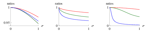
Refer to caption — Fig 1: Graphs of the ratios of $\mathscr{S}_{h,w,\sigma}$ to $K_{w}(h)\sigma^{2}$ for $w=-1$ (left panel), $w=0$ (middle panel), $w=1$ (right panel), $h=\frac{1}{5},1,5$ (red, green, blue — respectively), and $\sigma\in(0,1]$ .

For $w=-1$ , the relative errors are seen to be rather small even for $h$ as large as $5$ and $\sigma$ as large as $1$ . Also, the relative errors appear to be monotonic in $\sigma$ , but not in $h$ or in $w$ .

It is obvious that the upper bounds on $\operatorname{\mathsf{E}}_{h,w}X$ will hold if the factor $X$ of $e^{h(X\wedge w)}$ in the numerator of the ratio in (1.1) is replaced by any r.v. that is no greater than $X$ . Thus, by Theorem 2.4 and Remark 2.2, one has

Corollary 2.7.

Take any $h$ , $w$ , and $\sigma$ in $(0,\infty)$ . Take then any r.v. $X\in\mathscr{X}_{\leqslant\sigma}$ and let $Y$ be any r.v. such that $Y\leqslant X$ with probability $1$ . Then

\frac{\operatorname{\mathsf{E}}Ye^{h(X\wedge w)}}{\operatorname{\mathsf{E}}e^{h(X\wedge w)}}\leqslant\mathscr{S}_{h,w,\sigma}<\frac{e^{hw}-1}{w}\,\sigma^{2}.

In particular, one can take here $Y=X\wedge w$ or $Y=X\operatorname{I}\left\{X\leqslant w\right\}$ .

Remark 2.8.

Suppose that $h$ , $w$ , $\sigma$ , and $X$ are as in Corollary 2.7 and, in addition, $\operatorname{\mathsf{P}}(X\leqslant w)=1$ . Then, by Corollary 2.7,

\frac{\operatorname{\mathsf{E}}Xe^{hX}}{\operatorname{\mathsf{E}}e^{hX}}\leqslant\mathscr{S}_{h,w,\sigma}<\frac{e^{hw}-1}{w}\,\sigma^{2}.

(2.12)

Moreover, according to Theorem 2.4, the bound $\mathscr{S}_{h,w,\sigma}$ on $\frac{\operatorname{\mathsf{E}}Xe^{hX}}{\operatorname{\mathsf{E}}e^{hX}}$ is still exact (even under the additional condition $\operatorname{\mathsf{P}}(X\leqslant w)=1$ ) — provided that $\sigma\leqslant w\sigma_{h}$ ; cf. (2.10). As pointed out before, in the applications that motivated this study, the values of $\sigma$ are typically small and thus will satisfy the condition $\sigma\leqslant w\sigma_{h}$ . Also, the proof of Theorem 2.4 shows (see especially the paragraph containing formula (3.21)) that the factor $\frac{e^{hw}-1}{w}$ in the second upper bound in (2.12) will still be optimal, even under the additional restriction $\sigma\leqslant w\sigma_{h}$ — because the supremum of $\rho_{h,1}(\varepsilon)$ in $\varepsilon\in E_{1}=(0,\infty)$ is “attained” in the limit as $\varepsilon\downarrow 0$ , and, in turn, $\rho_{h,1}(\varepsilon)$ is a supremum in $\sigma$ , which is attained at $\sigma=\sigma_{1}(\varepsilon)=\sqrt{\varepsilon}$ , which latter goes to $0$ as $\varepsilon\downarrow 0$ .

At this point, one is ready to present

2.1 Application: Optimal prior bounds on the Bayes posterior mean for exponential families

Consider a so-called exponential family $\big(p(\cdot|\theta)\big)_{\theta\in\Theta}$ of probability densities on some measurable “data” space $\mathbf{X}$ with respect to some measure on $\mathbf{X}$ ; that is,

p(\mathbf{x}|\theta)=e^{\theta T(\mathbf{x})}c(\theta)q(\mathbf{x})

for some positive Borel-measurable function $c$ on some nonempty Borel-measurable “parameter space” $\Theta\subseteq\mathbb{R}$ , some nonnegative measurable functions $T$ and $q$ on $\mathbf{X}$ , all $\theta\in\Theta$ , and all $\mathbf{x}\in\mathbf{X}$ ; one also needs to require that $p(\mathbf{x}|\theta)$ be measurable in $(\mathbf{x},\theta)$ . Thus, $\theta$ is what is usually referred as the natural parameter. For instance, for the family of the Poisson distributions with parameter $\lambda\in(0,\infty)$ , the natural parameter is $\theta=\ln\lambda\in\mathbb{R}=\Theta$ and $c(\theta)=e^{-\lambda}=e^{-e^{\theta}}$ .

Suppose that $\theta_{\max}:=\sup\Theta<\infty$ . Further, let $\pi$ be a Borel measure on $\Theta$ , which will play the role of a so-called prior distribution. Note that $\pi$ does not have to be a probability distribution. In fact, it will be convenient here to normalize $\pi$ and/or the function $c$ so that $\int_{\Theta}c(\theta)\,\pi(\!\,{\mathrm{d}}\theta)=1$ . Let us exclude the trivial case when $\operatorname{supp}\pi=\{\theta_{\max}\}$ . Then, clearly, $m:=\int_{\Theta}\theta\,c(\theta)\,\pi(\!\,{\mathrm{d}}\theta)<\theta_{\max}$ . Finally, suppose that the variance of the (renormalized by the factor $c$ ) prior distribution is known to be bounded: $\int_{\Theta}(\theta-m)^{2}\,c(\theta)\,\pi(\!\,{\mathrm{d}}\theta)\leqslant\sigma^{2}$ for some $\sigma\in(0,\infty)$ ; such an assumption appears especially reasonable in empirical Bayes settings, when accumulated prior knowledge may greatly reduce the uncertainty about the value of $\theta$ .

Consider now the posterior mean

\hat{\theta}(\mathbf{x}):=\frac{\int_{\Theta}\theta\,p(\mathbf{x}|\theta)\,\pi(\!\,{\mathrm{d}}\theta)}{\int_{\Theta}\,p(\mathbf{x}|\theta)\,\pi(\!\,{\mathrm{d}}\theta)}=\frac{\int_{\Theta}\theta\,e^{\theta t}\,c(\theta)\,\pi(\!\,{\mathrm{d}}\theta)}{\int_{\Theta}\theta\,e^{\theta t}\,c(\theta)\,\pi(\!\,{\mathrm{d}}\theta)}

given some observable “data” $\mathbf{x}\in\mathbf{X}$ (with $q(\mathbf{x})\neq 0$ ), where $t:=T(\mathbf{x})$ . Then, by formula (1.2) and Remarks 2.8 and 2.2, one has

\hat{\theta}(\mathbf{x})-m\leqslant\mathscr{S}_{t,\theta_{\max}-m,\sigma}<\frac{e^{(\theta_{\max}-m)t}-1}{\theta_{\max}-m}\,\sigma^{2},

(2.13)

again for $t=T(\mathbf{x})$ and any $\mathbf{x}\in\mathbf{X}$ (with $q(\mathbf{x})\neq 0$ ). If $\sigma^{2}$ is small enough, then the upper bounds in (2.13) on $\hat{\theta}(\mathbf{x})-m$ may be much smaller than the trivial bound $\theta_{\max}-m$ . Also, by Remark 2.8, the bound $\mathscr{S}_{t,\theta_{\max}-m,\sigma}$ on $\hat{\theta}(\mathbf{x})-m$ is exact, and the factor $\frac{e^{(\theta_{\max}-m)t}-1}{\theta_{\max}-m}$ in the second upper bound in (2.13) is optimal. Recall that the main concern with the Bayesian approach is uncertainty about the choice of the prior distribution. So, the bounds in (2.13) may be of help, as they rely only on the first two moments and an upper bound of the support of such a distribution.

3 Proofs

An approach one could try to use to establish an exact upper bound on the ratio $\operatorname{\mathsf{E}}_{h,w}X$ , defined in (1.1), is to fix — besides the first two moments of $X$ — a value of the denominator, $\operatorname{\mathsf{E}}e^{h(X\wedge w)}$ , and then maximize the numerator, $\operatorname{\mathsf{E}}Xe^{h(X\wedge w)}$ , subject to these three (affine) restrictions on the measure that is the distribution of $X$ . In fact, here one has one more, less explicit restriction on this measure, which can be written as $\operatorname{\mathsf{E}}1=1$ , of course meaning that the measure is a probability one. Then one can use some of well-known results such as those in [4, 6] to reduce the optimization problem to the case when $\operatorname{supp}X$ consists of at most four points, corresponding to the four restrictions on the measure. Then the problem will be reduced to calculus with $12$ variables ( $8$ variables for the four support points of the measure and the four corresponding masses; one variable for the previously fixed value of $\operatorname{\mathsf{E}}e^{h(X\wedge w)}$ ; and also the parameters $h$ , $w$ , and $\sigma$ ). Of these $12$ variables, four can be eliminated using the four restrictions on the measure, and one of the parameters $h,w,\sigma$ can be eliminated by rescaling. Yet, this would leave $7$ variables and a highly nonlinear function to maximize, with a number of restrictions on the variables. Such a problem appears too difficult, in terms of the amount of required calculations, especially symbolic ones.

Here this difficulty is overcome mainly by a thorough exploitation of the duality principle, the idea of which goes back to Chebyshev; see e.g. [krein59, 5, 9, 7, pin-games-transl, 11]. A general expression of this duality is the so-called minimax duality, which goes back to von Neumann [15]; see also e.g. [3, 8, 14, pin-games-transl]; in particular, a necessary and sufficient condition for minimax duality for concave-convex functions was given in [pin-games-transl]. However, more convenient in a number of problems in probability and statistics turn out to be sufficient conditions for duality given by Kemperman [7], which will be used in the present paper as well. Another significant idea in the proof of the basic Theorem 2.1 in this paper is a reduction of the maximization of the ratio $\operatorname{\mathsf{E}}_{h,w}X=\frac{\operatorname{\mathsf{E}}Xe^{h(X\wedge w)}}{\operatorname{\mathsf{E}}e^{h(X\wedge w)}}$ of two affine functions (of the distribution of $X$ ) to the maximization of a linear combination $\operatorname{\mathsf{E}}Xe^{h(X\wedge w)}-k\operatorname{\mathsf{E}}e^{h(X\wedge w)}=\operatorname{\mathsf{E}}(X-k)e^{h(X\wedge w)}$ of these two functions, with an appropriately chosen value of the constant $k$ . As the result, we show that the maximum of $\operatorname{\mathsf{E}}_{h,w}X$ is attained at a r.v. $X$ with $\operatorname{supp}X$ consisting just of two (rather than four) points. This allows for further analysis, to be presented in the proof of Theorem 2.4, resulting in a rather easily computable expression for the maximum of $\operatorname{\mathsf{E}}_{h,w}X$ , as well as simple and explicit, but at the same time optimal, upper bounds on this maximum.

In accordance to some of the above discussion, Theorem 2.1 is obtained as a rather easy corollary of Theorem 3.1 below. To state the latter, let us introduce, for all $k\in\mathbb{R}$ ,

$\displaystyle\mathscr{S}_{k;h,w,\sigma}$	$\displaystyle:=\sup\{\textstyle{\int}_{\mathbb{R}}\,(x-k)e^{h(x\wedge w)}P(\,{\mathrm{d}}x)\colon P\in\mathscr{P}_{\sigma}\}$	(3.1)
	$\displaystyle=\sup\{\operatorname{\mathsf{E}}(X-k)e^{h(X\wedge w)}\colon X\in\mathscr{X}_{\sigma}\},$
$\displaystyle\mathscr{S}_{k;h,w,\leqslant\sigma}$	$\displaystyle:=\sup\{\textstyle{\int}_{\mathbb{R}}\,(x-k)e^{h(x\wedge w)}P(\,{\mathrm{d}}x)\colon P\in\mathscr{P}_{\leqslant\sigma}\}$
	$\displaystyle=\sup\{\operatorname{\mathsf{E}}(X-k)e^{h(X\wedge w)}\colon X\in\mathscr{X}_{\leqslant\sigma}\},$
$\displaystyle\mathscr{S}^{(2)}_{k;h,w,\sigma}$	$\displaystyle:=\sup\{\textstyle{\int}_{\mathbb{R}}\,(x-k)e^{h(x\wedge w)}P(\,{\mathrm{d}}x)\colon P\in\mathscr{P}^{(2)}_{w,\sigma}\}$
	$\displaystyle=\sup\{\operatorname{\mathsf{E}}(X-k)e^{h(X\wedge w)}\colon X\in\mathscr{X}^{(2)}_{w,\sigma}\},$
$\displaystyle\mathscr{S}^{(2)}_{k;h,w,\leqslant\sigma}$	$\displaystyle:=\sup\{\textstyle{\int}_{\mathbb{R}}\,(x-k)e^{h(x\wedge w)}P(\,{\mathrm{d}}x)\colon P\in\mathscr{P}^{(2)}_{w,\leqslant\sigma}\}$
	$\displaystyle=\sup\{\operatorname{\mathsf{E}}(X-k)e^{h(X\wedge w)}\colon X\in\mathscr{X}^{(2)}_{w,\leqslant\sigma}\}.$

Similarly to (2.3), define now the attainment sets $\mathscr{A}_{k;h,w,\sigma}$ , $\mathscr{A}_{k;h,w,\leqslant\sigma}$ , $\mathscr{A}^{(2)}_{k;h,w,\sigma}$ , and $\mathscr{A}^{(2)}_{k;h,w,\leqslant\sigma}$ (as subsets of $\mathscr{P}$ ) for the corresponding suprema in (3.1).

Theorem 3.1.

For any $k\in\mathbb{R}$

(I)

the four suprema in (3.1) are all the same:

\mathscr{S}_{k;h,w,\leqslant\sigma}=\mathscr{S}_{k;h,w,\sigma}=\mathscr{S}^{(2)}_{k;h,w,\sigma}=\mathscr{S}^{(2)}_{k;h,w,\leqslant\sigma};

(3.2)

(II)

each of the four suprema in (3.2) is (strictly) increasing in $\sigma\in(0,\infty)$ ;

(III)

each of these suprema is attained, and

\mathscr{A}_{k;h,w,\leqslant\sigma}=\mathscr{A}_{k;h,w,\sigma}=\mathscr{A}^{(2)}_{k;h,w,\sigma}=\mathscr{A}^{(2)}_{k;h,w,\leqslant\sigma}.

(3.3)

Proof of Theorem 2.1 (modulo Theorem 3.1).

Note first that all the four suprema in (2.4) are finite, because $\mathscr{X}^{(2)}_{w,\sigma}\neq\emptyset$ and, for any r.v. $X\in\mathscr{X}_{\leqslant\sigma}$ , one has $|\operatorname{\mathsf{E}}Xe^{h(X\wedge w)}|\leqslant\operatorname{\mathsf{E}}|X|e^{hw}\leqslant\sigma e^{h|w|}$ , $\operatorname{\mathsf{E}}e^{h(X\wedge w)}\geqslant e^{h\operatorname{\mathsf{E}}(X\wedge w)}\geqslant e^{-h(\operatorname{\mathsf{E}}|X|+|w|)}\geqslant e^{-h(\sigma+|w|)}$ , and hence $|\operatorname{\mathsf{E}}_{h,w}X|\leqslant\sigma e^{h(\sigma+2|w|)}$ . If now $k$ is chosen to coincide with $\mathscr{S}^{(2)}_{h,w,\sigma}$ , then

\operatorname{\mathsf{E}}(X-k)e^{h(X\wedge w)}=(\operatorname{\mathsf{E}}_{h,w}X-k)\operatorname{\mathsf{E}}e^{h(X\wedge w)}\leqslant 0

(3.4)

for all $X\in\mathscr{X}^{(2)}_{w,\sigma}$ , so that $\mathscr{S}^{(2)}_{k;h,w,\sigma}\leqslant 0$ ; in fact, $\mathscr{S}^{(2)}_{k;h,w,\sigma}=0$ , since the factor $\operatorname{\mathsf{E}}e^{h(X\wedge w)}$ stays between $0$ and $e^{hw}$ , and hence is bounded. So, by Theorem 3.1, $\mathscr{S}_{k;h,w,\sigma}=0$ . Therefore,

\operatorname{\mathsf{E}}Xe^{h(X\wedge w)}\leqslant k\operatorname{\mathsf{E}}e^{h(X\wedge w)}

(3.5)

for all $X\in\mathscr{X}_{\sigma}$ , which implies that $\mathscr{S}_{h,w,\sigma}\leqslant k=\mathscr{S}^{(2)}_{h,w,\sigma}$ . The reverse inequality, $\mathscr{S}_{h,w,\sigma}\geqslant\mathscr{S}^{(2)}_{h,w,\sigma}$ , is trivial. So, the second equality in (2.4) is verified. Moreover, by Theorem 3.1, the supremum $\mathscr{S}^{(2)}_{k;h,w,\sigma}=0$ is attained at some r.v. $X\in\mathscr{X}^{(2)}_{w,\sigma}$ , for which inequality (3.5) must then turn into the equality $\operatorname{\mathsf{E}}Xe^{h(X\wedge w)}=k\operatorname{\mathsf{E}}e^{h(X\wedge w)}$ , which is equivalent to $\operatorname{\mathsf{E}}_{h,w}X=k$ . So, the suprema $\mathscr{S}^{(2)}_{h,w,\sigma}$ and $\mathscr{S}_{h,w,\sigma}$ are attained.

Let us now verify the monotonicity of $\mathscr{S}_{h,w,\sigma}(=\mathscr{S}^{(2)}_{h,w,\sigma})$ in $\sigma\in(0,\infty)$ (which will also yield the first and third equalities in (2.4), as well as the attainment of the suprema $\mathscr{S}_{h,w,\leqslant\sigma}$ and $\mathscr{S}^{(2)}_{h,w,\leqslant\sigma}$ ). Here the reasoning is similar to that in the previous paragraph, again with $k=\mathscr{S}^{(2)}_{h,w,\sigma}$ , which, as was shown, equas to $\mathscr{S}_{h,w,\sigma}$ . Then relations (3.4) hold for all $X\in\mathscr{X}_{\sigma}$ , so that $\mathscr{S}_{k;h,w,\sigma}=0$ . Take now any $\sigma_{1}\in(0,\sigma)$ . Then, by part (II) of Theorem 3.1, $\mathscr{S}_{k;h,w,\sigma_{1}}<\mathscr{S}_{k;h,w,\sigma}=0$ . Again using the equality in (3.4) (with its two sides interchanged), one has $\operatorname{\mathsf{E}}_{h,w}X<k=\mathscr{S}_{h,w,\sigma}$ for all $X\in\mathscr{X}_{\sigma_{1}}$ , which implies $\mathscr{S}_{h,w,\sigma_{1}}<\mathscr{S}_{h,w,\sigma}$ — since, by what has been already proved, the supremum $\mathscr{S}_{h,w,\sigma_{1}}$ is attained at some $X\in\mathscr{X}_{\sigma_{1}}$ .

It remains to observe that (2.5) follows from (3.3). Indeed, for any $P_{*}\in\mathscr{P}$ , one has $P_{*}\in\mathscr{A}_{h,w,\sigma}$ if and only if $P_{*}\in\mathscr{A}_{k;h,w,\sigma}$ for $k=\mathscr{S}_{h,w,\sigma}$ and at that $\mathscr{S}_{k;h,w,\sigma}=0$ ; and the same is true for each of the pairs of the subscript/superscript attributes $({}_{h,w,\leqslant\sigma},\;{}_{k;h,w,\leqslant\sigma})$ , $({}^{(2)}_{h,w,\sigma},\;{}^{(2)}_{k;h,w,\sigma})$ , $({}^{(2)}_{h,w,\leqslant\sigma},\;{}^{(2)}_{k;h,w,\leqslant\sigma})$ in place of the pair $({}_{h,w,\sigma},\;{}_{k;h,w,\sigma})$ . ∎

Proof of Theorem 3.1.

Introduce more notation. First, let $S$ stand for the set $[-\infty,\infty]$ , equipped with the natural topology and the corresponding Borel sigma-algebra; then $S$ is compact. Next, take indeed any $k\in\mathbb{R}$ and define the real-valued functions $a_{1},a_{2},a_{3},b$ on $S$ by the formulas

a_{j}(s):=\frac{s^{j-1}}{1+s^{2}}\quad\text{and}\quad b(s):=\frac{(s-k)e^{h(s\wedge w)}}{1+s^{2}}

for all $j\in\{1,2,3\}$ and $s\in\mathbb{R}$ (assuming the convention $0^{0}:=1$ ), with the values of these functions on the set $\{-\infty,\infty\}$ defined by continuity, so that $a_{j}(\pm\infty)=b(\pm\infty)=0$ for $j\in\{1,2\}$ and $a_{3}(\pm\infty)=1$ .

Further, let $\mathscr{M}$ stand for the set of all (nonnegative) Borel measures on $S$ . Introduce now the sets

$\displaystyle A:=$	$\displaystyle\big\{\big(\textstyle{\int}a_{1}\,{\mathrm{d}}\mu,\textstyle{\int}a_{2}\,{\mathrm{d}}\mu,\textstyle{\int}a_{2}\,{\mathrm{d}}\mu\big)\in\mathbb{R}^{3}\colon\mu\in\mathscr{M},\$
	$\displaystyle\hskip 142.26378pt\textstyle{\int}(\|a_{1}\|+\|a_{2}\|+\|a_{3}\|)\,{\mathrm{d}}\mu<\infty\big\},$
$\displaystyle\mathscr{M}_{\sigma}:=$	$\displaystyle\big\{\mu\in\mathscr{M}\colon\big(\textstyle{\int}a_{1}\,{\mathrm{d}}\mu,\textstyle{\int}a_{2}\,{\mathrm{d}}\mu,\textstyle{\int}a_{2}\,{\mathrm{d}}\mu\big)=(1,0,\sigma^{2})\big\},$
$\displaystyle C:=$	$\displaystyle\big\{(c_{1},c_{2},c_{3})\in\mathbb{R}^{3}\colon c_{1}a_{1}(s)+c_{2}a_{2}(s)+c_{3}a_{3}(s)\geqslant b(s)\text{ for all }s\in S\big\},$	(3.6)

where the integrals are over $S$ . Also, let

\displaystyle B(c_{1},c_{2},c_{3}):=

\displaystyle\{s\in S\colon c_{1}a_{1}(s)+c_{2}a_{2}(s)+c_{3}a_{3}(s)=b(s)\};

(3.7)

for $(c_{1},c_{2},c_{3})\in C$ , the set $B(c_{1},c_{2},c_{3})$ is sometimes referred to as the contact set — compare (3.6) and (3.7).

Observe the following.

•

For all $\mu\in\mathscr{M}_{\sigma}$ , one has $\textstyle{\int}|b|\,{\mathrm{d}}\mu<\infty$ , since $|b|=O(a_{1}+a_{3})$ . For the same reason, $C\neq\emptyset$ . Moreover, the strict inequality $ca_{1}+ca_{3}>b$ holds (on $S$ ) for some large enough $c\in(0,\infty)$ (depending on $h$ and $k$ ).
•

The point $(1,0,\sigma^{2})$ lies in the interior of the set $A\subseteq\mathbb{R}^{3}$ . This follows because the condition $\sigma\in(0,\infty)$ implies that (i) there is a measure $\mu\in\mathscr{M}_{\sigma}$ with $\operatorname{card}\,\operatorname{supp}\mu=3$ and (ii) the restrictions of the functions $a_{1},a_{2},a_{3}$ to the three-point set $\operatorname{supp}\mu$ are linearly independent.

(As usual, $\operatorname{card}$ denotes the cardinality.) Therefore, by Theorems 3 and 4 in [7] (see also comments in the penultimate paragraph of [7, Section 3]), there exist $(c^{\circ}_{1},c^{\circ}_{2},c^{\circ}_{3})\in C$ and $\mu^{\circ}\in\mathscr{M}_{\sigma}$ such that

\operatorname{supp}\mu^{\circ}\subseteq B(c^{\circ}_{1},c^{\circ}_{2},c^{\circ}_{3})\quad\text{and}\quad\sup\{\textstyle{\int}b\,{\mathrm{d}}\mu\colon\mu\in\mathscr{M}_{\sigma}\}=\textstyle{\int}b\,{\mathrm{d}}\mu^{\circ}.

(3.8)

Moreover, the conditions $\sigma\in(0,\infty)$ and $\mu^{\circ}\in\mathscr{M}_{\sigma}$ imply that $\operatorname{card}\operatorname{supp}\mu^{\circ}\geqslant 2$ . So, by Lemma 3.2 below,

\operatorname{supp}\mu^{\circ}=\{-u,v\}

(3.9)

for some real numbers $u$ and $v$ such that $-u<w\leqslant v$ ; in particular, $\operatorname{supp}\mu^{\circ}\subseteq\mathbb{R}$ .

Next, observe that the formula

P(\,{\mathrm{d}}s)=\frac{\mu(\,{\mathrm{d}}s)}{1+s^{2}}

(3.10)

defines a one-to-one correspondence between the set $\{\mu\in\mathscr{M}_{\sigma}\colon\operatorname{supp}\mu\subseteq\mathbb{R}\}$ and the set $\mathscr{P}_{\sigma}$ of zero-mean probability measures on $\mathbb{R}$ , defined in (2.1) (the formal meaning of (3.10) is of course that the Radon–Nikodym derivative of $P$ relative to $\mu$ is the function $s\mapsto\frac{1}{1+s^{2}}$ ). Moreover, for any so-related measures $\mu$ and $P$ , one has $\int_{S}b\,{\mathrm{d}}\mu=\int_{\mathbb{R}}(x-k)e^{h(x\wedge w)}P(\,{\mathrm{d}}x)$ . Now, in view of (3.8) and (3.1),

$\displaystyle\mathscr{S}_{k;h,w,\sigma}=$	$\displaystyle\sup\{\textstyle{\int}_{\mathbb{R}}\,(x-k)e^{h(x\wedge w)}P(\,{\mathrm{d}}x)\colon P\in\mathscr{P}_{\sigma}\}$	(3.11)
$\displaystyle=$	$\displaystyle\sup\{\textstyle{\int}_{S}\,b\,{\mathrm{d}}\mu\colon\mu\in\mathscr{M}_{\sigma},\;\operatorname{supp}\mu\subseteq\mathbb{R}\}$
$\displaystyle\leqslant$	$\displaystyle\sup\{\textstyle{\int}_{S}\,b\,{\mathrm{d}}\mu\colon\mu\in\mathscr{M}_{\sigma}\}$
$\displaystyle=$	$\displaystyle{\textstyle\displaystyle\int}_{S}\,b\,{\mathrm{d}}\mu^{\circ}$
$\displaystyle=$	$\displaystyle{\textstyle\displaystyle\int}_{\mathbb{R}}\,(x-k)e^{h(x\wedge w)}P^{\circ}(\,{\mathrm{d}}x)\leqslant\mathscr{S}^{(2)}_{k;h,w,\sigma}\leqslant\mathscr{S}_{k;h,w,\sigma},$

where $P^{\circ}$ is the measure corresponding to $\mu^{\circ}$ by means of (3.10), so that, by (3.9), $P^{\circ}\in\mathscr{P}^{(2)}_{w,\sigma}\subseteq\mathscr{P}_{\sigma}$ . Thus, both suprema $\mathscr{S}_{k;h,w,\sigma}$ and $\mathscr{S}^{(2)}_{k;h,w,\sigma}$ are attained at $P=P^{\circ}$ and are equal to each other, so that the second equality in (3.2) holds.

Next, let us prove the monotonicity of $\mathscr{S}_{k;h,w,\sigma}(=\mathscr{S}^{(2)}_{k;h,w,\sigma})$ in $\sigma\in(0,\infty)$ , which will also yield the first and third equalities in (3.2), as well as the attainment of the suprema $\mathscr{S}_{k;h,w,\leqslant\sigma}$ and $\mathscr{S}^{(2)}_{k;h,w,\leqslant\sigma}$ . Take any $\sigma_{1}\in(0,\sigma)$ and then take any $P\in\mathscr{P}_{\sigma_{1}}$ .

Let now the measure $\mu\in\mathscr{M}_{\sigma_{1}}$ with $\operatorname{supp}\mu\subseteq\mathbb{R}$ be defined by the formula $\mu(\,{\mathrm{d}}s)=(1+s^{2})P(\,{\mathrm{d}}s)$ , in accordance with the correspondence (3.10). It follows that

\textstyle{\int}_{\mathbb{R}}\,(x-k)e^{h(x\wedge w)}P(\,{\mathrm{d}}x)=\textstyle{\int}b\,{\mathrm{d}}\mu\leqslant\int(c^{\circ}_{1}a_{1}+c^{\circ}_{2}a_{2}+c^{\circ}_{3}a_{3})\,{\mathrm{d}}\mu=c^{\circ}_{1}+c^{\circ}_{3}\sigma_{1}^{2}\\ <c^{\circ}_{1}+c^{\circ}_{3}\sigma^{2}=\textstyle{\int}b\,{\mathrm{d}}\mu^{\circ}=\mathscr{S}_{k;h,w,\sigma};

(3.12)

here,

•

the first equality follows by the definition of $\mu$ ;
•

the first inequality, by the condition $(c^{\circ}_{1},c^{\circ}_{2},c^{\circ}_{3})\in C$ ;
•

the second equality, because $\mu\in\mathscr{M}_{\sigma_{1}}$ ;
•

the second inequality — because, by Lemma 3.2 below, the condition $(c^{\circ}_{1},c^{\circ}_{2},c^{\circ}_{3})\in C$ implies $c^{\circ}_{3}>0$ , while $\sigma_{1}^{2}<\sigma^{2}$ ;
•

the third equality, because $\mu^{\circ}\in\mathscr{M}_{\sigma}$ ;
•

the last equality, by (3.11).

Now one can see that $\mathscr{S}_{k;h,w,\sigma_{1}}\leqslant\mathscr{S}_{k;h,w,\sigma}$ ; moreover, this latter inequality is strict, since the last inequality in (3.12) is strict and, by what was already proved, the supremum $\mathscr{S}_{k;h,w,\sigma_{1}}$ is attained. This concludes the proof of parts (I) and (II) of Theorem 3.1 — modulo Lemma 3.2.

Next, let us prove (3.3). First here, note that the obvious relation $\mathscr{P}_{\sigma}\subseteq\mathscr{P}_{\leqslant\sigma}$ , together with (3.2), implies $\mathscr{A}_{k:h,w,\sigma}\leqslant\mathscr{A}_{k:h,w,\leqslant\sigma}$ , and the reverse inequality follows by the already checked strict monotonicity of $\mathscr{S}_{k;h,w,\sigma}$ in $\sigma$ . So, one has the first equality in (3.3), and the third equality there is verified similarly.

To obtain a contradiction, suppose now that the second equality in (3.3) is false, so that there exists some $P_{*}\in\mathscr{A}_{k;h,w,\sigma}\setminus\mathscr{A}^{(2)}_{k;h,w,\sigma}$ . Then, again by Lemma 3.2, the set $S^{\circ}:=\operatorname{supp}\mu_{*}\setminus B(c^{\circ}_{1},c^{\circ}_{2},c^{\circ}_{3})$ is nonempty, where $\mu_{*}\in\mathscr{M}_{\sigma}$ is the measure corresponding to $P_{*}$ in accordance with the correspondence (3.10) and $(c^{\circ}_{1},c^{\circ}_{2},c^{\circ}_{3})\in C$ is as before; moreover, the condition $\operatorname{supp}\mu_{*}\not\subseteq B(c^{\circ}_{1},c^{\circ}_{2},c^{\circ}_{3})$ implies $\mu_{*}(S^{\circ})>0$ , because the functions $a_{1}$ , $a_{2}$ , $a_{3}$ , and $b$ are continuous and hence the set $B(c^{\circ}_{1},c^{\circ}_{2},c^{\circ}_{3})$ is closed. So and because $c^{\circ}_{1}a_{1}+c^{\circ}_{2}a_{2}+c^{\circ}_{3}a_{3}\geqslant b$ on $S$ and $c^{\circ}_{1}a_{1}+c^{\circ}_{2}a_{2}+c^{\circ}_{3}a_{3}>b$ on $S^{\circ}$ , it follows that

\textstyle{\int}(c^{\circ}_{1}a_{1}+c^{\circ}_{2}a_{2}+c^{\circ}_{3}a_{3}-b)\,{\mathrm{d}}\mu_{*}\geqslant\textstyle{\int}_{\!S^{\circ}}\,(c^{\circ}_{1}a_{1}+c^{\circ}_{2}a_{2}+c^{\circ}_{3}a_{3}-b)\,{\mathrm{d}}\mu_{*}>0.

(3.13)

Now one can write

\mathscr{S}_{k;h,w,\sigma}=\textstyle{\int}b\,{\mathrm{d}}\mu_{*}<\textstyle{\int}(c^{\circ}_{1}a_{1}+c^{\circ}_{2}a_{2}+c^{\circ}_{3}a_{3})\,{\mathrm{d}}\mu_{*}=\textstyle{\int}(c^{\circ}_{1}a_{1}+c^{\circ}_{2}a_{2}+c^{\circ}_{3}a_{3})\,{\mathrm{d}}\mu^{\circ}\\ =\textstyle{\int}b\,{\mathrm{d}}\mu^{\circ}=\mathscr{S}_{k;h,w,\sigma},

which is indeed a contradiction; the first equality here follows by the condition $P_{*}\in\mathscr{A}_{k;h,w,\sigma}$ , the first inequality, by (3.13); the second equality, because $\mu_{*}$ and $\mu^{\circ}$ are in $\mathscr{M}_{\sigma}$ ; the penultimate equality, since $\operatorname{supp}\mu^{\circ}\subseteq B(c^{\circ}_{1},c^{\circ}_{2},c^{\circ}_{3})$ ; and the last equality, by (3.11).

Thus, to complete the proof of Theorem 3.1, it remains to verify

Lemma 3.2.

For any $(c_{1},c_{2},c_{3})\in C$ , one has $c_{3}>0$ and, moreover, the set $B(c_{1},c_{2},c_{3})$ is empty, a singleton, or of the form $\{-u,v\}$ for some real numbers $u$ and $v$ such that $-u<w\leqslant v$ ; so, in all cases $\operatorname{card}B(c_{1},c_{2},c_{3})\leqslant 2$ .

Proof of Lemma 3.2.

Take any $(c_{1},c_{2},c_{3})\in C$ , so that, by (3.6),

\displaystyle d(s):=c_{1}a_{1}(s)+c_{2}a_{2}(s)+c_{3}a_{3}(s)-b(s)\geqslant 0

(3.14)

for all $s\in S=[-\infty,\infty]$ and, by (3.7),

B(c_{1},c_{2},c_{3})=\{s\in S\colon d(s)=0\}.

(3.15)

Since $d(\infty)=c_{3}$ , inequality (3.14) implies that $c_{3}\geqslant 0$ . Moreover, if $c_{3}=0$ , then $s\,d(s)\to c_{2}-e^{h}$ as $s\to\infty$ and $s\,d(s)\to c_{2}$ as $s\to-\infty$ , whence $e^{h}\leqslant c_{2}\leqslant 0$ , which is a contradiction. We conclude that indeed

c_{3}>0.

(3.16)

In turn, this implies that $d(s)=c_{3}\neq 0$ for $s\in\{-\infty,\infty\}$ . Therefore, by (3.15), $B(c_{1},c_{2},c_{3})\cap\{-\infty,\infty\}=\emptyset$ , so that

	$\displaystyle B(c_{1},c_{2},c_{3})=\{s\in\mathbb{R}\colon\tilde{d}(s)=0\},\quad\text{where}$
	$\displaystyle\tilde{d}(s):=d(s)(1+s^{2})=c_{1}+c_{2}s+c_{3}s^{2}-(s-k)e^{h(s\wedge w)}.$

Next, observe that the restriction of the function $\tilde{d}$ to the interval $[w,\infty)$ is strictly convex (as a quadratic polynomial with the leading coefficient $c_{3}>0$ ) and hence

\operatorname{card}\big(B(c_{1},c_{2},c_{3})\cap[w,\infty)\big)\leqslant 1.

It remains to show that

\operatorname{card}\big(B(c_{1},c_{2},c_{3})\cap(-\infty,w)\big)\leqslant 1.

Assume the contrary, so that there exist real numbers $u$ and $v$ in $B(c_{1},c_{2},c_{3})$ such that $u<v<w$ . Since the function $\tilde{d}$ is differentiable on $(-\infty,w)$ , it follows that

\tilde{d}(u)=\tilde{d}^{\prime}(u)=\tilde{d}(v)=\tilde{d}^{\prime}(v)=0.

The latter equalities constitute a system of four linear equations in $c_{1},c_{2},c_{3},k$ . Solving it, one finds that, in particular,

c_{3}=\frac{he^{hu}}{\delta}\,\frac{\operatorname{num}}{\operatorname{den}},

where $\operatorname{num}:=\delta^{2}-4\sinh^{2}\frac{\delta}{2}$ , $\operatorname{den}:=\delta-2+(\delta+2)e^{-\delta}$ , and $\delta:=h(v-u)>0$ . It is easy to see that $\operatorname{num}<0<\operatorname{den}$ for any $\delta\in(0,\infty)$ , which implies $c_{3}<0$ and thus contradicts (3.16). Now Lemma 3.2 is completely proved, and thus so is Theorem 3.1. ∎

∎

Proof of Proposition 2.3.

For $\varepsilon\in(0,\infty)$ , introduce

\delta(\varepsilon):=\delta_{h}(\varepsilon):=\frac{u_{*}(h,\varepsilon)-\varepsilon}{\varepsilon^{2}e^{2(1+\varepsilon)h}}\,\big(e^{(1+\varepsilon)h}(1+\varepsilon h)-1\big);

then $u_{*}(h,\varepsilon)-\varepsilon\overset{\operatorname{sign}}{=}\delta(\varepsilon)$ , $\delta^{\prime}(\varepsilon)\overset{\operatorname{sign}}{=}e^{(1+\varepsilon)h}(1+\varepsilon h+\varepsilon^{2}(1+\varepsilon)h^{2})-(1+2\varepsilon h)>(1+\varepsilon h)^{2}-(1+2\varepsilon h)>0$ , so that the continuous function $\delta$ is (strictly) increasing, from $\delta(0+)=-\infty$ to $\delta(\infty-)=1$ . Now part (i) of Proposition 2.3 follows.

It also follows that $u_{*}(h,\varepsilon)-\varepsilon\overset{\operatorname{sign}}{=}\varepsilon-\sigma_{h}^{2}$ for all $\varepsilon\in(0,\infty)$ , so that $u_{*}(h,\sigma^{2})>\sigma^{2}$ — assuming the condition $\sigma>\sigma_{h}$ of part (ii) of Proposition 2.3. Since $u_{*}(h,\varepsilon)$ is continuous in $\varepsilon\in(0,\infty)$ , with $u_{*}(h,0+)=0$ , to complete the proof of part (ii) of the proposition it remains to note that $u_{*}(h,\varepsilon)$ is increasing in $\varepsilon\in(0,\infty)$ , which follows because, with $z:=\varepsilon h$ ,

	$\displaystyle\frac{\partial u_{*}(h,\varepsilon)}{\partial\varepsilon}\,\frac{\big(1+\varepsilon h-e^{-(1+\varepsilon)h}\big)^{2}}{(1-e^{-(1+\varepsilon)h})\,\varepsilon}=$	$\displaystyle(z^{2}+2z+2)e^{(1+1/\varepsilon)z}-z^{2}-4z-2$
	$\displaystyle>$	$\displaystyle(z^{2}+2z+2)(1+z)-z^{2}-4z-2>0.$

Consider next part (iii) of Proposition 2.3. Take here indeed any $w\in\{-1,0\}$ . Then

	$\displaystyle r^{\prime}_{w,1}(\varepsilon)$	$\displaystyle\overset{\operatorname{sign}}{=}r_{w,2}(\varepsilon):=1-\frac{2\varepsilon e^{(\varepsilon+w)h}(1+\varepsilon h)}{\varepsilon^{3}h^{2}+\left(h^{2}\sigma^{2}+2\right)\varepsilon+2h\sigma^{2}+4\varepsilon^{2}h},$
	$\displaystyle r^{\prime}_{w,2}(\varepsilon)$	$\displaystyle\overset{\operatorname{sign}}{=}-\varepsilon^{3}h^{3}\left(\sigma^{2}+\varepsilon^{2}\right)-4\varepsilon^{2}h^{2}\left(\sigma^{2}+\varepsilon^{2}\right)-2\left(2\varepsilon^{3}+3\sigma^{2}\varepsilon\right)h-2\sigma^{2},$

which is manifestly negative for all $\varepsilon\in(|w|,\infty)$ . So, $r_{w,2}(\varepsilon)$ decreases from $r_{w,2}(|w|+)=\frac{h\left(\sigma^{2}+|w|^{2}\right)(h|w|+2)}{2h\sigma^{2}+h^{2}|w|^{3}+|w|\left(h^{2}\sigma^{2}+2\right)+4h|w|^{2}}>0$ to $r_{w,2}(\infty-)=-\infty<0$ as $\varepsilon$ increases from $|w|$ to $\infty$ . Therefore, $r_{w,1}(\varepsilon)$ switches (just once) from increase to decrease as $\varepsilon$ increases from $|w|$ to $\infty$ . Since $r_{w,1}(|w|+)=h|w|(w^{2}+\sigma^{2})\geqslant 0$ and $r_{w,1}(\infty-)=-\infty<0$ , one sees that $r_{w,1}(\varepsilon)$ switches (just once) in sign from $+$ to $-$ as $\varepsilon$ increases from $|w|$ to $\infty$ . This verifies part (iii) of the proposition. Now Proposition 2.3 is completely proved. ∎

Proof of Theorem 2.4.

Take indeed any $w\in\{-1,0,1\}$ . Introduce

	$\displaystyle\Pi_{w}$	$\displaystyle:=\{(\varepsilon,\sigma)\in(0,\infty)^{2}\colon-\varepsilon<w\leqslant\sigma^{2}/\varepsilon\},$
	$\displaystyle E_{w}$	$\displaystyle:=\{\varepsilon\in(0,\infty)\colon(\varepsilon,\sigma)\in\Pi_{w}\text{ for some }\sigma\in(0,\infty)\}$
		$\displaystyle=\big(0\vee(-w),\infty\big),$
	$\displaystyle E_{w,\sigma}$	$\displaystyle:=\{\varepsilon\in(0,\infty)\colon(\varepsilon,\sigma)\in\Pi_{w}\}=\left\{\begin{aligned} &(0,\sigma^{2}]&\text{ if }&w=1,\\ &(-w,\infty)&\text{ if }&w\in\{-1,0\}\end{aligned}\right.$
for all $\sigma\in(0,\infty)$ ,
	$\displaystyle\Sigma_{w,\varepsilon}$	$\displaystyle:=\{\sigma\in(0,\infty)\colon(\varepsilon,\sigma)\in\Pi_{w}\}=\left\{\begin{aligned} &[\sqrt{\varepsilon},\infty)&\text{ if }&w=1,\\ &(0,\infty)&\text{ if }&w\in\{-1,0\}\end{aligned}\right.$
for all $\varepsilon\in E_{w}$ ,
	$\displaystyle m_{w}(\varepsilon)$	$\displaystyle:=m_{w,\sigma}(\varepsilon):=m_{h,w,\sigma}(\varepsilon):=\operatorname{\mathsf{M}}_{h,w}P_{\varepsilon,\,\sigma^{2}/\varepsilon}=\varepsilon\sigma^{2}\,\frac{e^{hw}-e^{-\varepsilon h}}{\varepsilon^{2}e^{hw}+\sigma^{2}e^{-\varepsilon h}}$	(3.17)

for all $(\varepsilon,\sigma)\in\Pi_{w}$ . By Theorem 2.1,

\displaystyle\mathscr{S}_{h,w,\sigma}=\max_{\varepsilon\in E_{w,\sigma}}m_{h,w,\sigma}(\varepsilon).

So, (2.9) and the equality in (2.11) will follow once it is shown that

\argmax\limits_{\varepsilon\in E_{w,\sigma}}m_{h,w,\sigma}(\varepsilon)\overset{\text{(?)}}{=}\{\varepsilon_{h,w,\sigma}\}.

(3.18)

Consider first the case $w=1$ . Recalling the definition (2.6) of $u_{*}(h,\varepsilon)$ and using Proposition 2.3, one has

m^{\prime}_{1}(\varepsilon)\overset{\operatorname{sign}}{=}\sigma^{2}-u_{*}(h,\varepsilon)\overset{\operatorname{sign}}{=}\tilde{\varepsilon}_{h,\sigma}-\varepsilon

(3.19)

for all $\varepsilon\in E_{1,\sigma}=(0,\sigma^{2}]$ , where $m^{\prime}_{1}$ stands for the left-hand side derivative of $m_{1}$ . So, $m_{1}(\varepsilon)$ is increasing in $\varepsilon\in(0,\tilde{\varepsilon}_{h,\sigma}]$ and decreasing in $\varepsilon\in[\tilde{\varepsilon}_{h,\sigma},\infty)\cap(0,\sigma^{2}]$ . Also, it was shown in the proof of Proposition 2.3 that (i) $u_{*}(h,\varepsilon)$ is increasing (from $0$ ) in $\varepsilon\in(0,\infty)$ and (ii) $u_{*}(h,\varepsilon)-\varepsilon\overset{\operatorname{sign}}{=}\varepsilon-\sigma_{h}^{2}$ for all $\varepsilon\in(0,\infty)$ . So, $\sigma^{2}-u_{*}(h,\varepsilon)$ is decreasing in $\varepsilon\in(0,\sigma^{2}]$ from $\sigma^{2}>0$ to $\sigma^{2}-u_{*}(h,\sigma^{2})\overset{\operatorname{sign}}{=}\sigma_{h}^{2}-\sigma^{2}\overset{\operatorname{sign}}{=}\sigma_{h}-\sigma$ . Hence, by (3.19), in the case $\sigma\leqslant\sigma_{h}$ one has $m_{1}^{\prime}(\varepsilon)>0$ for all $\varepsilon\in(0,\sigma^{2}]$ , so that the maximum of $m_{1}(\varepsilon)$ in $\varepsilon\in(0,\sigma^{2}]$ is attained only at $\varepsilon=\sigma^{2}=\varepsilon_{h,1,\sigma}$ , by (2.10). Similarly, in the case $\sigma>\sigma_{h}$ the sign of $m_{1}^{\prime}(\varepsilon)$ changes only at the point $\tilde{\varepsilon}_{h,\sigma}$ , from $+$ to $-$ , as $\varepsilon$ increases from $0$ to $\sigma^{2}$ , so that the maximum of $m_{1}(\varepsilon)$ in $\varepsilon\in(0,\sigma^{2}]$ is in this case attained only at $\varepsilon=\tilde{\varepsilon}_{h,\sigma}=\varepsilon_{h,1,\sigma}$ . This verifies (3.18) for $w=1$ .

The case $w\in\{-1,0\}$ is simpler. Indeed, then $m^{\prime}_{w}(\varepsilon)\overset{\operatorname{sign}}{=}r_{w,1}(\varepsilon)$ for all $\varepsilon\in E_{w,\sigma}$ , where $r_{w,1}(\varepsilon)$ is as in (2.8). Also, as shown at the end of the proof of Proposition 2.3, $r_{w,1}(\varepsilon)$ switches (just once, at $\varepsilon=\varepsilon_{h,w,\sigma}$ ) in sign from $+$ to $-$ as $\varepsilon$ increases from $|w|$ to $\infty$ , for each $w\in\{-1,0\}$ ). So, one has (3.18) for $w\in\{-1,0\}$ as well. This proves (2.9) and the equality (2.11) for all $w\in\{-1,0,1\}$ .

It remains to show that the inequality in (2.11) holds and the constant factor $K_{w}(h)$ therein is the best possible. Introduce

r_{h,w,\sigma}(\varepsilon):=\frac{m_{h,w,\sigma}(\varepsilon)}{\sigma^{2}}=\varepsilon\,\frac{e^{hw}-e^{-\varepsilon h}}{\varepsilon^{2}e^{hw}+\sigma^{2}e^{-\varepsilon h}}

for all $(\varepsilon,\sigma)\in\Pi_{w}$ , by (3.17). Next, observe that $r_{h,w,\sigma}(\varepsilon)$ strictly decreases in $\sigma\in\Sigma_{w,\varepsilon}$ ; here and in what follows, it is assumed by default that $\varepsilon\in E_{w}$ . So,

$\displaystyle\rho_{h,w}(\varepsilon)$	$\displaystyle:=\sup\Big\{\frac{m_{h,w,\sigma}(\varepsilon)}{\sigma^{2}}\colon\sigma\in\Sigma_{w,\varepsilon}\Big\}$	(3.20)
	$\displaystyle=\sup\{r_{h,w,\sigma}(\varepsilon)\colon\sigma\in\Sigma_{w,\varepsilon}\}=r_{h,w,\sigma_{w}(\varepsilon)}(\varepsilon),\quad\text{where}$
$\displaystyle\sigma_{w}(\varepsilon)$	$\displaystyle:=\inf\Sigma_{w,\varepsilon}=(w\vee 0)\sqrt{\varepsilon}.$

Consider now the case $w=1$ , so that $E_{w}=E_{1}=(0,\infty)$ , $\sigma_{w}(\varepsilon)=\sigma_{1}(\varepsilon)=\sqrt{\varepsilon}$ , and

\rho_{h,w}(\varepsilon)=\rho_{h,1}(\varepsilon)=r_{h,1,\sqrt{\varepsilon}}(\varepsilon)=\frac{e^{(1+\varepsilon)h}-1}{1+\varepsilon e^{(1+\varepsilon)h}}.

(3.21)

Now note that $\rho_{h,1}^{\prime}(\varepsilon)\overset{\operatorname{sign}}{=}1+(1+\varepsilon)h-e^{(1+\varepsilon)h}<0$ . Hence, $\rho_{h,1}(\varepsilon)<\rho_{h,1}(0+)=e^{h}-1=K_{1}(h)$ , which, together with (3.17) and (3.20), shows that the inequality in (2.11) holds and that the constant factor $K_{1}(h)$ there is the best possible — in the case $w=1$ .

Next, consider the case $w\in\{-1,0\}$ , when $E_{w}=(-w,\infty)$ , $\sigma_{w}(\varepsilon)=0$ , and

r_{h,w,\sigma}(\varepsilon)<r_{h,w,0+}(\varepsilon)=\rho_{h,w}(\varepsilon)=\frac{1-e^{-(w+\varepsilon)h}}{\varepsilon}

(3.22)

for all $\sigma\in\Sigma_{w,\varepsilon}=(0,\infty)$ . On the other hand, with

u:=-(1+\varepsilon h),

one has

	$\displaystyle\rho^{\prime}_{h,w}(\varepsilon)\overset{\operatorname{sign}}{=}(1+\varepsilon h)e^{-(w+\varepsilon)h}-1\overset{\operatorname{sign}}{=}-ue^{u}-e^{hw-1}$	$\displaystyle\overset{\operatorname{sign}}{=}u-L_{-1}(-e^{hw-1})$
		$\displaystyle\overset{\operatorname{sign}}{=}\varepsilon_{h,w,*}-\varepsilon,$

where

\varepsilon_{h,w,*}:=-\frac{1+L_{-1}(-e^{hw-1})}{h}\in[-w,\infty).

So,

\rho_{h,w}(\varepsilon)\leqslant\rho_{h,w}(\varepsilon_{h,w,*}+)=\frac{h}{-L_{-1}(-e^{hw-1})}=K_{w}(h).

This, together with (3.17), (3.20), and (3.22), shows that, in the case $w\in\{-1,0\}$ as well, the inequality in (2.11) holds and that the constant factor $K_{w}(h)$ there is the best possible. This completes the proof of Theorem 2.4. ∎

Proof of Proposition 2.6.

The main idea of the proof is to use positive association of r.v.’s; see e.g. [10, 2]. Take any r.v. $X$ . For any $h\in(0,\infty)$ and $w\in\mathbb{R}$ , let $\tilde{X}=\tilde{X}_{h,w}$ and $\tilde{Y}=\tilde{Y}_{h,w}$ be any r.v.’s such that

\operatorname{\mathsf{E}}f(\tilde{X})g(\tilde{Y})=\frac{\operatorname{\mathsf{E}}f(X)e^{h(X\wedge w)}}{\operatorname{\mathsf{E}}e^{h(X\wedge w)}}\,\frac{\operatorname{\mathsf{E}}g(X)e^{h(X\wedge w)}}{\operatorname{\mathsf{E}}e^{h(X\wedge w)}}

for all nonnegative Borel functions $f$ and $g$ on $\mathbb{R}$ ; cf. (1.1). It should be clear that such r.v.’s $\tilde{X}$ and $\tilde{Y}$ do exist; moreover, necessarily they are independent copies of each other, and also $\operatorname{\mathsf{E}}\tilde{X}=\operatorname{\mathsf{E}}\tilde{Y}=\operatorname{\mathsf{E}}_{h,w}X$ .

Letting now $g_{1}(x):=g_{w,1}(x):=x\wedge w$ , one has

\frac{\partial}{\partial h}\operatorname{\mathsf{E}}_{h,w}X=\operatorname{\mathsf{E}}\tilde{X}g_{1}(\tilde{X})-\operatorname{\mathsf{E}}\tilde{X}\operatorname{\mathsf{E}}g_{1}(\tilde{X})=\tfrac{1}{2}\operatorname{\mathsf{E}}(\tilde{X}-\tilde{Y})\big(g_{1}(\tilde{X})-g_{1}(\tilde{Y})\big)\geqslant 0,

(3.23)

because the function $g_{1}$ is nondecreasing and hence $(\tilde{X}-\tilde{Y})\big(g_{1}(\tilde{X})-g_{1}(\tilde{Y})\big)\geqslant 0$ . This shows that $\operatorname{\mathsf{E}}_{h,w}X$ is nondecreasing in $h$ . Similarly, using (say) the right-hand side partial derivatives $\frac{\partial}{\partial w}$ in $w$ , with $g_{2}(x):=\frac{\partial(x\wedge w)}{\partial w}=\operatorname{I}\left\{x>w\right\}$ in place of $g_{1}(x)$ , one verifies that $\operatorname{\mathsf{E}}_{h,w}X$ is nondecreasing in $w$ . Thus, part (I) of Proposition 2.6 is proved.

To prove part (II), take any $w\in(i_{X},\infty)$ , and then take any $c\in(i_{X},w\wedge s_{X})$ . Then on the event $C:=\{\tilde{X}<c<\tilde{Y}\}=\{\tilde{X}_{h,w}<c<\tilde{Y}_{h,w}\}$ one has $g_{1}(\tilde{X})<c<g_{1}(\tilde{Y})$ and hence $(\tilde{X}-\tilde{Y})\big(g_{1}(\tilde{X})-g_{1}(\tilde{Y})\big)>0$ ; also, $\operatorname{\mathsf{P}}(C)=\operatorname{\mathsf{P}}(\tilde{X}<c)\operatorname{\mathsf{P}}(c<\tilde{Y})>0$ , which implies that the inequality in (3.23) is strict.

Part (III) is proved similarly (here it is enough to prove that $\frac{\partial}{\partial w}\operatorname{\mathsf{E}}_{h,w}X>0$ for all $w\in(i_{X},s_{X})$ ).

To prove part (IV), observe that, by Theorems 2.1 and 2.4,

\mathscr{S}_{h,w,\sigma}=\operatorname{\mathsf{M}}_{h,w}P_{u(w),v(w)},

where, recall, $P_{u,v}$ is the zero-mean distribution on the set $\{-u,v\}$ , as defined before the statement of Theorem 2.4; $u(w)=u_{h,\sigma}(w)$ and $v(w)=v_{h,\sigma}(w)$ are positive real numbers depending only on $h,w,\sigma$ and such that $-u(w)<w\leqslant v(w)$ ; moreover, $w<v(w)$ unless $w\geqslant\sigma/\sigma_{h}$ (recall Remark 2.2, according to which the condition $\sigma\leqslant\sigma_{h}$ in (2.10) for $w=1$ should be transformed into $\frac{\sigma}{w}\leqslant\sigma_{h}$ for a general $w\in(0,\infty)$ ). Therefore and in view of part (III) of Proposition 2.6, the first inequality in

\mathscr{S}_{h,w,\sigma}=\operatorname{\mathsf{M}}_{h,w}P_{u(w),v(w)}\leqslant\operatorname{\mathsf{M}}_{h,w_{1}}P_{u(w),v(w)}\leqslant\mathscr{S}_{h,w_{1},\sigma}

(3.24)

is strict for any $w_{1}\in\big(w,v(w)\big)$ , and such a point $w_{1}$ exists unless $w\geqslant\sigma/\sigma_{h}$ . If now $w\geqslant\sigma/\sigma_{h}$ , then, again by (2.10) and Remark 2.2, for any $w_{1}\in(w,\infty)$ one has $w_{1}\geqslant\sigma/\sigma_{h}$ and hence $u(w_{1})=w_{1}\varepsilon_{h,1,\sigma/w_{1}}=w_{1}(\sigma/w_{1})^{2}=\sigma^{2}/w_{1}$ and $v(w_{1})=\sigma^{2}/u(w_{1})=w_{1}\neq w=v(w)$ , whence $P_{u(w),v(w)}\neq P_{u(w_{1}),v(w_{1})}$ . Hence, by Remark 2.5, the second inequality in (3.24) is strict. So, whether or not the condition $w_{1}\geqslant\sigma/\sigma_{h}$ holds, for any $w\in\mathbb{R}$ and all $w_{1}$ in a right neighborhood of $w$ , one has $\mathscr{S}_{h,w,\sigma}<\mathscr{S}_{h,w_{1},\sigma}$ . Thus, $\mathscr{S}_{h,w,\sigma}$ is increasing in $w\in\mathbb{R}$ . That $\mathscr{S}_{h,w,\sigma}$ is increasing in $h\in(0,\infty)$ can be shown similarly, and with less difficulty, because in this setting $w$ “is not moving”, and so, by part (II) of Proposition 2.6, the second inequality in the formula corresponding to (3.24) will always be strict. Proposition 2.6 is now completely proved. ∎

References

[1] Corless, R. M., Gonnet, G. H., Hare, D. E. G., Jeffrey, D. J., and Knuth, D. E. On the Lambert $W$ function. Adv. Comput. Math. 5, 4 (1996), 329–359.
[2] Esary, J. D., Proschan, F., and Walkup, D. W. Association of random variables, with applications. Ann. Math. Statist. 38 (1967), 1466–1474.
[3] Fan, K. Minimax theorems. Proc. Nat. Acad. Sci. U. S. A. 39 (1953), 42–47.
[4] Hoeffding, W. The extrema of the expected value of a function of independent random variables. Ann. Math. Statist. 26 (1955), 268–275.
[5] Karlin, S., and Studden, W. J. Tchebycheff systems: With applications in analysis and statistics. Pure and Applied Mathematics, Vol. XV. Interscience Publishers John Wiley & Sons, New York-London-Sydney, 1966.
[6] Karr, A. F. Extreme points of certain sets of probability measures, with applications. Math. Oper. Res. 8, 1 (1983), 74–85.
[7] Kemperman, J. H. B. On the role of duality in the theory of moments. In Semi-infinite programming and applications (Austin, Tex., 1981), vol. 215 of Lecture Notes in Econom. and Math. Systems. Springer, Berlin, 1983, pp. 63–92.
[8] Kneser, H. Sur un théorème fondamental de la théorie des jeux. C. R. Acad. Sci. Paris 234 (1952), 2418–2420.
[9] Kreĭn, M. G., and Nudel^′man, A. A. The Markov moment problem and extremal problems. American Mathematical Society, Providence, R.I., 1977. Ideas and problems of P. L. Čebyšev and A. A. Markov and their further development, Translated from the Russian by D. Louvish, Translations of Mathematical Monographs, Vol. 50.
[10] Lehmann, E. L. Some concepts of dependence. Ann. Math. Statist. 37 (1966), 1137–1153.
[11] Pinelis, I. Optimal tail comparison based on comparison of moments. In High dimensional probability (Oberwolfach, 1996), vol. 43 of Progr. Probab. Birkhäuser, Basel, 1998, pp. 297–314.
[12] Pinelis, I. Exact lower bounds on the exponential moments of Winsorized and truncated random variables. J. App. Probab. 48 (2011), 547–560.
[13] Pinelis, I., and Molzon, R. Berry-Esséen bounds for general nonlinear statistics, with applications to Pearson’s and non-central Student’s and Hotelling’s (preprint), arXiv:0906.0177v1 [math.ST].
[14] Sion, M. On general minimax theorems. Pacific J. Math. 8 (1958), 171–176.
[15] von Neumann, J., and Morgenstern, O. Theory of Games and Economic Behavior. Princeton University Press, Princeton, New Jersey, 1944.