Likelihood reconstruction method of real-space density and velocity power spectra from a redshift galaxy survey
Abstract
We develop a maximum likelihood based method of reconstructing band powers of the density and velocity power spectra at each wavenumber bins from the measured clustering features of galaxies in redshift space, including marginalization over uncertainties inherent in the small-scale, nonlinear redshift distortion, the Fingers-of-God (FoG) effect. The reconstruction can be done assuming that the density and velocity power spectra depend on the redshift-space power spectrum having different angular modulations of with () and that the model FoG effect is given as a multiplicative function in the redshift-space spectrum.
By using N-body simulations and the halo catalogs, we test our method by comparing the reconstructed power spectra with the spectra directly measured from the simulations. For the spectrum of or equivalently the density power spectrum , our method recovers the amplitudes to a few percent accuracies up to for both dark matter and halos. For the power spectrum of , which is equivalent to the density-velocity power spectrum in the linear regime, our method can recover, within the statistical errors, the input power spectrum for dark matter up to and at both redshifts and , if the adequate FoG model being marginalized over is employed. However, for the halo spectrum that is least affected by the FoG effect, the reconstructed spectrum shows greater amplitudes than the spectrum inferred from the simulations over a range of wavenumbers Mpc-1. We argue that the disagreement is ascribed to nonlinearity effect that arises from the cross-bispectra of density and velocity perturbations. Using the perturbation theory and assuming Einstein gravity as in simulations, we derive the nonlinear correction term to the redshift-space spectrum, and find that the leading-order correction term is proportional to and increases the -power spectrum amplitudes more significantly at larger , at lower redshifts and for more massive halos. We find that adding the nonlinearity correction term to the simulation can fairly well reproduce the reconstructed for halos up to Mpc-1.
Keywords:
cosmology: theory – galaxy clustering – dark energy – gravity test1 Introduction
Cosmic accelerating expansion is the most tantalizing problem in modern cosmology and physics. Within the framework of Einstein’s general relativity (GR), the cosmic acceleration requires that roughly 70% of total energy of the present-day universe is in the form of unknown, mysterious energy component having negative pressure, dubbed as dark energy. An alternative explanation is the so-called modified gravity scenario, where the cosmic acceleration is conjectured as a result of breakdown of Einstein’s gravity on cosmological scales. There are growing attempts in the community trying to develop a consistent model of modified gravity that can explain the cosmic acceleration on cosmological scales, yet recovering GR on small scales such as solar system scales, without the need of dark energy (e.g. see Jain & Khoury, 2010, for a review).
There are various methods capable of addressing the nature of the cosmic acceleration: type-Ia supernovae, cluster experiments, galaxy clustering, and weak gravitational lensing. These methods are sensitive to cosmic expansion and structure formation histories, in a complementary way, over different length scales and/or different ranges of redshifts. In particular, an essential approach to discriminate the dark energy and modified gravity scenarios is exploring both the cosmic expansion history and the growth rate of structure formation by combining more than two different methods above (Albrecht et al., 2006; Peacock et al., 2006; Jain & Zhang, 2008; Guzik et al., 2010).
In this paper we focus on cosmological observables derivable from a wide-field galaxy redshift survey. A robust method feasible with a galaxy redshift survey is the baryon acoustic oscillation (BAO) experiment, which allows us to infer the angular diameter distance as well as the Hubble expansion rate from the measured pattern of galaxy clustering (Eisenstein et al., 2005; Cole et al., 2005; Blake et al., 2011a). There are many ongoing and planned galaxy redshift surveys aimed at achieving the BAO experiments at higher precisions: the Baryon Oscillation Spectroscopic Survey (BOSS)11 1 http://cosmology.lbl.gov/BOSS/, the BigBOSS project (Schlegel et al., 2009), the HETDEX survey22 2 http://hetdex.org/, and the Subaru Prime Focus Spectrograph (PFS) project33 3 http://sumire.ipmu.jp/en/.
Adding the redshift distortion measurement can further improve the cosmological power of a galaxy redshift survey (Peacock et al., 2001; Guzzo et al., 2008; White et al., 2010; Yamamoto et al., 2010; Blake et al., 2011b; Song et al., 2011). In real space galaxy clustering is statistically isotropic in a statistically homogeneous and isotropic universe. However, in redshift space the line-of-sight component of galaxies’ peculiar velocities induces an angular anisotropic modulation in the clustering pattern. In a structure formation scenario the peculiar velocities of galaxies are caused by gravitational attracting force in large-scale structure and the gravitational field can be inferred from the observed galaxy distribution or directly probed by weak gravitational lensing.
More precisely there are two kinds of redshift distortion effects. One is caused by large-scale coherent velocities or bulk motions of halos which are associated with large-scale structure of large length scales, . This large-scale redshift distortion in the linear regime is called Kaiser effect (Kaiser, 1987). This effect amplifies clustering amplitudes of galaxies in redshift space. It is now becoming recognized that, even at length scales of relevant for BAO experiments, the Kaiser effect ceases to be accurate, and nonlinearity effects needs to be included for a level of precision ongoing/upcoming survey can achieve. Encouragingly, however, the refined, accurate modeling has been developed based on perturbation theory and/or simulations (Scoccimarro, 2004; Matsubara, 2008a; Taruya et al., 2009; Taruya et al., 2010, and see references therein). In this sense the Kaiser effect contains a cleaner cosmological information. Hence, if Einstein GR is a priori assumed, adding the large-scale velocity information to the BAO constraints or more generally the density clustering information allows us to significantly improve geometrical constraints (Alcock & Paczynski, 1979; Matsubara & Suto, 1996; Ballinger et al., 1996, e.g.) as well as cosmological parameter estimation (Eisenstein et al., 1999; Takada et al., 2006; Takada, 2006; Saito et al., 2008, e.g.).
Probably more interestingly, if the density and velocity power spectra can be reconstructed from the measured redshift-space clustering of galaxies without assuming any gravity theory, we can now open up a window of exploring properties of gravity on cosmological scales in a model-independent way, by comparing the reconstructed density and velocity power spectra, because the density and velocity fields are related via gravity theory (Linder, 2005; Zhang et al., 2007; Zhang et al., 2008; Guzzo et al., 2008; Wang, 2008; Yamamoto et al., 2008; White et al., 2009; Percival & White, 2009; Simpson & Peacock, 2010; Song, 2010; Song & Kayo, 2010; Yamamoto et al., 2010; Reyes et al., 2010; Shapiro et al., 2010). For example, Einstein gravity or a concordance CDM model gives us specific predictions on how these two spectra are related to each other: the two spectra have a constant overall offset in the amplitudes in the linear regime. Hence, if any scale-dependent differences in the amplitudes are found from data, it is a signature of failure of Einstein gravity.
However, a viable reconstruction method needs to be not much influenced by uncertainties arising from small-scale, nonlinear redshift distortion effect due to internal virial motions of galaxies within halos, the so-called Fingers-of-God (FoG) effect (Jackson, 1972; Peacock, 1999; Hamilton, 1998; Scoccimarro, 2004, e.g. see). This effect causes a significant suppression in redshift-space clustering amplitudes along the line-of-sight direction. How does the small-scale velocity field affect the BAO-scale clustering of galaxies? Here is a rough estimate on the physics. Recall that virial velocity dispersion for massive halos of can have velocities of a few km s-1. This causes a redshift modulation given as (in units of speed-of-light ), which in turn causes an apparent displacement in the position space as . This corresponds to Fourier modes of , which are indeed relevant for the BAO scales. Thus the real-space galaxy clustering within halos at scales smaller than a few Mpc blows up to large scales up to 50Mpc in redshift space. Since the FoG effect arises from highly nonlinear regime and is affected by baryonic and astrophysical effects, it is still very challenging to have a sufficiently accurate model needed for precision cosmology. In fact, the FoG effect is one of the major systematic errors in galaxy clustering observables.
Hence the purpose of this paper is to develop a method that allows us to unbiasedly reconstruct the real-space density and velocity power spectra of large length scales from the measured redshift-space clustering of galaxies, removing the contamination of FoG effect (also see Song & Kayo, 2010, for a similar study). This can be done by developing a maximum likelihood based method of reconstructing band powers of the real-space power spectra at each wavenumber bins, including marginalization over uncertainties in parameters to model the FoG effect. In this method the real-space power spectra at each wavenumber bins are estimated such that the likelihood of redshift-space power spectrum is maximized, assuming that the original density perturbation field is a Gaussian field. The real-space velocity power spectra on large scales include only the information on the large-scale redshift distortion effect, because the spectra arise from the density and velocity fields at physical scales corresponding to the wavenumbers without the FoG effect contamination. Our method is analogous to the cosmic microwave background (CMB) power spectrum reconstruction (Verde et al., 2003). By using N-body simulations of 70 realizations and the halo catalogs, we will carefully test the method by studying whether or not the reconstructed real-space power spectra can recover the input spectra in the simulations.
The structure of this paper is as follows. In § 2 we review how the redshift distortion effect due to peculiar velocities causes an angular modulation in redshift-space power spectrum, after briefly describing how the peculiar velocity field is related to metric scalar perturbations. In § 3 we develop a maximum likelihood method of reconstructing the real-space density and velocity power spectra from the redshift-space power spectrum. After describing the N-body simulations and halo catalogs in § 4, we will show in § 5 the main results of this paper; by applying the method to the N-body simulations and halo catalogs, we assess accuracies of reconstructing the real-space power spectra with the method. § 6 is devoted to summary and discussion.
2 Preliminaries
2.1 Metric perturbations
In the Newtonian gauge the perturbed Friedmann-Robertson-Walker metric that has scalar perturbations can be fully specified by the form of
| (1) |
where is the expansion scale factor. Note that we here assumed a flat universe for simplicity. The metric form (1) is fully general for any metric theory of gravity, as long as the vector and tensor perturbations are negligible. Redshift is the most important observable in astronomy, and it is given as , where is the scale factor at the epoch when an object of interest, e.g. galaxy, emitted the photon to be observed by an observer. We use the convention at present. corresponds to the Newtonian potential that describes the acceleration of particles, while denotes the curvature perturbation.
The expansion history of the universe is specified by the function of or the Hubble function , where denotes the derivative with respect to time . Given gravity theory, the time evolution of or is specified once the energy content of the universe is specified, as in the case of Einstein gravity.
2.2 The case of Einstein gravity
Although the rest of this paper does not assume any theory of gravity, it would be instructive to discuss the case of Einstein gravity. This subsection also gives a background motivation of our work.
Theory of gravity relates the metric perturbations in Eq. (1) to matter variables. In the matter dominated era, if assuming the Einstein gravity, the Einstein equations yield, for example, the Poisson equation on sub-horizon scales, which relates the metric perturbation to the density perturbation field of total matter as
| (2) |
Note that the Poisson equation here is given in the Fourier space, yielding the factor on the l.h.s. The matter distribution can be inferred from galaxy surveys or weak lensing surveys.
In a case that the anisotropic energy stress is negligible as in a cold dark matter (CDM) dominated structure formation model, the two metric perturbations are equivalent to each other on sub-horizon scales:
| (3) |
Thus the two metric perturbations have only one degree of freedom, which corresponds to the density field in the matter sector.
The geodesic equation for a test particle is given by
| (4) |
where is the Christophel symbols. Let’s consider a test particle which only slowly move with respect to the comoving coordinates i.e. a non-relativistic particle. Dark matter and galaxies are such particles. The equation of motion for such a test particle is given in the linear regime as
| (5) |
where is the comoving peculiar velocity defined as . Thus the velocity field follows the gravitational potential. For this reason the peculiar velocity field of galaxies is expected as a powerful tool for probing the gravitational potential field.
Another important observable is gravitational lensing. Solving the geodesic equation for a photon, which is a relativistic particle, leads the lensing deflection angle to be given as
| (6) |
where is the lensing geometrical kernel that depends on the background metric quantity, i.e the scale factor (Guzik et al., 2010, e.g.). Thus lensing depends on a combination of the two metric perturbations, .
Therefore combining different observables such as the galaxy distribution, the peculiar velocity and weak lensing in principle allow to test the consistency relation or more generally explore properties of gravity on cosmological scales (Jain & Zhang, 2008, e.g.). However in this paper we address we can use the measured clustering features of galaxies in redshift space to reconstruct the power spectrum of the peculiar velocity field , independently from the density power spectrum. Hence, our method allows us to use the redshift-space clustering to test gravity theory on cosmological scales, by comparing the reconstructed power spectra of density and velocity fields.
2.3 Redshift-space power spectrum
What we can measure from a spectroscopic survey of galaxies is angular positions and redshifts of the galaxies. However, the observed redshift of a given galaxy, , is modulated from the true redshift, , due to its peculiar velocity as well as the metric perturbations – the so-called redshift-space distortion. According to the metric theory of gravity, the observed redshift is given (Sasaki, 1987, e.g., see) as
| (7) | |||||
where is the gravitational potential perturbation (Eq. [1]), denotes the line-of-sight component of the comoving peculiar velocity of tracer considered, and the notation denotes the difference between quantities at observer’s and galaxy’s positions. In the second line on the r.h.s. of the equation above, we assumed that the effect of peculiar velocity , which is the order of (corresponding to km s-1) for the large-scale coherent peculiar velocities, is much larger than the potential amplitude for CDM-like cosmologies. In other words, while we will later focus on the density perturbations of matter or galaxies in large-scale structure, the effect of the metric perturbation is safely negligible compared to the density perturbations on relevant length scales. In addition the perturbation contributions at an observer’s position () only contribute to the monopole offset (e.g. a shift in the overall normalization of galaxy number density at a given redshift), therefore we can ignore these contributions in the following.
Via the redshift-distance relation , the apparent radial distance to a galaxy at redshift , , is modulated from the true position due to the peculiar velocity as
| (8) | |||||
where is the normalized peculiar velocity field defined as .
The mass conservation, or the number conservation of galaxies, tells that the density perturbation in redshift space, , is related to the real-space density perturbation as
| (9) | |||||
where in the second equality of the equation above we have used the Taylor expansion of , and we have ignored the higher-order terms of the perturbations (see below for further discussion). Exactly speaking the Jacobian transformation above breaks down when the particle motions have shell crossing or multi-streamings at a single spatial position, which can occur in the nonlinear stage such as a region within a virialized halo. In other words, the equation above is valid only at large length scales greater than a size of halos, which is validated on scales we are interested in.
Fourier-transforming the equation above yields
| (10) |
where is the cosine between the wavevector and the line-of-sight direction. Here we have assumed that the peculiar velocity is irrotational, therefore is given in terms of the scalar velocity potential, and the quantity, , denotes the Fourier-transformed coefficient of the divergence of peculiar velocity field, . Also notice that in the equation above we have employed a distant observer approximation and ignored the curvature of the sky, where one axis of the coordinate system can be chosen to be along the line-of-sight direction. We again ignored the higher-order terms of the perturbations such as . Thus the redshift distortion induces angle-dependent modulations, given by (), in the redshift-space density field.
Motivated by the discussion above and the previous works (Kaiser, 1987; Scoccimarro, 2004), we assume that the redshift-space power spectrum of galaxies (dark matter or halos) is given by the following functional form:
| (11) |
where and are the power spectra of density perturbation and velocity divergence and is the cross power spectrum:
| (12) |
The form of Eq. (11) is often assumed in the literature (e.g. Hamilton, 1998; Taruya et al., 2009, and references therein). However, as can be found from Eqs. (10), (11) and (12), we ignored the contributions of higher-order perturbations to the redshift-space power spectrum. In fact we will discuss later that the higher-order terms of Eq. (10) can be important for the redshift-space power spectrum, especially for massive halos. To be more precise, if we recall that the velocity perturbation is smaller than the density perturbation at relevant low redshifts, the leading-order correction to the Kaiser formula is found in Taruya et al. (2010) to be
| (13) |
In Appendix B we derive the correction terms for dark matter and halos based on the perturbation theory, and will use the results for the following discussion. Meanwhile we will assume Eq. (11) for simplicity.
The function in the square bracket on the r.h.s. of Eq. (11) denotes the Kaiser formula for redshift-space power spectrum, which is valid only at large length scales in the linear regime. The function was introduced so as to take into account the nonlinear distortion effect, the so-called Fingers-of-God (FoG) effect, which causes a smearing of redshift-space clustering due to random virial motions of dark matter particles or galaxies within halos. Thus the assumption we employed in Eq. (11) is the FoG redshift distortion and the Kaiser formula are separable functions in the redshift-space power spectrum. This does not necessarily hold, although an empirical model based on the halo model gives such a functional form of redshift-space power spectrum (White, 2001; Seljak, 2001, also see Hikage et al. in preparation). Hence the validity of Eq. (11) needs to be further tested in combination with simulations. The recent study done in Taruya et al. (2009) gives a possible verification on this treatment, where it was shown that the form (11) can well reproduce the simulation results in the weakly nonlinear regime down to if an appropriate function is employed.
A theoretical understanding of the FoG effect is still lacking due to complicated physics involved in the nonlinear clustering regime. In this paper we rather employ an empirical approach: we will consider the following functional forms of in order to study how the results change with the different FoG models:
| (14) |
All the models have a limit of when . The first and second forms correspond to the Gaussian and Lorentzian FoG models that are sometimes employed in the literature (e.g. see Hamilton, 1998, for a review). We will treat appearing in the forms as a free parameter in the following analyses, motivated by the results in Taruya et al. (2009). The third form can be considered as a more general form, in analogy to the Taylor expansion of the FoG function in terms of , and this includes the Gaussian and Lorentzian models in the range . Similarly we will treat and as free parameters in the model fitting. We will refer to these models as Gaussian, Lorentzian, Taylor- and Taylor-() models, respectively.
Besides the assumed form of redshift-space power spectrum and the FoG function (see Eqs. [11] and [14]), in the following we will explore a model-independent reconstruction of the density and velocity power spectra , and at each bins, from the measured galaxy distribution in redshift space. More exactly speaking, since the reconstructed power spectra are not necessarily same as the density and velocity spectra, our method recovers the real-space power spectra that are proportional to () in the redshift-space power spectrum, being marginalized over uncertainties of the FoG effect. Then we will assess the performance of this reconstruction method by comparing the reconstructed spectra with the spectra directly measured from simulations. This reconstruction problem is not a linear problem, because the FoG function is non-linearly coupled with the density and velocity spectra. Hence, the reconstructed band powers at different -bins become correlated with each other even if the underlying density and velocity fields are Gaussian.
Finally we remark on the Einstein gravity case, where the two metric perturbations are equivalent: as discussed in § 2.1. In this case the density and velocity power spectra are related to each other in the linear regime as and , where with and being the linear growth rate and the linear bias parameter, respectively. Note that the possible nonlinear correction terms (see Eq. [13]) can be also accurately computed based on perturbation theory and/or simulations for a given cosmological model (Taruya et al., 2010; Jennings et al., 2011, e.g.). Thus, if the Einstein gravity is a priori assumed, measuring the density and velocity power spectra helps to break parameter degeneracies, especially the degeneracy between the galaxy bias and the power spectrum amplitudes, which in turn helps to significantly improve parameter constraints (Takada et al., 2006, e.g.).
3 A maximum likelihood reconstruction method of redshift-space power spectra
In this section we develop a method for reconstructing the real-space power spectra from the galaxy distribution in redshift space, based on a maximum likelihood method.
We start with assuming that the mass density fluctuation field in redshift space obeys the Gaussian likelihood function:
| (15) |
where is the survey volume, is defined as , the two-point correlation function between the density fields and in redshift space, and is its inverse matrix.
Analogously to the likelihood of the CMB temperature power spectrum (Verde et al., 2003, e.g.,), by converting the likelihood function to Fourier space, we can derive the log-likelihood function for the redshift-space power spectrum (see Appendix A for the detailed derivation; also see Percival (2005) for the similar discussion):
| (16) |
where is the power spectrum estimated at the bin ():
| (17) |
The quantity is the number of independent Fourier modes confined within the bin (): If a surveyed volume has a cubic geometry with side length , i.e. , the fundamental mode to discriminate different Fourier modes has the length given by . Hence the number of independent Fourier modes, for the bin , is approximately given as in the limit , where and are the bin widths. In the equation above, we ignored observational effects due to survey geometry and masking of the surveyed region for simplicity. For actual data we need to include these effects.
In Eq. (16) is the underlying true redshift-space power spectrum at the bin . We assume the form given by Eq. (11) for , which is given by the model power spectra , and and the parameters to model the FoG effect (see Eq. [14]). Hence, given the measured redshift-space power spectrum (Eq. [17]), we can estimate the best-fit power spectra , , and at each -bin, including marginalization over the band powers at different -bins and the FoG effect parameters, in such a way that the log-likelihood (16) is maximized. This is the maximum likelihood method for reconstructing the real-space spectra.
We will demonstrate how the method above allows a reconstruction of the real-space power spectra using simulations. To do this, we will use the Markov-Chain Monte Carlo (MCMC) sampling method (Lewis & Bridle, 2002, e.g.), more specifically Metropolis-Hasting algorithm in our work. The chain convergence is diagnosed by using the criteria given in Dunkley et al. (2005). The free parameters are: the band powers at each bin, , and , and the parameters to model the FoG effect given by Eq. (14), where denotes the -th wavenumber bin and the index runs over the number of bins. If we employ for the bin number over , the total number of model parameters are plus the number of the FoG parameters, 1 or 2 ( or and , respectively), depending on which FoG model to use. In the MCMC parameter search, we adopted the following priors on model parameters: and the FoG function . Note that the latter prior, is automatically satisfied by the Gaussian and Lorentzian FoG models in Eq. (14).
Another assumption we employed in the log-likelihood function is the Gaussian field assumption. This Gaussian assumption breaks down in the weakly nonlinear regime, indeed over a range of wavenumbers relevant for the method above. However, Takahashi et al. (2011) showed that, using 5000 N-body simulation realizations, the non-Gaussianity of the density field does not cause any large impact on parameter estimation in the weakly nonlinear regime. Hence we do not think that the non-Gaussianity affects the following results.
4 N-body simulations and halo catalogs
To test the performance of the power spectrum reconstruction method described in the preceding section, we will implement a hypothetical experiment: we will apply the method to mock data from N-body simulations, and then compare the reconstructed spectra with the input spectra directly measured from simulations. In this section we describe some details of N-body simulations and the halo catalogs we will use in the following sections.
4.1 N-body Simulations
The N-body simulations are generated by running the GADGET (Springel, 2005) assuming a flat universe; the matter density , the baryon content , the Hubble constant , the spectral index , and the amplitude of the linear power spectrum (Spergel et al., 2007). The transfer function is calculated by the CAMB (Lewis et al., 2000). We include N-body particles in a box of 1 volume. We started the simulations from the initial redshift , and set the initial conditions of N-body particles using the Zel’dovich approximation. In this paper we use the outputs of and 1. Our initial redshift may not be sufficiently early to accurately compute the nonlinear clustering of N-body particles as discussed in e.g. Crocce et al. (2006). However, the main purpose of this paper is to study whether the reconstruction method of the power spectra and can reproduce the spectra directly measured from simulations, so the accuracy of N-body simulations is not our concern. We will use 70 realizations in order to reduce the statistical scatters.
Using these N-body simulations, we also construct halo catalogs by adopting the friend-of-friend (FOF) method with the linking length of ( of the mean separation). The minimum number of member particles is set to 20, which corresponds to the mass threshold of halos for both the and outputs, and the resulting number density of halos is , which is comparable to the number density of SDSS luminous red galaxies (LRGs) targeted for the ongoing BOSS survey (White et al., 2010). We will use these halo catalogs to compute the halo power spectrum, and then address whether the power spectrum reconstruction method can also work for the halo power spectrum.
4.2 Power Spectrum Measurement from Simulations
From the simulation data above, we measure the redshift-space power spectrum in the two-dimensional bins, as well as the real-space spectra; the density-density power spectrum , the density-velocity power spectrum , and the velocity-velocity power spectrum (see Eq. [12]). In the following we describe how we measure these spectra from the N-body simulations and the halo catalogs.
4.2.1 Dark matter spectra

First let us discuss the spectra measured from the N-body simulations. For redshift-space power spectrum, the distribution of N-body particles is mapped into the redshift-space distribution taking into account the modulation of their positions due to the redshift distortion, where the line-of-sight direction is simply taken to be in the -axis direction in each simulation. Note that we here adopted the distant observer approximation for simplicity. The power spectrum of N-body particle distribution is measured using the fast Fourier transform method (FFT). In doing this we first used the “Cloud-in-Cell” (CIC) interpolation method for assigning N-body particles to the uniformly-distributed grids in order to construct the grid-based density field. Then we implemented the FFT method on the density field to obtain the Fourier-transformed coefficients, . Using Eq. (17), we estimate, in each simulation realization, the redshift-space power spectrum, , from the Fourier coefficients of the density field. To reduce the statistical scatters, we will use the averaged power spectrum of 70 realizations, and infer the 1 statistical errors from the scatters among the 70 realizations, which correspond to the sampling variance for a volume of .
Fig. 1 shows the redshift-space power spectrum (color scales) for dark matter (N-body particles), measured from the simulations of and 1 outputs. The redshift-space power spectrum is compared with the real-space density power spectrum (contours). The figure clearly shows redshift-space distortion effects. The Kaiser effect due to large-scale bulk motions increases the redshift-space power spectrum amplitudes along the line-of-sight direction or equivalently , stretching the iso-contours towards the larger . On the other hands, the FoG effect squashes the iso-contours towards the smaller . Comparing the left- and right-panels clarifies that the FoG effect is stronger at lower redshifts.
The real-space power spectra and are estimated from simulations as follows. The power spectrum is just similar to the redshift-space spectrum as described above, but skipping a step to compute redshift modulation due to the peculiar velocities. For and , we first assign the velocity components of each N-body particles to the uniformly-distributed grids based on the CIC method, and then use the FFT method to generate the Fourier coefficients of the velocity fields, . The velocity-divergence field is computed at each Fourier grid as . If a larger number of grids than (i.e. the smaller-size grid) is used, some grids may not contain any N-body particle, which causes an ill-behaved spectrum at small bins. On the other hand, if we use a smaller number of grids than , the CIC interpolation causes a smoothing of the velocity power spectrum amplitudes at large bins we are interested in, as carefully studied in Pueblas & Scoccimarro (2009). Hence we checked that the 5123 grids are rather close to an optimal choice of the grid number in order to avoid these artificial effects over a range of scales we are interested in. We again use the averaged power spectra, and from 70 realizations to reduce the statistical scatters.


4.2.2 Halo spectra
Now let us move on to discussion on the the power spectra measured from the halo catalogs. First we need to define the spatial position and the velocity for each halo in the simulation. We use the center-of-mass position, computed from N-body particles contained within each halo, as the spatial position of the halo, while we assign the mean of member N-body particles’ velocities to the velocity of the halo. Then, to get the density field for the discrete halo distribution in each realization, we adopt the Nearest-Grid-Point (NGP) method to assign the density field in uniformly-distributed grids, after the redshift modulation due to the halo velocity field in redshift space are taken into account. Similarly to the cases for N-body particles, we computed the density power spectra in redshift- and real-space, and .
On the other hand, however, the velocity related power spectra for the halo distribution, and , require some caution, because it is not straightforward to define the continuously-varying velocity field from the halo distribution that has a much smaller number density (typically ) than that of N-body particles. We tried several interpolation methods such as the CIC and the Delaunay triangulation interpolation method for which we used the publicly available code from the Computational Geometrical Algorithms Library (CGAL: http://www.cgal.org/). However, we could not find a reliable result for the velocity power spectra at scales of interest in such a way that the power spectra obtained become insensitive to the interpolation method. Hence, instead of pursuing a more appropriate method to obtain the halo velocity field, we use the grid-based velocity field of N-body particles, assuming no velocity bias between the halo and N-body particle (dark matter) distribution. Thus we computed the power spectra, and , combining the halo density field and the N-body particle velocity field. We will again use the mean halo power spectra from 70 realizations.
Fig. 3 shows the redshift-space and real-space spectra for the halo distribution, measured from the 70 realizations according to the method we described above. Compared to Fig. 1, the redshift-space power spectrum of halos shows almost no FoG effect, because the halo spectrum does not include contributions from the virial motions of particles within each halo, and rather includes only the contribution from the bulk motion of each halo.
5 Results
5.1 Reconstruction of matter power spectra




We first assess performance of the maximum likelihood reconstruction method developed in § 3 for matter spectra, by using N-body simulations. We stress here again that the real-space density and velocity spectra used to compare with the reconstructed power spectra, shown in figures of this and following sections, are the spectra directly measured from the simulations, and therefore include nonlinearity effects arising from nonlinear clustering in structure formation.
To apply our method to N-body simulations, we need to compute the likelihood function, given by Eq. (16), for the redshift-space density field. More precisely, in Eq. (16), we need to specify a survey volume , which determines the statistical uncertainties, and need to compute the redshift-space power spectrum at each - and -bins from the simulations. In the following we assume and use the spectrum averaged from 70 realizations to reduce the statistical scatters for illustrative purpose. For the -binning, we mainly use 19 wavenumber bins over Mpc-1. We determined the bin widths of and such that the area in the two-dimensional Fourier space of is kept about constant. Therefore, instead of using the constant bin width, is taken to be large at small and gradually become smaller at larger . Since we use the bin width , we use Mpc-1 at small bins, while we use around . We will show below the reconstruction results for the density-density and density-velocity power spectra, and , but not for the velocity-velocity spectrum , because the reconstruction of is very noisy due to the smaller amplitudes, i.e. the small signal-to-noise ratios, compared to and (also see Tegmark et al., 2004, for the similar discussion).
Fig. 4 shows the results when using the simulation outputs at , for dark matter (N-body particle) distribution. The top-dotted curve shows the input density-density power spectrum, , directly measured from N-body simulations (the average of 70 realizations). The three symbols around the curve, although almost perfectly overlapped with each other, show the reconstructed power spectra assuming different FoG models (Eq. [14]). Note that we here show the results for the Gaussian and Taylor-type FoG models, and do not and will not show the results for the Lorentzian FoG model for illustrative purpose. The results for the Lorentzian FoG model is very similar to the results of the Gaussian and Taylor () models; that is, we have found that all the results for one-parameter FoG models are similar. The error bars around the symbols, although again overlapped, show statistical uncertainties in the band power reconstruction at each -bin, including marginalization over uncertainties in the reconstructed band powers at different bins and for different spectra ) as well as the FoG effect parameters. Encouragingly our method can well recover , rather irrespectively of the assumed FoG model.
To be more precise the upper panel of Fig. 5 shows fractional differences between the input and reconstructed spectra: , where and are the reconstructed spectrum and the spectrum directly measured from simulations, respectively. Our method recovers the input power spectrum within the statistical errors, achieving a few percent accuracy up to Mpc-1. If we employ the Taylor-type FoG model including the orders up to (hereafter Taylor “ model”) in Eq. (14), our method can recover up to Mpc-1, which is well in the nonlinear regime.
The lower curves with different symbols in Fig. 4 show the reconstruction results for the density-velocity power spectrum, , assuming different FoG models (Eq. [14]). The reconstruction of is noisier than in due to the lower signal-to-noise ratios (Tegmark et al., 2004). Also the reconstruction is sensitive to which FoG model is assumed, reflecting that the redshift-space power spectrum is affected by the FoG effect over a range of wavenumbers we consider. Fig. 4 shows that the reconstructed is in closest agreement with the input spectrum, if using the Taylor-() FoG model that is given by two free parameters and has more degrees of freedom to describe a scale-dependent FoG effect than other models (that respectively has only one free parameter).
The lower panel of Fig. 5 shows fractional differences between the input and reconstructed spectra for . Combined with the result for shown in the upper panel, one can notice that, although and are unbiasedly recovered regardless of the FoG models at small , the results are substantially different at large depending on which FoG model to use. The FoG redshift distortion increasingly affects the power spectrum with increasing . As a result, the reconstructed band powers at different bins are correlated with each other via the FoG effect being marginalized over, and therefore the correlations need to be properly taken into account (see below). Fig. 5 shows that, among the different FoG models, the performance of the Taylor () model is of promise; it can unbiasedly recover over all the scales as well as within the statistical uncertainties up to , implying that the FoG model can nicely fit the strong FoG effect in simulations.
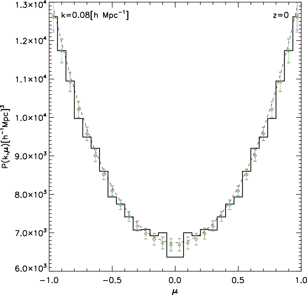
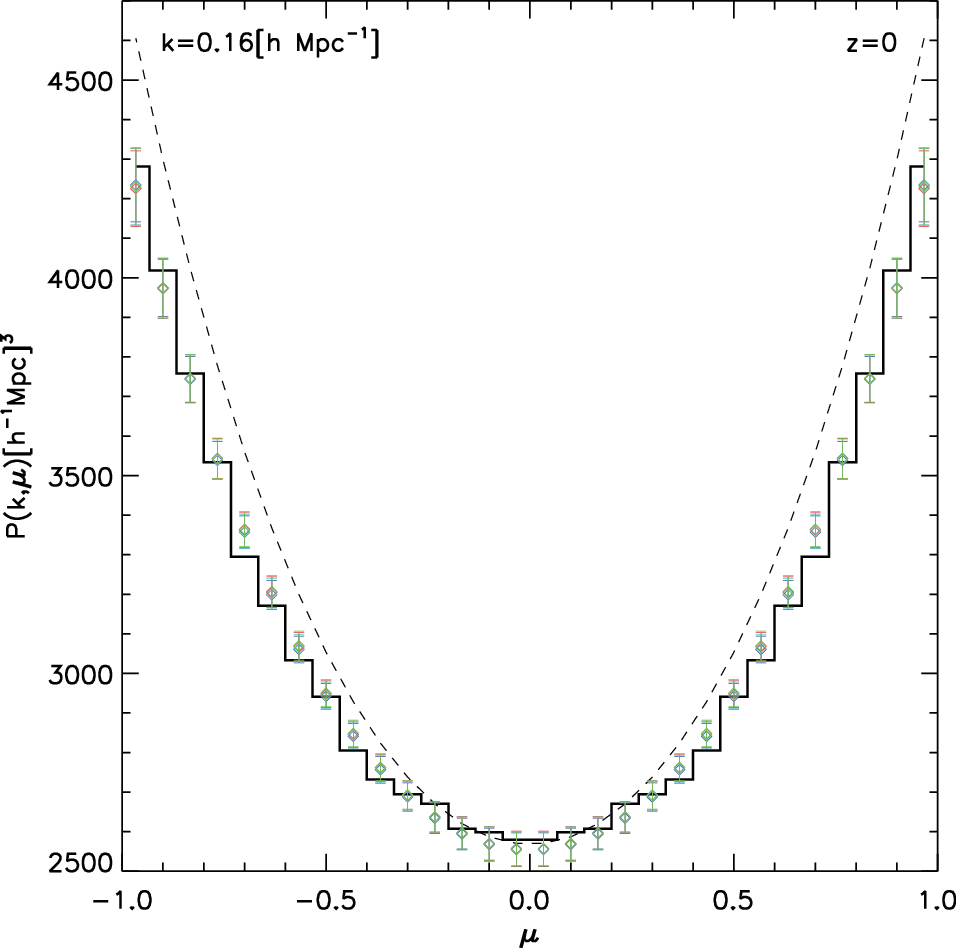
To have more insights on the results in Figs. 4 and 5, Fig. 6 show slices of the redshift-space power spectrum amplitudes, , as a function of the azimuthal angle , for a fixed radius : , and from the left to right panels, respectively. The histograms in each panel show the band powers measured from simulations, which are compared with the best-fit power spectra (different symbols) obtained in Fig. 4. The best-fit spectra are computed by inserting the best-fit parameters (band powers at each bins and the FoG parameters) into Eq. (11). As in Fig. 4, the different symbols are computed for the different FoG models. For comparison, we also plot the spectra, by dashed curves, which are computed by inserting the directly- measured , and in Eq. (11), without FoG term, i.e. . Hence, the difference between the dashed curve and the solid histogram clarifies how strongly the FoG affects the redshift-space power spectrum at each bin.
The two extreme cases are very distinctive. At small () the FoG effect is very small, and all the reconstructed power spectra can well match the input spectra independently of the FoG models. One the other hand, at the largest (), one can clearly see that the FoG effect is so strong that none of the Taylor () or Gaussian models (also or Lorentzian model) can fit the -dependence of redshift-space power spectrum. It is essential to add an additional parameter in the FoG model, like Taylor () model, to reproduce the simulation results. The middle panel shows the result at the intermediate scale (), where the FoG effect is mild and the FoG models of one parameter work to a good approximation.
Fig. 7 shows the posterior, marginalized distributions of the band powers, , , and at and the parameter of the Gaussian FoG model, which are obtained from the MCMC chains. Here we show the reconstruction results assuming the Gaussian FoG model, which well works at the scale of as shown in Fig. 6. The figure shows that, while the distribution of looks Gaussian, the distributions of , and show skewed, non-Gaussian distributions. In particular, the distribution of has a wide distribution and includes a region around , showing no constraint on the band power of . Given these results, we conclude that it is very difficult to reliably reconstruct based on the method developed in this paper, at least for a survey with survey volume Gpc3.
The origin of the skewed distributions in Fig. 7 is explored in Fig. 8, which shows the posterior distributions in a two-parameter sub-space between the parameters in Fig. 7. The figure clearly shows that the different parameters are correlated with each other after the nonlinear reconstruction. In particular, the parameter of Gaussian FoG model, shown here as an example, shows a strong correlation with the band power . Thus the band powers of different spectra () at different bins are correlated with each other, and the correlation needs to be properly taken into account for the power spectrum reconstruction.

Given such strong correlations between the band powers, how sensitive is the reconstruction of the power spectrum to a choice of the maximum wavenumber ? Fig. 9 studies this question. With increasing , the redshift-space power spectrum to use for the reconstruction is more affected by the FoG effect, and in turn the reconstructed and become increasingly affected by the FoG effect after marginalization. The figure shows the reconstructed and obtained when including the redshift-space power spectrum information up to and , respectively. For the triangle and square symbols, we assumed the Gaussian FoG model for comparison. The results for agree and are only slightly different at scales around , while the results for are systematically different. Since the Gaussian FoG model cannot well describe the FoG effect seen in simulations as implied in Fig. 4, the inaccuracy of the Gaussian FoG model causes a systematic underestimation in the band powers of if including the higher- modes. However, the two results for and agree over an overlapping range of , up to , within the error bars. For comparison, we also show the results obtained assuming and the Taylor () FoG model (see Eq. [14]). The Taylor () model is found to give a less biased reconstruction of , implying the importance of the assumed FoG model even around .
| FoG model | ||
|---|---|---|
| Gaussian () | ||
| Taylor () | ||
| Taylor () | (, ) | — |

Table 1 summarizes the best-fit FoG parameters and the marginalized confidence ranges that are obtained for the reconstructions at assuming different : and , respectively. For the Taylor () FoG model, the error of parameter is smaller than that of , because the parameter has a stronger dependence on as , than the -term does. Fig. 10 shows the 2D posterior distribution in the (,) sub-space.


| FoG model | ||
|---|---|---|
| Gaussian () | ||
| Taylor () | ||
| Taylor () | (, ) | — |
Nonlinearities in matter clustering are less significant at higher redshifts. Hence the likelihood reconstruction of power spectrum we are studying may work better for higher redshifts. Fig. 11 shows the results using simulations at , similarly to Figs. 4, 5, and 6. Note that we assumed as done in the reconstruction. In fact the FoG effect is smaller at than , e.g. as seen from the bottom-right panel of Fig. 11 compared to Fig. 6. However, the Taylor () FoG model seems still needed in order to better recover the simulation spectra. The bottom-right panel clearly shows that, although the FoG effect is smaller around compared to the result (Fig. 6), the Taylor () model better captures the simulation results around , showing a stronger dependence of than the Gaussian or Taylor () (or Lorentzian) models do. This implies that it is important to properly include the scale-dependent FoG effect for the power spectrum reconstruction, at least up to we have studied. As given in Table 2, a non-zero parameter is favored to capture the FoG effect seen in simulations. Fig. 12 shows the 2D posterior distribution in the (,) sub-space, displaying a strong correlation between the two parameters.

5.2 Reconstruction of halo power spectra
Now let us move on to the reconstruction of halo power spectra, which are more relevant for a galaxy survey, using the halo catalogs constructed from 70 simulation realizations (see § 4 for details). The halo clustering in redshift space is least affected by the FoG effect, because the halos are treated as points and the redshift distortion effect on halo clustering is caused only by their bulk motions in large-scale structure, not by the internal virial motion within one halo. Therefore we can naively expect a more accurate reconstruction of the density and velocity power spectra for halos based on the maximum likelihood method we have developed in this paper. However, unfortunately, this is not that simple as shown below.
For halo power spectrum we need to take into account the effect of shot noise arising from an imperfect sampling of the density fluctuation field due to the finite number of halos. In this case the maximum likelihood for power spectrum reconstruction needs to be modified as
| (18) | |||||
where is the shot noise contamination, and is the mean number density of halos. In the following we simply assume that the shot noise is not a free parameter and given by the mean number density of halos we use for the power spectrum reconstruction: (see Seljak et al., 2009, for a promising method to further suppress the shot noise contamination). The shot noise expression is not accurate for the actually measured power spectrum (Smith et al., 2007, e.g.), but the residual shot noise, even if exists, primarily contaminates to the spectrum that is proportional to , i.e. the density-density spectrum .
However the main obstacle we have faced is that we cannot reliably measure the velocity field of halos (see § 4.2.2 for details) and cannot therefore have the velocity-related power spectra, which are needed to assess the performance of our reconstruction method by comparing with the reconstructed spectra and . Rather we decided to use the dark matter (N-body particles) velocity field instead of estimating the halo velocity field, assuming that the halo bulk-velocity field is unbiased from the matter velocity field, which is often assumed in the literature.
Hence, before going to the halo spectrum reconstruction, we make a simple test to study whether or not the power spectrum reconstruction is affected by the shot noise contamination. This test can be done by applying our reconstruction method to the catalogs with reduced N-body particles. To be more precise we randomly select N-body particles from each simulation realization () until the number density of particles selected becomes the same to the density of halo catalogs, . Then by using the reduced N-body particles in each simulation we compute the redshift-space power spectrum taking into account redshift modulation due to the velocity field of each particle. These procedures preserve the underlying spectra of and . Thus we can compare the spectra with the spectra reconstructed by applying the maximum likelihood method to the redshift-space spectrum of reduced N-body particles, where the shot noise contamination is subtracted from the measured spectrum according to Eq. (18).
Fig. 13 shows the reconstruction results (symbols in each panels) for the catalogs of reduced N-body particles. The directly measured spectra in the left panel are similar to the curves in Fig. 4, although we found a small difference in the directly measured at due to the residual shot noise effect (Smith et al., 2007). Fig. 13 clearly shows that, even in the presence of shot noise, our reconstruction method recovers the power spectra to a similar precision to the results in Figs. 4, 5 and 6. Hence we conclude that the shot noise is not a serious source of systematics for our method.


Now we move to the reconstruction of halo power spectra. Fig 14 shows the results for halo catalogs at . First of all, the reconstruction can successfully recover the density power spectrum over a range of wavenumbers we consider, as a result of properly correcting for the shot noise and the redshift distortion. The accurate reconstruction of is relevant for the BAO experiments, and the results imply that our method may allow us to further use the broad-band shape of to improve cosmological constraints. However, in contrast to the results for N-body particles shown in Figs. 4 and 13, the reconstruction fails to recover the density-velocity power spectrum . The reconstructed for halos gives higher amplitudes than the directly measured power spectrum, irrespective of the different FoG models. In fact, as explicitly shown in the right panel, the measured redshift-space power spectrum shows greater amplitudes than predicted by the Kaiser formula (Eq. [11] with no FoG effect, i.e. ). The enhancement in the power spectrum amplitudes is opposite to the FoG effect, which always suppresses the amplitudes.
We argue below that the results in Fig. 14 can be understood by the nonlinearity effect on the redshift-space power spectrum. As we briefly discussed around Eq. (13), the nonlinear clustering causes a correction to the Kaiser formula of redshift-space power spectrum (also see Scoccimarro, 2004; Taruya et al., 2010, for a more extensive discussion). Assuming that the density perturbation is greater than the velocity field, which can be even more validated for highly biased halos with , the leading-order correction term is found to arise from the cross-bispectrum (see Eq. [13]):
| (19) |
We tried to measure this correction term from the simulations, but could not obtain the reliable results as the bispectrum measurement is very noisy. Instead we here use the perturbation theory prediction assuming a CDM cosmology (or equivalently Einstein gravity). In Appendix B we explicitly derive the leading-order correction term given as a function of the linear mass power spectrum. We find that the leading-order correction only contributes to the redshift-space power spectrum at the power of :
| (20) |
where is the correction term. Including the halo bias parameters, the correction term is expressed as
| (21) |
where ( is the growth rate) and and are the linear and nonlinear bias parameters. Note that we here assumed that the velocity field of halos is unbiased with respect to the velocity field of dark matter. Eq. (21) clearly shows that the nonlinearity correction term depends on halo bias parameters. The first term depends on the linear bias parameter as . Compared to the density-velocity power spectrum , which depends on as , the nonlinearity correction term can be more important for more biased halos, or equivalently more massive halos. Taruya et al. (2010) derived more comprehensive equations for dark matter including other nonlinear terms which arise from the cross-bispectra such as . The other terms are found to have the contributions of (), but depend on halo bias as . For highly biased halos with as halos we are studying, the term given by Eq. (21) has most dominant contribution. However, the perturbation theory is known to be less accurate for lower redshifts such as , due to the stronger nonlinear clustering effects. Hence the results shown here still need to be more carefully studied.
The dashed curves in the upper-left and -right panels of Fig. 14 show the results where we added the nonlinearity correction term to measured from the simulation assuming the Taylor FoG model: . To obtain the theory prediction of the nonlinearity correction term, we assumed and , where is estimated by comparing the density power spectra for dark matter and halos at small . More exactly we computed the correction power spectrum of using the full expression in Taruya et al. (2010), also taking into account the halo bias dependences on the different terms that are either proportional to or . Eq. (21) gives the similar shape, but about 10% higher amplitudes than the curves in Fig. 14. Interestingly, the nonlinearity correction term increases, rather than suppresses, the amplitudes of real-space power spectrum that is proportional to in the redshift-space power spectrum. The enhancement increases with increasing . We should also emphasize that such a nice agreement including the nonlinearity correction can be found only if using the Taylor-() FoG model. Given the fact that the redshift-space power spectrum of halos is least affected by the FoG effect, our results imply that the Taylor () model has more degrees of freedom than other one-parameter FoG models and can effectively capture higher-order contributions of () that arise from nonlinearity effects as studied in Taruya et al. (2010).
We also studied the halo power spectrum reconstruction using the halo catalogs constructed from simulations. We similarly found that the reconstructed power spectra of show greater amplitudes than expected from the measured . The nonlinearity correction term is found to similarly explain the reconstructed power spectrum, in slightly less agreement, if using the reconstructed power spectrum obtained from the Taylor FoG model. We have also found a subtle contamination of the residual shot noise for the results, and therefore we here show the results for for illustrative clarity.
To obtain more insights on the halo power spectrum results, in Fig. 15 we study the reconstruction results for using different halo catalogs where halos are selected with different mass thresholds. To be more precise, we made the new catalogs by employing higher mass threshold, (including more than 38 N-body member particles), rather than the threshold (20 particles) we have so far used. Note that the number density for more massive halos is , compared to for our fiducial halo catalogs. The estimated bias parameter is compared to . Fig. 15 shows the reconstruction power spectrum of for the different halo catalogs, compared to the density-velocity spectrum. The figure shows that the reconstructed spectrum for more massive halos has higher amplitudes than for less massive halos. The solid and dotted curves show the predictions obtained by adding the nonlinearity correction term (Eq. [21]) to the directly measured , where we used in the computation the linear bias parameters above and assumed for simplicity. The nonlinearity correction, which depends on the halo bias, fairly well reproduces the reconstruction results. In summary such nonlinearity correction terms need to be included when interpreting the reconstructed power spectra for halos, or more generally galaxies. We again emphasize that our method reconstructs band powers of the real-space power spectrum, which are proportional to in the redshift-space power spectrum, rather than the band powers of alone.
Finally we comment on the impact of nonlinearity correction on the reconstructions results for dark matter (N-body particles), which we showed in the preceding section. For the dark matter spectrum, which has by definition, the nonlinearity correction (Eq. [21]) is smaller compared to the results of halos. However, using the perturbation theory predictions, we found that the nonlinearity correction is not negligible. Including the nonlinearity correction improves agreement with the input power spectrum over a range of wavenumbers up to Mpc-1 for the Taylor-() FoG results shown in the middle panel of Fig. 5. However, the nonlinearity correction increases the disagreement at the larger . In summary we conclude that our reconstruction method can well recover the real-space power spectrum, which is proportional to in the redshift-space power spectrum, up to Mpc-1 for both dark matter and halos, if including the nonlinearity corrections.
6 Summary and Discussion
In this paper we have developed a maximum likelihood based method of reconstructing the real-space power spectra of density and velocity fields, from the two-dimensional, redshift-space clustering of dark matter and halos (supposedly galaxies). This method is developed in analogy with the CMB power spectrum reconstruction method (Verde et al., 2003).
By assuming the form of redshift-space power spectrum given by Eq. (16), we developed a method of reconstructing the band powers of and at each bins, being marginalized over uncertainties in the band powers at different bins and the parameters to model the FoG effect, in such a way that the likelihood of the redshift-space power spectrum measured becomes maximized. One assumption we have employed for the method is the functional form of redshift-space power spectrum (Eq. [16]), where the Kaiser formula and the FoG effect is given by multiplicative functions. In fact this form is expected based on the halo model picture (White, 2001; Seljak, 2001, also see Hikage et al. in preparation). The real-space power spectra, especially at such large length scales (), contains cleaner cosmological information in the linear or quasi-nonlinear regimes, and are relatively easier to develop a sufficiently accurate model by using a suit of simulations and/or refined perturbation theory. Furthermore, by measuring the velocity-related power spectra in a model-independent way, we can open up a new window of testing gravity on cosmological scales. That is, we can address whether or not the velocity field inferred is consistent with the gravity field inferred from the density field, because the density and velocity fields are related to each other via gravity theory.
We have carefully tested our method by comparing the reconstructed real-space power spectra with the spectra directly measured from simulations of 70 realizations, for dark matter (N-body particles) as well as halos. For matter power spectra (i.e. N-body particles), we showed our method nicely recovers the power spectra and over a range of scales and at redshifts and (see Figs. 4, 5 and 11), to accuracies within the statistical errors, if we use the Taylor () FoG model (see Eq. [14]), which has more degrees of freedom (2 parameters) than the other models, Gaussian, Lorentzian and single-parameter Taylor FoG models. Our results imply that the FoG effect seen in simulations has a complex scale-dependence, and is important to take into account the scale dependence in order to obtain an unbiased reconstruction of the band powers of and at scales down to . In other words, the FoG effect affects the redshift-space power spectrum over a wide range of wavenumbers. Hence an inaccurate modeling of the FoG effect causes a biased estimate of the power spectra. It is also worth noting that the reconstruction causes correlations between the band powers of different power spectra and at different -bins and the FoG model parameters (see Figs. 8 and 11).
For the halo power spectrum, we showed that our method again nicely recovers the density power spectrum over a wide range of wavelengths, up to (see Fig. 14). Such an accurate reconstruction of is very promising, because the shape and amplitude information of are sensitive to cosmological parameters such as the tilt and running index of the primordial power spectrum and neutrino masses (Takada et al., 2006; Saito et al., 2009; Saito et al., 2010, e.g.). On a measurement side, the halo power spectrum can be estimated from actual galaxy redshift survey, e.g. based on the method developed in Reid et al. (2010) where galaxy pairs with small spatial separations are clipped out. Although the halo power spectrum is supposed to be less contaminated by the FoG effect, it is very important to minimize the residual FoG contamination in order to extract unbiased cosmological information from the measured halo power spectrum. For example, since the FoG effect causes a suppression in the power spectrum amplitude, a residual FoG contamination would cause a bias in neutrino mass constraints because the main effect of massive neutrinos is also the suppression on power spectrum amplitude (Hikage et al. in preparation). Our method can give a robust way of measuring the density power spectrum, minimizing the FoG contamination.
For the halo velocity power spectrum , we found some difficulty. First of all, we could not reliably reconstruct the velocity field of halos from simulations, due to too sparse sampling of halos’ velocities. Hence we instead used the velocity field of dark matter (N-body particles) assuming that the large-scale bulk motions of halos are unbiased from the velocities of dark matter, which has been often assumed in the literature. Note that the real-space velocity field we considered here contains only the large-scale information at , and therefore is not affected by any virial motions within halos. As a result, we found that the reconstructed power spectrum of systematically differs from directly measured from the simulations (Fig. 14). In fact, the measured redshift-space halo power spectrum shows greater amplitudes than the spectrum inferred from the Kaiser formula of redshift-space spectrum, without the FoG effect that causes a suppression in the redshift-space power spectrum amplitudes.
Therefore we argued that the halo power spectrum is affected by the nonlinearity effect. In Appendix B, assuming a CDM cosmology or Einstein gravity, we derived the leading-order nonlinearity correction to the Kaiser formula of redshift-space power spectrum, which arises from the cross-bispectrum between the density and velocity perturbations. We meant by the leading-order term that the term appears to have the largest contribution, assuming that the density perturbation is greater than the velocity field at length scales of interest. We found that the leading-order contribution is proportional to and has greater amplitudes for more biased halos, i.e. more massive halos. We showed that adding the perturbation theory prediction to the simulation better matches the reconstructed power spectrum (see Fig. 14). We also found that, by using the different halo catalogs defined with different mass thresholds, the halo bias dependence of the nonlinearity correction is seen in the reconstructed power spectra of (see Fig. 15).
Hence a more appropriate statement for our maximum likelihood method is that the method can recover the real-space power spectra, which are proportional to and , respectively, in the measured redshift-space power spectrum, including marginalization over uncertainties in the FoG effect. In other words the reconstructed spectrum of is not necessarily the same as the density-velocity power spectrum , which we have used in our comparison. The nonlinearity effect on the real-space power spectrum of needs to be included if we want to use the reconstructed power spectrum to constrain cosmological parameters as well as to test gravity theory. On the other hand, we found that the power spectrum of is very noisy to reconstruct, for the ranges of wavenumbers and redshifts we have considered in this paper.
Recently Taruya et al. (2010) studied the redshift-space power spectrum including nonlinearity effects, based on the extended perturbation theory. They found that the nonlinear correction terms including the higher-order terms of have the contributions that are proportional to () in the redshift-space power spectrum. The comparison of the theoretical prediction with the reconstructed power spectrum based on our method is very interesting, and will be studied elsewhere.
One encouraging result is our method can unbiasedly recover the real-space density power spectrum even in the presence of redshift distortion effect. Given this result our method may offer even a new means of obtaining geometrical constraints on the Hubble expansion rate and the angular diameter distances beyond the usual BAO constraints. We have assumed throughout this paper that the underlying cosmology is known. However, this is obviously not true for an actual observation. In reality, we have to assume a reference cosmological model to perform the clustering analysis of galaxies, and the assumed cosmology generally differs from the underlying true cosmology. An imperfect cosmological model causes additional angular anisotropies in the measured redshift-space power spectrum – the so-called cosmological distortion. In terms of Eq. (16) an incorrect cosmology leads some power of the density power spectrum of to leak into the power spectrum with powers higher than in the redshift-space power spectrum. Contrary, if we seek the reconstructed of maximum amplitudes with varying reference cosmological models, we may be able to obtain the cosmological constraints (also see Padmanabhan & White, 2008, for a similar discussion). This method looks similar to the Alcock-Paczynski test (Alcock & Paczynski, 1979; Matsubara & Suto, 1996; Ballinger et al., 1996), but our method may have practical advantages: our method allows us to measure the real-space power spectrum of in a model-independent way as well as to derive cosmological constraints being marginalized over uncertainties in the FoG effect. The feasibility of this method is our future work and will be presented elsewhere.
Our reconstruction method is done in the two-dimensional Fourier space of . In practice one may want to exclude the Fourier modes around , which are more affected by the FoG effect. In our method it is straightforward to include a masking of the modes around ; that is, the real-space power spectra are reconstructed by using the Fourier modes in redshift space, excluding the modes around . We have tried several masking methods of , but could not find any significant differences from the results shown in this paper.
In this paper we have ignored some observational effects for simplicity. For example, to apply our method to actual data, we need to include effects such as survey window function and the curvature of the sky. These effects have been well studied (Tegmark et al., 2004, e.g.), and would be rather straightforward to include, although a further careful study needs to be done.
Acknowledgments
We thank E. Komatsu, B. Jain, T. Nishimichi, N. Padmanabhan, R. Sheth, D. Spergel and A. Taruya for useful discussion and valuable comments. This work is in part supported in part by JSPS Core-to-Core Program “International Research Network for Dark Energy”, by Grant-in-Aid for Scientific Research from the JSPS Promotion of Science, by Grant-in-Aid for Scientific Research on Priority Areas No. 467 “Probing the Dark Energy through an Extremely Wide & Deep Survey with Subaru Telescope”, by World Premier International Research Center Initiative (WPI Initiative), MEXT, Japan, and by the FIRST program “Subaru Measurements of Images and Redshifts (SuMRe)”.
References
- Albrecht et al. (2006) Albrecht A., et al., 2006, astro-ph/0609591
- Alcock & Paczynski (1979) Alcock C., Paczynski B., 1979, Nature, 281, 358
- Ballinger et al. (1996) Ballinger W. E., Peacock J. A., Heavens A. F., 1996, MNRAS, 282, 877
- Blake et al. (2011a) Blake C., et al., 2011a, ArXiv e-prints, arXiv:1105.2862
- Blake et al. (2011b) Blake C., et al., 2011b, ArXiv e-prints, arXiv:1104.2948
- Cole et al. (2005) Cole S., et al., 2005, MNRAS, 362, 505
- Crocce et al. (2006) Crocce M., Pueblas S., Scoccimarro R., 2006, MNRAS, 373, 369
- Dunkley et al. (2005) Dunkley J., Bucher M., Ferreira P. G., Moodley K., Skordis C., 2005, MNRAS, 356, 925
- Eisenstein et al. (2005) Eisenstein D. J., et al., 2005, ApJ, 633, 560
- Eisenstein et al. (1999) Eisenstein D. J., Hu W., Tegmark M., 1999, ApJ, 518, 2
- Fry & Gaztanaga (1994) Fry J. N., Gaztanaga E., 1994, ApJ, 425, 1
- Guzik et al. (2010) Guzik J., Jain B., Takada M., 2010, Phys. Rev. D, 81, 023503
- Guzzo et al. (2008) Guzzo L., et al., 2008, Nature, 451, 541
- Hamilton (1998) Hamilton A. J. S., 1998, in D. Hamilton ed., The Evolving Universe Vol. 231 of Astrophysics and Space Science Library, Linear Redshift Distortions: a Review. pp 185–+
- Jackson (1972) Jackson J. C., 1972, MNRAS, 156, 1P
- Jain & Bertschinger (1994) Jain B., Bertschinger E., 1994, ApJ, 431, 495
- Jain & Khoury (2010) Jain B., Khoury J., 2010, Annals of Physics, 325, 1479
- Jain & Zhang (2008) Jain B., Zhang P., 2008, Phys. Rev. D, 78, 063503
- Jennings et al. (2011) Jennings E., Baugh C. M., Pascoli S., 2011, MNRAS, 410, 2081
- Kaiser (1987) Kaiser N., 1987, MNRAS, 227, 1
- Lewis & Bridle (2002) Lewis A., Bridle S., 2002, Phys. Rev., D66, 103511
- Lewis et al. (2000) Lewis A., Challinor A., Lasenby A., 2000, ApJ, 538, 473
- Linder (2005) Linder E. V., 2005, Phys. Rev. D, 72, 043529
- Matsubara (2008a) Matsubara T., 2008a, Phys. Rev. D, 78, 083519
- Matsubara (2008b) Matsubara T., 2008b, Phys. Rev. D, 77, 063530
- Matsubara & Suto (1996) Matsubara T., Suto Y., 1996, ApJ, 470, L1+
- Padmanabhan & White (2008) Padmanabhan N., White M., 2008, Phys. Rev. D, 77, 123540
- Peacock (1999) Peacock J. A., 1999, Cosmological Physics
- Peacock et al. (2001) Peacock J. A., et al., 2001, Nature, 410, 169
- Peacock et al. (2006) Peacock J. A., Schneider P., Efstathiou G., Ellis J. R., Leibundgut B., Lilly S. J., Mellier Y., 2006, Technical report, ESA-ESO Working Group on ”Fundamental Cosmology”
- Percival (2005) Percival W. J., 2005, MNRAS, 356, 1168
- Percival & White (2009) Percival W. J., White M., 2009, MNRAS, 393, 297
- Pueblas & Scoccimarro (2009) Pueblas S., Scoccimarro R., 2009, Phys. Rev. D, 80, 043504
- Reid et al. (2010) Reid B. A., et al., 2010, MNRAS, 404, 60
- Reyes et al. (2010) Reyes R., Mandelbaum R., Seljak U., Baldauf T., Gunn J. E., Lombriser L., Smith R. E., 2010, Nature, 464, 256
- Saito et al. (2008) Saito S., Takada M., Taruya A., 2008, Physical Review Letters, 100, 191301
- Saito et al. (2009) Saito S., Takada M., Taruya A., 2009, Phys. Rev. D, 80, 083528
- Saito et al. (2010) Saito S., Takada M., Taruya A., 2010, ArXiv e-prints, arXiv:1006.4845
- Sasaki (1987) Sasaki M., 1987, MNRAS, 228, 653
- Schlegel et al. (2009) Schlegel D. J., et al., 2009, ArXiv e-prints, arXiv:0904.0468
- Scoccimarro (2004) Scoccimarro R., 2004, Phys. Rev. D, 70, 083007
- Seljak (2001) Seljak U., 2001, MNRAS, 325, 1359
- Seljak et al. (2009) Seljak U., Hamaus N., Desjacques V., 2009, Physical Review Letters, 103, 091303
- Shapiro et al. (2010) Shapiro C., Dodelson S., Hoyle B., Samushia L., Flaugher B., 2010, Phys. Rev. D, 82, 043520
- Simpson & Peacock (2010) Simpson F., Peacock J. A., 2010, Phys. Rev. D, 81, 043512
- Smith et al. (2007) Smith R. E., Scoccimarro R., Sheth R. K., 2007, Phys. Rev. D, 75, 063512
- Song (2010) Song Y., 2010, ArXiv e-prints, arXiv:1009.2753
- Song & Kayo (2010) Song Y., Kayo I., 2010, MNRAS, 407, 1123
- Song et al. (2011) Song Y., Sabiu C. G., Kayo I., Nichol R. C., 2011, JCAP, 5, 20
- Spergel et al. (2007) Spergel D. N., et al., 2007, ApJS, 170, 377
- Springel (2005) Springel V., 2005, MNRAS, 364, 1105
- Takada (2006) Takada M., 2006, Phys. Rev. D, 74, 043505
- Takada & Bridle (2007) Takada M., Bridle S., 2007, New Journal of Physics, 9, 446
- Takada et al. (2006) Takada M., Komatsu E., Futamase T., 2006, Phys. Rev. D, 73, 083520
- Takahashi et al. (2011) Takahashi R., Yoshida N., Takada M., Matsubara T., Sugiyama N., Kayo I., Nishimichi T., Saito S., Taruya A., 2011, ApJ, 726, 7
- Taruya et al. (2010) Taruya A., Nishimichi T., Saito S., 2010, Phys. Rev. D, 82, 063522
- Taruya et al. (2009) Taruya A., Nishimichi T., Saito S., Hiramatsu T., 2009, Phys. Rev. D, 80, 123503
- Tegmark et al. (2004) Tegmark M., et al., 2004, ApJ, 606, 702
- Verde et al. (2003) Verde L., et al., 2003, APJS, 148, 195
- Wang (2008) Wang Y., 2008, JCAP, 5, 21
- White (2001) White M., 2001, MNRAS, 321, 1
- White et al. (2010) White M., et al., 2010, ArXiv e-prints, arXiv:1010.4915
- White et al. (2009) White M., Song Y., Percival W. J., 2009, MNRAS, 397, 1348
- Yamamoto et al. (2010) Yamamoto K., Nakamura G., Hütsi G., Narikawa T., Sato T., 2010, Phys. Rev. D, 81, 103517
- Yamamoto et al. (2008) Yamamoto K., Sato T., Hütsi G., 2008, Progress of Theoretical Physics, 120, 609
- Zhang et al. (2008) Zhang P., Feldman H. A., Juszkiewicz R., Stebbins A., 2008, MNRAS, 388, 884
- Zhang et al. (2007) Zhang P., Liguori M., Bean R., Dodelson S., 2007, Physical Review Letters, 99, 141302
Appendix A Likelihood function of redshift-space power spectrum
In this appendix we derive the likelihood function of redshift-space power spectrum. To do this, we assume that the density fluctuation field of large-scale structure tracers (matter or galaxies) is Gaussian and obeys the following Gaussian likelihood function:
| (22) |
where is the density fluctuation field (of matter or galaxies), is the correlation matrix between the fields and , is the inverse matrix, and is the determinant of the matrix . The covariance matrix or the correlation function, , can be expressed in terms of the power spectrum as
| (23) | |||||
where is the survey volume. Given a finite-volume survey, we introduced the discrete Fourier transformation of the density field (Takada & Bridle, 2007, e.g. see), where the fundamental Fourier mode is given by the survey size; (). Here we ignored survey geometry and boundary effects for simplicity. Therefore the inverse of the covariance matrix can be given as
| (24) |
This can be proved because the product of the covariance matrix and its inverse matrix satisfies the orthogonal relation, which is formally computed as
| (25) | |||||
where is the Kronecker-type delta function; if within the bin width, otherwise (see Takada & Bridle (2007)).
Using the equations above, the argument in the exponential of Eq. (22) can be reduced to the following form in Fourier space:
| (26) | |||||
Note that, in equation above, I assumed that and have same dimensions such that the combination becomes dimension-less.
Therefore the log-likelihood function of density fluctuation field (Eq. [22]) is reduced to the log-likelihood function of the power spectrum:
| (27) |
where we have ignored the constant additive term. The log-likelihood above is rewritten in terms of the power spectrum estimator as
| (28) |
Here is the power spectrum estimator
| (29) |
where the summation is over Fourier modes satisfying the condition that the wavevector lies in the bin labeled by the length and the azimuthal angle between the line-of-sight direction and the wavevector, , and is the number of independent Fourier modes: for . The -dependence of power spectrum accounts for redshift distortion effect.
Adding the constant term into the equation above such that the log-likelihood function can be maximized if the theory power spectrum is equal to the estimated one, we can arrive, as in the CMB case (Verde et al., 2003), at the expression:
| (30) |
Hence we can use this log-likelihood to estimate the underlying power spectrum at each bin, given the observed power spectrum .
Appendix B Nonlinear correction terms of the Kaiser formula
In this appendix, following the method developed in Scoccimarro (2004) and Taruya et al. (2010), we derive the leading-order correction term of higher-order perturbations to the Kaiser formula for the redshift-space power spectrum, assuming a CDM cosmological model based on the Einstein gravity.
Let us begin our discussion with recalling that the redshift distortion effect on a given tracer of the large-scale structure is recognized as a mapping between redshift- and real-space positional vectors:
| (31) |
where and are the positional vectors in redshift- and real-spaces, respectively, is the line-of-sight component of the normalized peculiar velocity (see around Eq. [8]) and is the unit vector of the line-of-side direction in the real-space coordinate system. The mass or number conservation law gives the relation between the density perturbations in redshift- and real-spaces:
| (32) |
Therefore the Fourier transform of the redshift-space density perturbation can be expressed in terms of the real-space density and velocity perturbation fields as
where we have expressed the peculiar velocity field as the velocity-divergence field as (see around Eq. [10]), and . On the third equality on the r.h.s. of the equation above, we have used the Jacobian, to make the integration variable change, . Here, given the fact that the density perturbation is greater than the velocity perturbation, we kept the leading-order nonlinear correction term which has the order of and ignored the higher-order terms than .
Therefore, the nonlinear correction term to the redshift-space power spectrum is found to be
| (34) |
where the bispectrum is defined as
| (35) |
Using the perturbation theory of structure formation (Jain & Bertschinger, 1994, e.g.) we can express the bispectrum in terms of the linear power spectrum as
where , at the linear order for our notation and the kernels and are defined as
For halo clustering, we need to further take into account halo bias. Here we simply assume that halo bias is deterministically given as a function of the underlying mass density field (Fry & Gaztanaga, 1994, e.g.):
| (38) |
where and are the linear and nonlinear bias parameters. On the other hand we assume that the velocity field of halos is unbiased to the velocity field of dark matter. Then we can similarly compute the correction term to the redshift-space power spectrum of halos:
| (39) | |||||
We can further simplify the equation (39) by using the usual formula developed in Appendix A and B of Taruya et al. (2010) (also see Matsubara (2008b)). The formula tells that the following equation holds for an arbitrary scalar function :
| (40) |
where and
| (41) |
Here we have introduced the integration variable transformations as and .
Therefore, by comparing Eqs. (39) and (40), we can find that the nonlinear correction term to the Kaiser formula of the redshift-space power spectrum is proportional to . That is, the leading-order nonlinear correction term only contaminates to the density-velocity power spectrum in the Kaiser formula. If we define the correction term as , we find that the real-space power spectrum is given as
| (42) |
Eq. (42) has several interesting implications. First of all, the nonlinear correction term scale with halo bias as . Since the density-velocity power spectrum for halos scales as , the correction term can be more important for more biased halos. Secondly, once the gravity theory is assumed (here the Einstein gravity), the correction term can be computed as a function of cosmological models. Taruya et al. (2010) further derived other correction terms arising from the higher-order perturbations than , and then showed that the nonlinear correction term can show remarkable nice agreement with the simulation results. In the main text (see Sec. 5.2) we use Eq. (42) to explain the power spectrum reconstruction results for halos, where we found that the reconstructed power spectrum, which is proportional to , shows sizable difference from the input .